Stereo-Event-Camera-Technique for Insect Monitoring

Regina Pohle-Fr

ohlich

, Colin Gebler and Tobias Bolten

Institute for Pattern Recognition, Niederrhein University of Applied Sciences, Krefeld, Germany

Keywords:

Event Camera, Segmentation, Insect Monitoring, Depth Estimation.

Abstract:

To investigate the causes of declining insect populations, a monitoring system is needed that automatically

records insect activity and additional environmental factors over an extended period of time. For this reason,

we use a sensor-based method with two event cameras. In this paper, we describe the system, the view volume

that can be recorded with it, and a database used for insect detection. We also present the individual steps

of our developed processing pipeline for insect monitoring. For the extraction of insect trajectories, a U-Net

based segmentation was tested. For this purpose, the events within a time period of 50 ms were transformed

into a frame representation using four different encoding types. The tested histogram encoding achieved the

best results with an F1 score for insect segmentation of 0.897 and 0.967 for plant movement and noise parts.

The detected trajectories were then transformed into a 4D representation, including depth, and visualized.

1 INTRODUCTION

Climate and human-induced landscape changes have

a major impact on biodiversity. One process that has

been observed and scientiﬁcally documented in recent

years is the decline of many insect species (Hallmann

et al., 2017). To better understand the causes, biodi-

versity monitoring at the species level is needed, but is

currently hampered by several barriers (W

agele et al.,

2022). For example, automated species identiﬁca-

tion is difﬁcult because only a limited number of test

datasets for AI-based techniques for the various mon-

itoring methods are currently available (Pellegrino

et al., 2022). On the other hand, manual monitoring of

insects is costly, which means that often only small ar-

eas and limited time periods are surveyed. Due to the

high cost, such monitoring is only done on a random

basis, so that comparisons for the same habitat type

between regions or between different time periods are

not possible. In addition, manual observations may be

subject to unintentional bias (Dennis et al., 2006) and

their quality may depend on the expertise of the ob-

server (Sutherland et al., 2015). Furthermore, because

the observational sources in this case e.g. as images

of the measurements are not preserved, the accuracy

of the data may be questioned later. This is especially

true because human attention is low for non-foveal

https://orcid.org/0000-0002-4655-6851

https://orcid.org/0000-0001-5504-8472

visual tasks and for moving objects (Ratnayake et al.,

2021).

Another problem is that even many automated

methods (traps, camera-based systems) can only sur-

vey very small areas. The data thus obtained are

not easily extrapolated to larger areas. In addition,

species interactions or changes within populations are

often difﬁcult to detect due to the limited time win-

dow considered or the size of the observation patch.

Suitable technologies for large-scale and long-term

automated biodiversity monitoring are still lacking

agele et al., 2022).

For this reason, we want to develop a new mon-

itoring method using event cameras. The operation

and output paradigm of this sensor is fundamentally

different from conventional cameras. For example,

the event camera does not capture images at a ﬁxed

sampling rate, but generates event streams (Gallego

et al., 2020). For each detected brightness change

at a pixel position above a deﬁned threshold, the x-

and y-coordinate, a very precise time stamp t in mi-

croseconds and an indicator p for the direction of the

brightness change are recorded. Other advantages

compared to conventional CCD/CMOS sensors in-

clude higher dynamic range, lower power consump-

tion, smaller data volume, and much higher temporal

resolution. Since each pixel of an event camera oper-

ate independently and asynchronously based on rela-

tive brightness changes in the scene, they can also be

used under difﬁcult lighting conditions (strong bright-

Pohle-Fröhlich, R., Gebler, C. and Bolten, T.

Stereo-Event-Camera-Technique for Insect Monitoring.

DOI: 10.5220/0012326500003660

Paper published under CC license (CC BY-NC-ND 4.0)

In Proceedings of the 19th International Joint Conference on Computer Vision, Imaging and Computer Graphics Theory and Applications (VISIGRAPP 2024) - Volume 3: VISAPP, pages

375-384

ISBN: 978-989-758-679-8; ISSN: 2184-4321

375

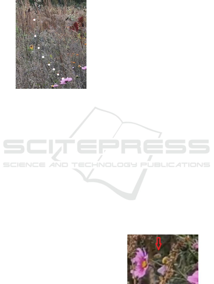
Figure 1: Position of a bee (white dots) during takeoff in

eight frames captured at 30 frames per second.

ness differences in the scene). First tests with this sen-

sor for insect monitoring have already been success-

fully performed (Pohle-Fr

ohlich and Bolten, 2023).

In this paper we want to discuss further develop-

ments of this approach. These major contributions are

• the use of a stereo event camera setup, so that 4D

data points (x, y, z, t) can be recorded

• the investigation of different event encoding types

for trajectory extraction

• the description of the depth calculation pipeline.

The rest of this paper is structured as follows. Sec-

tion 2 gives an overview of related work. Section 3

describes the dataset acquisition setup. In Section 4,

the currently used processing pipeline is explained

and in Section 5, the obtained results are presented

and discussed. Finally, a short summary and an out-

look on future work is given.

2 RELATED WORK

The use of AI methods has signiﬁcantly improved in-

sect monitoring in recent years. Although the use of

traps is still a common method for determining the

biomass and abundance of individual insect species,

whereas in the past traps were mostly evaluated by

humans, this is now being done in part with the

help of DNA metabarcoding (Pellegrino et al., 2022)

or automated camera systems. The cameras cap-

ture single images of speciﬁc locations where insects

are attracted by targeted lighting, colored stickers,

or pheromones in order to identify and count them

((Qing et al., 2020), (Marcasan et al., 2022), (Dong

et al., 2022)). During image acquisition, the insects

hardly move and can be well segmented due to the

uniform background color used at these locations.

To detect interactions between different insect

species, video cameras are usually used to examine

small areas with very few plants. Under these condi-

tions, good detection results can be obtained for some

insects, such as bees ((Bjerge et al., 2022), (Droissart

et al., 2021)). However, problems arise with trajec-

tory detection (Figure 1), since required high tem-

poral resolution cannot be used due to the required

storage space. In addition, image compression (Fig-

ure 2) is required for long-term monitoring for the

same reason, which makes insect detection difﬁcult

and error-prone.

The monitoring method proposed in this paper

uses event cameras. Various approaches for segmen-

tation and classiﬁcation of event data can be found

in the literature (Gallego et al., 2020). A common

method for data analysis is to convert the event stream

into 2D images. In this process, all events within

a time window of ﬁxed length or a ﬁxed number of

events are projected into an image using different en-

coding methods preserving different amounts of tem-

poral information (e.g., binary encoding, linear time-

surface encoding, polarity encoding). Then, different

neural networks (e.g., U-Net, Mask-RCNN) are used

for segmentation. In addition, neural networks that

take a point cloud as input (PointNet++, LSA-Net, A-

CNN) are used for both segmentation and classiﬁca-

tion ((Bolten et al., 2022a), (Bolten et al., 2023b)).

3 DATASET RECORDING SETUP

3.1 Used Sensor System

Contrary to the work of (Bolten et al., 2023b) on hu-

man activity recognition, the motion of insects does

not take place on planes, but in 3D space. For this

reason, capturing the scene with only one camera to

estimate the z-coordinate as in (Bolten et al., 2022b)

Figure 2: Poor visibility of a honeybee (see arrow) due to

H.264 video compression.

VISAPP 2024 - 19th International Conference on Computer Vision Theory and Applications

376

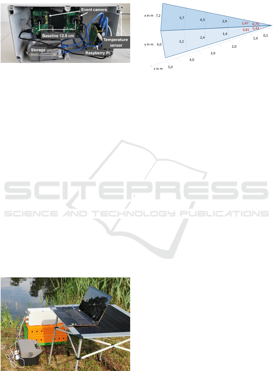
Figure 3: Stereo system with two event cameras.

is not sufﬁcient. Therefore, a stereo system was cho-

sen for image acquisition. By capturing the depth

information, it is also possible to make assumptions

about the insect’s size and ﬂight speed and use them

to group the insects. Figure 3 shows the setup of our

measurement system.

Two parallel event camera IMX636 HD sensors

distributed by Prophesee (Prophesee, 2023b) with an

image resolution of 1280 x 720 pixels, each equipped

with an 5mm wide-angle lens, are synchronized in

time and connected to a RaspberryPi 4B running the

data acquisition software. The event stream gener-

ated by each camera is written to an external hard

drive. Additionally, a temperature sensor is integrated

into the measurement setup. The camera system is

recharged by a solar panel if required, to enable mea-

surements in any terrain. Figure 4 shows our mea-

surement system in action. For manual logging and

labeling of insect activity, an additional event camera

was connected to a laptop in order to display the ref-

erence data.

3.2 Covered View Volume

In order to obtain information about the detection

range of our monitoring system, it was ﬁrst deter-

mined by calculation. Subsequently, the theoretically

Figure 4: System in action.

Figure 5: View volume.

calculated values were evaluated by throwing refer-

ence objects similar in size to certain groups of in-

sects at a deﬁned distance into the ﬁeld of view of the

camera system. The measured values conﬁrmed our

calculations. Figure 5 shows the obtained view vol-

ume. The black numbers show the calculated values

and the red numbers show the experimentally deter-

mined values.

Insects with a size of 5 x 2 mm², which is approxi-

mately the size of a mosquito, can be reliably detected

up to a distance of 2 m from the camera. The area

over which these insects can be reliably recognized

is 2.9 m² considered in the top view. Insects with a

size of 10 x 5 mm², which corresponds to the size of

a house ﬂy, can be reliably identiﬁed up to a distance

of 5 m from the camera. These insects can be located

on an covered ground area of 18 m². Insects with a

size of 15 x 10 mm², which corresponds to the size

of a honey bee, can still be reliably recognized at a

distance of 7 m from the camera. In this case, the

covered ground area is 35 m². This is a signiﬁcant in-

crease compared to the ground area of 1 m² used in

manual insect counting.

3.3 Used Database

For the detection of insect ﬂight paths, on the one

hand, the labeled dataset from (Pohle-Fr

ohlich and

Bolten, 2023) was used, which was, however, only

recorded with one camera and not as stereo data. On

the other hand, additional monocular event data were

recorded and labeled. These recordings were taken in

the evening in a garden with grass, and in the morning

and in the afternoon on a balcony with ﬂowers in bal-

cony boxes. Because of the different scenarios, plant

movement and other environmental factors varied.

All ﬁles were labeled to include two classes: In-

sect trajectory events and events due to noise and

plant movements. Figure 6 shows a section of one

of the labeled datasets, with the insect class events

colored red and the environment class events colored

white. Thus, eight recordings with a total dataset

Stereo-Event-Camera-Technique for Insect Monitoring

377

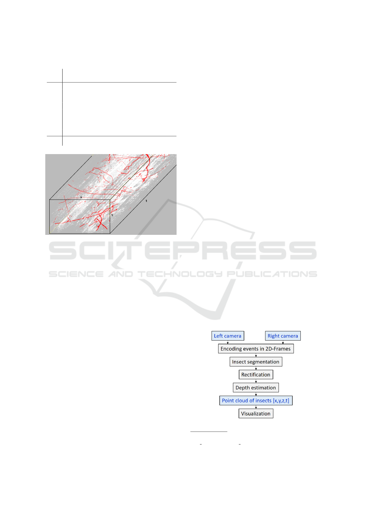
Table 1: Structure of the dataset.

No. Content Size No. of No. of

in sec insect events other events

1 Meadow 30.94 834 373 1 109 131

2 Garden 100.01 1 054 489 200 102

3 Garden 97.40 1 022 401 137 577

4 Garden 156.58 935 939 545 659

5 Balcony 73.24 1 407 740 656 936

6 Balcony 61.12 160 504 756 339

7 Balcony 16.10 78 832 1 037 434

8 Balcony 78.85 1 407 740 656 936

614.24 6 902 018 5 100 114

Figure 6: Example of the labeled insect dataset No. 1

(Events from ﬂight paths are red and events from environ-

mental effects are colored white.).

length of 10 minutes and 14 seconds were available

for neural network training. The basic properties of

the dataset are shown in Table 1. It can be seen that

the plant events are currently still slightly underrepre-

sented.

4 FLIGHT PATH

SEGMENTATION

4.1 Software Pipeline

The 4D trajectory determination for the individual in-

sects is realized in several steps. After recording the

event streams with the two cameras, they are ﬁrst en-

coded into 2D frames for segmentation with a CNN.

The events classiﬁed as insects are then transformed

into rectiﬁed coordinates before the depth is calcu-

lated from the disparity of the pixels in each of two

corresponding projected views from the left and right

camera. Finally, the 4D points available after this step

are visualized. The process is illustrated in Figure 7.

The individual steps are described in more detail be-

low.

4.2 Event Encoding

There are a variety of methods for encoding and pro-

cessing the output stream of an event camera (Gal-

lego et al., 2020). Often, the events are converted into

classical 2D images and then processed using estab-

lished image processing methods. This approach was

also chosen for the insect data. Direct processing as

a point cloud would require a reduction in the num-

ber of events by applying downsampling methods.

However, since the insect trajectories represent very

ﬁne structures within the point cloud, these would be

lost. Splitting the output data into different window

regions, as in (Bolten et al., 2023a), would also be

problematic because insects move very fast and thus

ﬂy over several windows in a very short time. The

data would then have to be reassembled for ﬁnal anal-

ysis. Since time information is lost when event data is

projected into a 2D binary or polarity representation,

various encoding methods have been described in the

literature to preserve this information. Four different

encoding approaches have been investigated for de-

tection of ﬂight trajectories.

• Histogram Encoding

A simple way of encoding is to create a his-

togram. For a given time window, the number of

events per pixel position is determined separately

for each polarity, with the maximum number set

to 5 (Prophesee, 2023a)

. This results in a two-

channel encoding. Fast moving objects, such as

insects, have lower frequencies compared to slow

and cyclically moving objects, such as plants. In

the experiments performed, we used a time win-

dow of 50 ms for event accumulation.

• Linear Timesurface Encoding

The linear time surface is another method of en-

coding the time information of events in a 2D rep-

Figure 7: Software pipeline for detection of ﬂight paths.

https://docs.prophesee.ai/stable/tutorials/ml/

data processing/event preprocessing.html

VISAPP 2024 - 19th International Conference on Computer Vision Theory and Applications

378

resentation. In this method, the scaled time stamp

of the last event that occurred is stored in each

pixel, again considering the polarities separately.

This yields to a two-channel encoding. The scal-

ing is linear in the range between 0 and 255. In our

experiments we used a time window of 50 ms.

• Event Cube Encoding

Event cubes were developed to combine the infor-

mation from the histogram with the time informa-

tion from the linear timesurface. In event cubes,

each time bin is further divided into three micro

time bins. Instead of counting an event based on

its position and time stamp as in the histogram, the

event is counted linearly weighted according to its

time distance from the center of the neighboring

micro time bins (Prophesee, 2023a)

. Since the

summation is done separately for each polarity.

This results in a six-channel encoding and leading

to a higher computational complexity for training

and inference of neural networks compared to the

other encodings. To obtain enough events in a

frame for the calculation, a time window of 50 ms

was used.

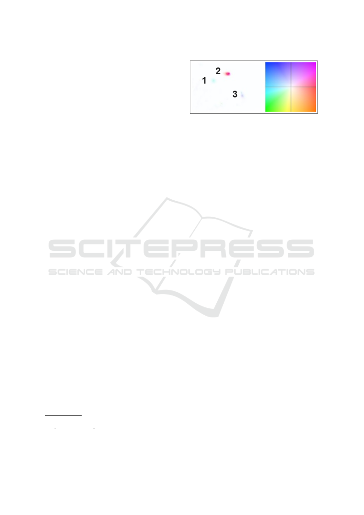
• Optical Flow Encoding

Finally, to encode the temporal information con-

tained in the event stream, the optical ﬂow was

also examined, since insects usually move very

fast and in arbitrary directions, while plants move-

ments are slower and occur only in certain direc-

tions.

There are several ways to estimate optical ﬂow.

The algorithm provided in the Metavision SDK

for computing sparse optical ﬂow has the disad-

vantage that clustering is performed beforehand

(Prophesee, 2023a)

. Experiments have shown

that, for insect movements in the background with

very few points in the projected image plane, no

optical ﬂow value is calculated.

For this reason, the dense optical ﬂow algorithm

provided by the Metavision SDK was used as

well. Since the data from the insect crossings con-

tains very few objects within a short time window,

training the neural network used for the dense

ﬂow calculation did not produce satisfactory re-

sults, so we used a pre-trained network with the

weights provided in the SDK for our calculations.

As with the other methods, the time window for

optical ﬂow calculation was 50 ms. From the two

predicted components of the ﬂow vector, we have

https://docs.prophesee.ai/stable/tutorials/ml/

data processing/event preprocessing.html

https://docs.prophesee.ai/stable/samples/modules/cv/

sparse ﬂow cpp.html

Figure 8: Example for optical ﬂow prediction for three dif-

ferent moving objects. The adjacent color wheel was used

for display. The intensity indicates the magnitude of the

ﬂow and the color the direction of the movement.

calculated the magnitude from this estimated ve-

locity vector and direction as the angle to x-axis

between 0 and 360 degrees. Again, resulting in

a two-component encoding. It should be noted,

however, that the computational cost of determin-

ing the optical ﬂow is high. An example of the

predicted optical ﬂow can be found in Figure 8.

In our current investigations, all events in our dataset

were encoded using the four encoding methods, re-

sulting in a total number of 12230 images of each en-

coding.

4.3 Insect Segmentation

After frame encoding, classical 2D networks can be

used for semantic segmentation of trajectories. A

typical network that can perform segmentation with

a relatively small amount of input data is the U-Net

(Ronneberger et al., 2015). It is an encoder-decoder

network with a typical symmetric structure. The en-

coder part is used for feature extraction, where the

convolutional and pooling layers also lead to down-

sampling and information concentration, but also to

spatial mapping reduction. Upsampling is then per-

formed in the decoder section to restore the original

size of the image and achieve high resolution segmen-

tation at the pixel level. Upsampling layers are used

here. In addition, there are skip connections between

the encoder and decoder to integrate the features of

the different layers of the encoder into the decoder.

The U-Net is a very lightweight network that has

already been used to segment trajectories in (Pohle-

ohlich and Bolten, 2023). For the segmentation

with the U-Net, we used a network depth of four lay-

ers in combination with a loss function weighted by

the class frequency of the individual pixels.

4.4 Camera Calibration

To facilitate stereo vision, the camera heads must

ﬁrst be calibrated. This serves the purposes of ﬁrstly

Stereo-Event-Camera-Technique for Insect Monitoring

379

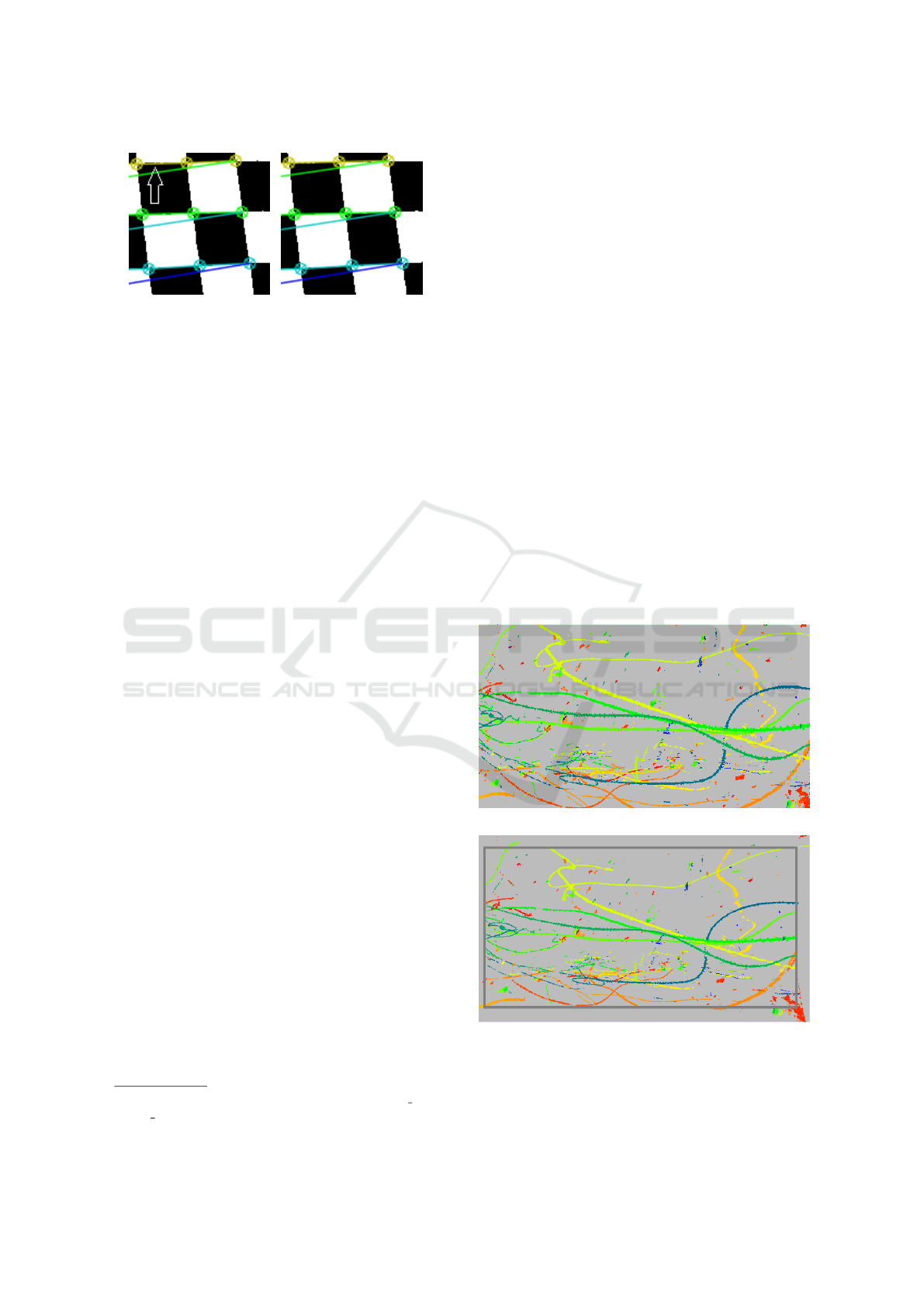
(a) Points found in a single

detection.

(b) Average of multiple de-

tections.

Figure 9: Comparison of a single detection and averaged

object points.

undistorting the pixel coordinates, causing distances

between pixels to be unaffected by their positions in

the pixel array, and secondly determining the cam-

eras’ exact position relative to one another. This al-

lows us to align the event streams spatially and sim-

plify the matching of corresponding events later.

Typically, calibration is performed by detecting

readily discernible points of an object with a known

shape and determining the transformation matrices

matching these points’ detected pixel coordinates

with the presumed object point coordinates. For

stereo calibration, a transformation is computed that

maps the coordinate system of one camera to that of

the other in addition to the undistortion transforma-

tion.

Commonly, a chessboard pattern is used as the

known object, detecting the inside corners between

squares. For a frame camera, this can be a physical

chessboard of which photos are taken at various an-

gles and relative positions. Calibrating an event cam-

era introduces the complication that events are only

generated where there are changes in the scene. This

results in a static chessboard not being captured by

the camera. Moving a chessboard around in front

of the camera would introduce motion and make it

hard to acquire exactly corresponding object points.

To record a pattern with an event camera without

movement, it must change in brightness. One way to

achieve this is by displaying the calibration pattern on

a screen and making it ﬂash. We displayed a ﬂashing

black and white chessboard on a white background on

an IPS screen, causing events to be generated by the

black squares. The dimensions of the squares were

2.2 cm × 2.2 cm. We use the Metavision SDK im-

plementation (Prophesee, 2023a)

to detect the inside

corners in frames generated from 10 ms of events. To

mitigate inaccuracies in corner localization, we take

several static recordings of the chessboard from mul-

https://docs.prophesee.ai/stable/api/python/core ml/

corner detection.html

tiple angles and average the point positions of all de-

tections for each individual recording. The result of

this approach is illustrated in Figure 9.

Once the object points are acquired, intrinsic and

extrinsic camera parameters are calculated the same

way as they would be for a frame based camera. We

use the functionality provided by the Metavision SDK

to calculate each camera’s intrinsic parameters and

use OpenCV (Bradski, 2000) library functions to ac-

quire the extrinsic parameters based on the previously

acquired object points.

4.5 Depth Value Computation

The ﬁrst step in the depth calculation after the cam-

era calibration is the rectiﬁcation of the images to en-

sure that by reducing the correspondence problem by

the epipolar condition, the search for corresponding

points only has to be done along one image row. The

result is shown in Figure 10 for a part of the dataset.

The rectiﬁcation is followed by a search for cor-

responding point pairs. For this purpose, the events

detected as insects in the two camera streams are pro-

jected into an image over a longer time period of em-

pirically determined 250 ms each, where the value at

the pixel position corresponds to the time stamp (see

(a) Plain display.

(b) Data after rectiﬁcation.

Figure 10: Part of a dataset before and after the rectiﬁca-

tion step (the frame indicates the undistorted section, and

the colors of the individual events correspond to the time

stamp).

VISAPP 2024 - 19th International Conference on Computer Vision Theory and Applications

380

(a) Image of the left camera.

(b) Image of the right camera.

Figure 11: Left and right images and detected correspond-

ing points.

Figure 11). The differences in the trajectories seen

in the ﬁgure between the left and right camera images

may be due to either differences in occlusion during

perspective projection from different viewing angles,

or differences in segmentation.

To determine depth, for each pixel in the right im-

age, a corresponding pixel in the left image is located,

including not only the same row but also two rows be-

low and above to account for calibration inaccuracies.

A pixel is considered corresponding if the time dif-

ference is minimal and less than 1.5 ms. This thresh-

old is empirically determined and compensates for in-

accuracies during synchronization. The difference of

the x-coordinate between the determined correspond-

ing values is stored as a disparity value. In the last

step, the 4D world coordinates (x, y, z, t) are calcu-

lated from these disparities and the reprojection ma-

trix determined during camera calibration, where the

coordinates are relative to the optical center of the left

camera.

5 RESULTS

To evaluate the different encoding methods with re-

spect to the quality of the segmentation, the dataset

described in Section 3.3 was used, which, however,

does not contain any stereo data. To evaluate the qual-

ity of the depth estimation, two additional datasets

were used. However, no segmentation ground truth

was available.

5.1 Segmentation Results

To investigate the segmentation quality, our dataset

of 12230 images was partitioned using 3690 images

as a test set. To ensure that the network had not

already seen immediately adjacent images, the total

number was ﬁrst divided into blocks of 10 images

each, from which 369 blocks (30%) were randomly

selected. Each block contained a time interval of half

a second. Due to the fast movement of the insects, this

ensured sufﬁcient variability between training and test

sets.

To compare segmentation results the F1 score was

used. The best results were obtained with histogram

encoding after 100 training epochs. The individual

results are shown in Table 2. The F1 scores for the

BACKGROUND class representing pixels in the en-

coding without any triggered events were 0.999 in all

cases and are therefore not included in the table.

When looking at the result images, it became clear

that the two classes of interest were mostly segmented

slightly too large, resulting in a low F1 value. There-

fore, only those class predictions where events ac-

tually occurred were considered in a post-processing

step. This makes sense because only these are impor-

tant for propagating the results back to the original

3D event stream for depth estimation (Pohle-Fr

ohlich

and Bolten, 2023). The results of this post-processing

are given in Table 2b. The F1 values improved for all

classes and encodings. Again, the best results were

obtained for the histogram encoding.

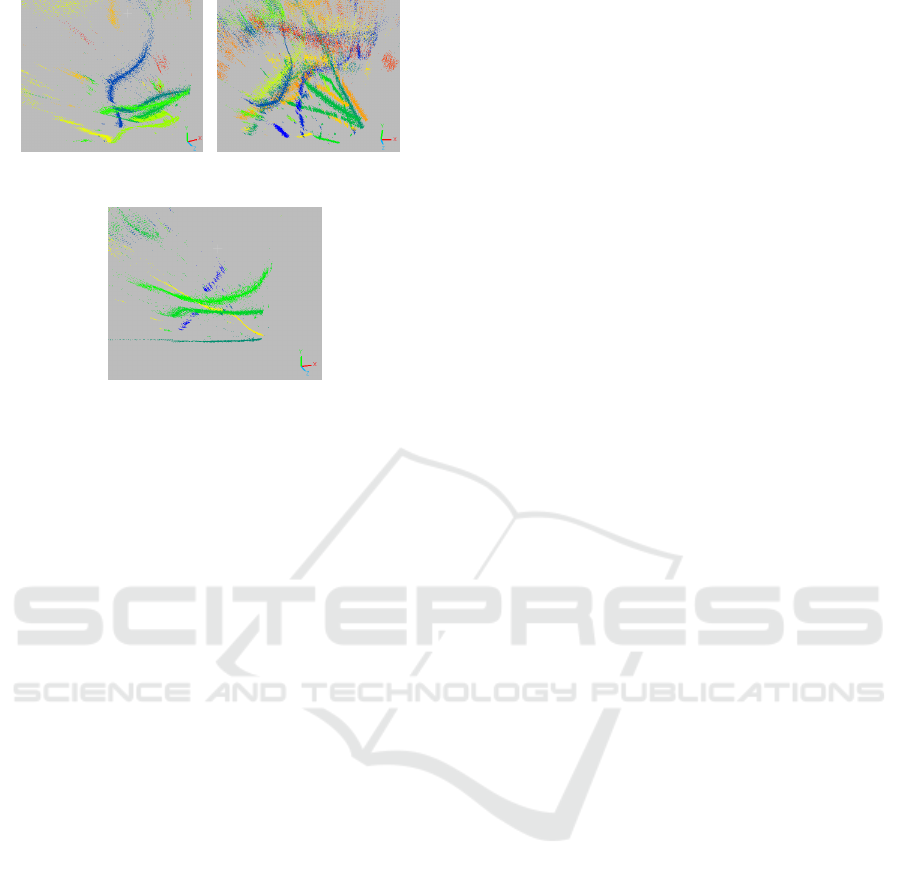
Using the trained weights to predict events asso-

ciated with insect ﬂight paths yields to similar re-

sults for two datasets taken from different views of

a meadow (Figure 13b) that were not included in the

training set. Figure 12 shows a section of the point

cloud visualizing all events for three of the used en-

coding methods. All points detected by event cube

encoding are colored red, all detected by optical ﬂow

encoding are colored green, and all detected by his-

Stereo-Event-Camera-Technique for Insect Monitoring

381

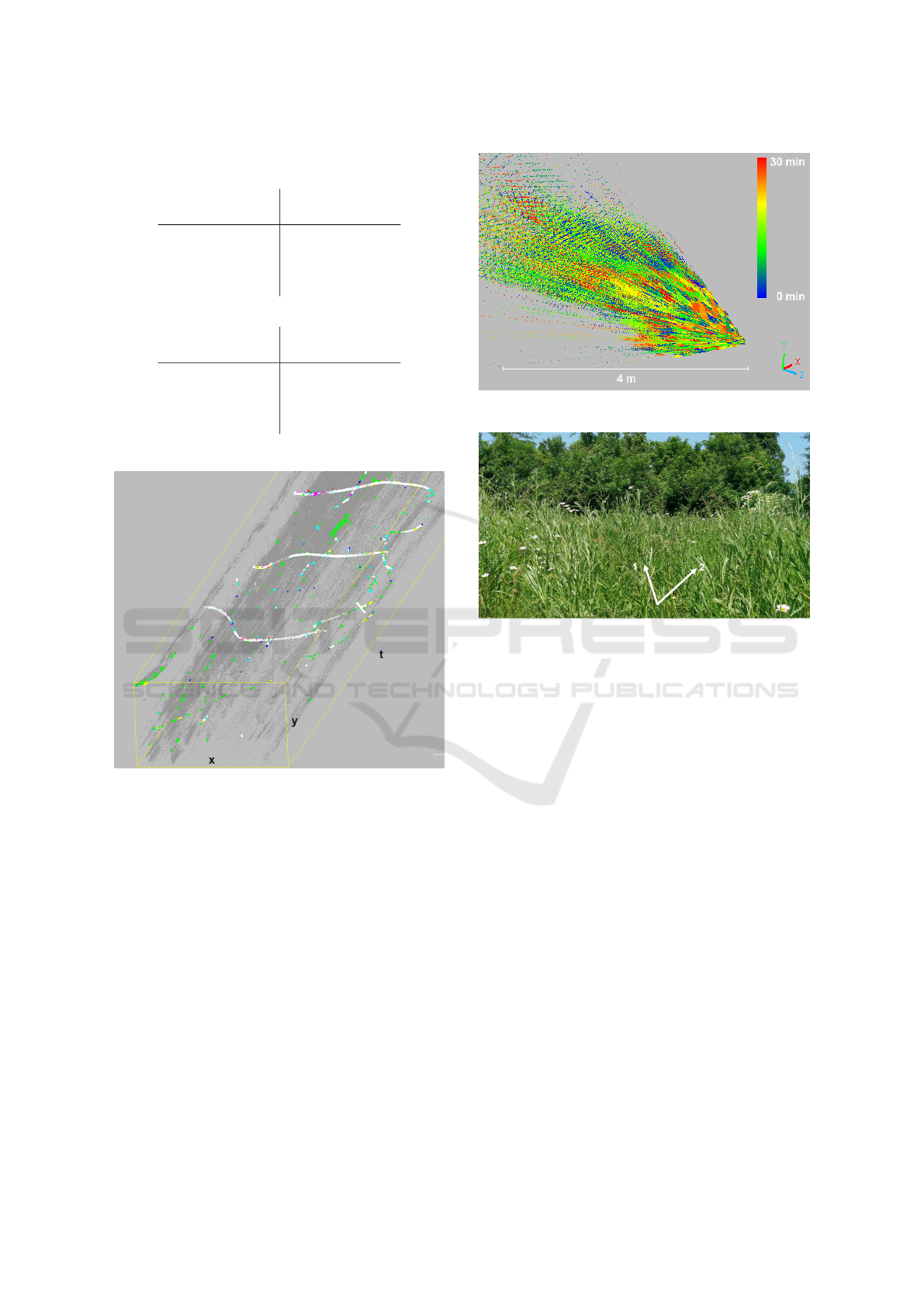
Table 2: Resulting F1 scores for different encoding meth-

ods.

class Environ- Insect

ment

histogram 0.910 0.662

linear time surface 0.500 0.633

event cube 0.891 0.665

optical ﬂow 0.490 0.663

(a) Plain inference after 100 epoch training.

class Environ- Insect

ment

histogram 0.967 0.897

linear time surface 0.956 0.857

event cube 0.912 0.755

optical ﬂow 0.945 0.807

(b) Results after post-processing.

Figure 12: Result of the prediction for the dataset of the

meadow in direction 1 using the different encoding methods

(red: event cube encoding, green: optical ﬂow encoding,

blue: histogram encoding). All other colors result from ad-

ditive color mixing. For the detected environmental events,

a value of 50 was additionally used for the alpha channel.

togram encoding are colored blue. All other colors

result from additive color mixing. Events shown in

white were predicted to be part of the insect ﬂight path

by all three encodings. All black events were clas-

siﬁed as noise or part of the plant movement by all

methods. It can be seen that the optical ﬂow encod-

ing incorrectly predicted many events of plant move-

ment, while the event cube encoding often failed to

detect parts of the insect trajectory. The best results

(blue, white, magenta and cyan markers) are provided

by histogram encoding.

(a) All trajectories in 30 minutes for the meadow in view

direction 1.

(b) Considered meadow with the two directions of view

used.

Figure 13: Detected trajectories in a time interval of 30 min-

utes for the considered meadow shown below.

5.2 Depth Estimation Visualization

The visualization of the data from two 30-minute

recordings of a meadow in two different view direc-

tions is based on the computation of the 4D data us-

ing histogram encoding. Figure 13a shows all in-

sect movements over 30 minutes in the ﬁrst record-

ing. In the displayed view volume, the time is coded

by the color. It can be seen that insect ﬂight occurred

anywhere up to 4 meters in the meadow during the

recording.

Beyond about 4 m from the camera, the data

thinned out, partly due to inaccuracies in the camera

calibration and partly due to the chosen position of

the camera just below the tallest plants (Figure 13b).

The trajectories determined at shorter time intervals

for the two different views of the meadow are shown

in Figure 14 to better assess the quality of the results.

VISAPP 2024 - 19th International Conference on Computer Vision Theory and Applications

382

(a) 25 seconds of the ﬁrst

recording.

(b) 90 seconds of the ﬁrst

recording.

Figure 14: Trajectories of the ﬁrst recording of a meadow

over 25 and 90 seconds and the second recording over 19

seconds.

6 CONCLUSIONS AND FUTURE

WORK

This paper presents the steps of the developed pro-

cessing pipeline from image acquisition to 4D display

for long-term insect monitoring with a stereo event

camera setup. Segmentation results have shown that

insect trajectories can be reliably separated from plant

movements. The use of histogram encoding gave the

best results. To improve the segmentation, besides

the improvement of the dataset a Siamese neural net-

work will be tested, which uses the same weights but

works in parallel on the two different input images to

obtain comparable segmentation results. This could

compensate for differences in segmentation quality

between the left and right camera images.

There are still some inaccuracies in the calcula-

tion of the 4D coordinates. These are caused by the

construction of the measurement system. The align-

ment of the two event cameras changed slightly due to

transport and heat, so that using the calibration data

resulted in an offset of up to 10 lines, depending on

the position of the events in the pixel matrix. A more

mechanically stable setup will be developed in the fu-

ture. For further interpretation of the data, the next

step will be to cluster the individual trajectories and

convert them to spline curves in order to obtain better

3D ﬂight curves. Methods for trajectory tracking will

also be investigated in order to obtain longer sections

and to avoid double counting of insects. Finally, the

individual trajectories will be classiﬁed into different

insect groups based on the ﬂight patterns as proposed

in (Pohle-Fr

ohlich and Bolten, 2023).

REFERENCES

Bjerge, K., Mann, H. M., and Høye, T. T. (2022). Real-time

insect tracking and monitoring with computer vision

and deep learning. Remote Sensing in Ecology and

Conservation, 8(3):315–327.

Bolten, T., Lentzen, F., Pohle-Fr

ohlich, R., and T

onnies,

K. D. (2022a). Evaluation of deep learning based

3d-point-cloud processing techniques for semantic

segmentation of neuromorphic vision sensor event-

streams. In VISIGRAPP (4: VISAPP), pages 168–179.

Bolten, T., Pohle-Fr

ohlich, R., and T

onnies, K. (2023a). Se-

mantic Scene Filtering for Event Cameras in Long-

Term Outdoor Monitoring Scenarios. In Bebis, G.

et al., editors, 18th International Symposium on Vi-

sual Computing (ISVC), Advances in Visual Comput-

ing, volume 14362 of Lecture Notes in Computer Sci-

ence, pages 79–92, Cham. Springer Nature Switzer-

land.

Bolten, T., Pohle-Fr

ohlich, R., and T

onnies, K. D. (2023b).

Semantic segmentation on neuromorphic vision sen-

sor event-streams using pointnet++ and unet based

processing approaches. In VISIGRAPP (4: VISAPP),

pages 168–178.

Bolten, T., Pohle-Fr

ohlich, R., Volker, D., Br

uck, C.,

Beucker, N., and Hirsch, H.-G. (2022b). Visualiza-

tion of activity data from a sensor-based long-term

monitoring study at a playground. In VISIGRAPP (3:

IVAPP), pages 146–155.

Bradski, G. (2000). The OpenCV Library. Dr. Dobb’s Jour-

nal of Software Tools.

Dennis, R., Shreeve, T., Isaac, N., Roy, D., Hardy, P., Fox,

R., and Asher, J. (2006). The effects of visual ap-

parency on bias in butterﬂy recording and monitoring.

Biological conservation, 128(4):486–492.

Dong, S., Du, J., Jiao, L., Wang, F., Liu, K., Teng, Y.,

and Wang, R. (2022). Automatic crop pest detection

oriented multiscale feature fusion approach. Insects,

13(6):554.

Droissart, V., Azandi, L., Onguene, E. R., Savignac, M.,

Smith, T. B., and Deblauwe, V. (2021). Pict: A

low-cost, modular, open-source camera trap system to

study plant–insect interactions. Methods in Ecology

and Evolution, 12(8):1389–1396.

Gallego, G., Delbr

uck, T., Orchard, G., Bartolozzi, C.,

Taba, B., Censi, A., Leutenegger, S., Davison, A. J.,

Conradt, J., Daniilidis, K., et al. (2020). Event-based

vision: A survey. IEEE transactions on pattern anal-

ysis and machine intelligence, 44(1):154–180.

Hallmann, C. A., Sorg, M., Jongejans, E., Siepel, H.,

Hoﬂand, N., Schwan, H., Stenmans, W., M

uller,

A., Sumser, H., H

orren, T., et al. (2017). More

than 75 percent decline over 27 years in total ﬂy-

ing insect biomass in protected areas. PloS one,

12(10):e0185809.

Stereo-Event-Camera-Technique for Insect Monitoring

383

Marcasan, L. I. S., HULUJAN, I. B., Florian, T., Somsai,

P. A., MILITARU, M., Sestras, A. F., Oltean, I., and

Sestras, R. E. (2022). The importance of assessing

the population structure and biology of psylla species

for pest monitoring and management in pear orchards.

Notulae Botanicae Horti Agrobotanici Cluj-Napoca,

50(4):13022–13022.

Pellegrino, N., Gharaee, Z., and Fieguth, P. (2022). Ma-

chine learning challenges of biological factors in in-

sect image data. arXiv preprint arXiv:2211.02537.

Pohle-Fr

ohlich, R. and Bolten, T. (2023). Concept study

for dynamic vision sensor based insect monitoring.

In Radeva, P., Farinella, G. M., and Bouatouch, K.,

editors, Proceedings of the 18th International Joint

Conference on Computer Vision, Imaging and Com-

puter Graphics Theory and Applications, VISIGRAPP

2023, Volume 4: VISAPP, 2023, pages 411–418.

Prophesee (2023a). Documentation metavision sdk. https:

//docs.prophesee.ai/stable/index.html.

Prophesee (2023b). Metavision evaluation kit-3. https://

www.prophesee.ai/event-based-evk-3/.

Qing, Y., Jin, F., Jian, T., XU, W.-g., ZHU, X.-h., YANG,

B.-j., Jun, L., XIE, Y.-z., Bo, Y., WU, S.-z., et al.

(2020). Development of an automatic monitoring sys-

tem for rice light-trap pests based on machine vision.

Journal of Integrative Agriculture, 19(10):2500–2513.

Ratnayake, M. N., Dyer, A. G., and Dorin, A. (2021). To-

wards computer vision and deep learning facilitated

pollination monitoring for agriculture. In Proceedings

of the IEEE/CVF conference on computer vision and

pattern recognition, pages 2921–2930.

Ronneberger, O., Fischer, P., and Brox, T. (2015). U-Net:

Convolutional Networks for Biomedical Image Seg-

mentation. In International Conference on Medical

image computing and computer-assisted intervention,

pages 234–241. Springer.

Sutherland, W. J., Roy, D. B., and Amano, T. (2015). An

agenda for the future of biological recording for eco-

logical monitoring and citizen science. Biological

Journal of the Linnean Society, 115(3):779–784.

agele, J. W., Bodesheim, P., Bourlat, S. J., Denzler,

J., Diepenbroek, M., Fonseca, V., Frommolt, K.-H.,

Geiger, M. F., Gemeinholzer, B., Gl

ockner, F. O., et al.

(2022). Towards a multisensor station for automated

biodiversity monitoring. Basic and Applied Ecology,

59:105–138.

VISAPP 2024 - 19th International Conference on Computer Vision Theory and Applications

384