Packing-Inspired Algorithms for Periodic Scheduling Problems with

Harmonic Periods

Josef Grus

1,4 a

, Claire Hanen

2,3 b

and Zden

ek Hanz

alek

4 c

DCE, FEE, Czech Technical University in Prague, Czech Republic

Sorbonne Universit

e, CNRS, LIP6, F-75005 Paris, France

UPL, Universit

e Paris Nanterre, F-92000 Nanterre, France

IID, CIIRC, Czech Technical University in Prague, Czech Republic

Keywords:

Periodic Scheduling, Harmonic Periods, Height-Divisible 2D Packing, First Fit Heuristic.

Abstract:

We tackle the problem of non-preemptive periodic scheduling with a harmonic set of periods. Problems of this

kind arise within domains of periodic manufacturing and maintenance and also during the design of industrial,

automotive, and avionics communication protocols, where an efﬁcient static schedule of messages is crucial

for the performance of a time-triggered network. We consider the decision variant of the periodic scheduling

problem on a single highly-utilized machine. We ﬁrst prove a bijection between periodic scheduling and a

particular 2D packing of rectangles (we name it height-divisible 2D packing). We formulate the problem

using Constraint Programming and compare it with equivalent state-of-the-art Integer Linear Programming

formulation, showing the former’s superiority on difﬁcult instances. Furthermore, we develop a packing-

inspired ﬁrst ﬁt heuristic, which we compare with methods described in the literature. We justify our proposed

methods on problem instances inspired by the communication of messages on one channel.

1 INTRODUCTION AND

RELATED WORK

Periodic Scheduling Problems (PSPs) often arise

when dealing with manufacturing and maintenance

schedules. Another important application area is the

conﬁguration of communications protocols in the in-

dustrial, automotive, and avionics domains. The con-

ﬁguration is based upon an ofﬂine generated schedule

specifying start times of so-called time-triggered mes-

sages, typically used for safety-relevant functions. It

is important to have an efﬁcient solution because the

demand for communication bandwidth has been in-

creasing signiﬁcantly when messages from a cam-

era, lidar, or radar become a part of safety-relevant

functions in modern self-driving cars (Hanzalek et al.,

2023).

In this paper, we study the decision problem of

scheduling non-preemptive jobs on a single machine,

where the periods of the jobs are harmonic; for any

two distinct periods, it holds that the longer period

https://orcid.org/0000-0002-1136-370X

https://orcid.org/0000-0003-2482-5042

https://orcid.org/0000-0002-8135-1296

is divisible by the shorter one. We assume that the

schedule has to be strictly periodic: the interval be-

tween two occurrences of the same job is equal to the

job period.

PSPs with a harmonic set of periods and process-

ing times are easier to solve than the more general

case (Korst et al., 1996). However, the case with

harmonic periods and non-harmonic processing times

was proven to be strongly NP-complete in (Cai and

Kong, 1996). Schedules with harmonic periods were

applied in many industrial settings. For example,

in FlexRay standard (a communication protocol used

in higher-class cars (Lukasiewycz et al., 2009; Dvo-

rak and Hanzalek, 2014)), we aim to ﬁnd a periodic

schedule for a so-called static segment where the jobs

represent the messages and the machine represents the

physical communication channel. Furthermore, Boe-

ing’s avionics-related problem instances were solved

using methods for harmonic periods in (Eisenbrand

et al., 2010b) as well.

The general PSPs are usually modeled using

time-indexed formulations or relative order formu-

lations, implemented using Integer Linear Program-

ming (ILP) in (Eisenbrand et al., 2010b) or Satisﬁabil-

Grus, J., Hanen, C. and Hanzálek, Z.

Packing-Inspired Algorithms for Periodic Scheduling Problems with Harmonic Periods.

DOI: 10.5220/0012325800003639

Paper published under CC license (CC BY-NC-ND 4.0)

In Proceedings of the 13th International Conference on Operations Research and Enterprise Systems (ICORES 2024), pages 101-112

ISBN: 978-989-758-681-1; ISSN: 2184-4372

101

ity Modulo Theory in (Minaeva and Hanzalek, 2021).

In (Hladik et al., 2020), PSP with harmonic periods,

precedence constraints, and dedicated machines was

tackled using a local search ﬁrst-ﬁt heuristic.

Other methods exploit characteristics of the PSP

with harmonic periods. In this case, the feasible

schedule can be visualized using the bin tree repre-

sentation, shown in (Eisenbrand et al., 2010a), or us-

ing the 2D packing approach described in this paper.

In (Eisenbrand et al., 2010a), authors use the com-

pressed bin trees to develop a ﬁrst ﬁt heuristic to solve

a machine minimization problem. Later in (Eisen-

brand et al., 2010b), the authors presented an alterna-

tive well-performing ILP formulation. Similar ﬁrst ﬁt

heuristic and ILP formulation, used for the FlexRay

bus optimization, were shown in (Lukasiewycz et al.,

2009). In (Dvorak and Hanzalek, 2014), a ﬁrst-

ﬁt-based heuristic was utilized to create a FlexRay

schedule that could be embedded into multiple mod-

els of vehicles. In (Marouf and Sorel, 2011), authors

performed a schedulability analysis of both harmonic

and non-harmonic PSPs.

The crucial correspondence between the PSP with

harmonic periods and the height-divisible 2D packing

problem was outlined in our previous paper (Hanen

and Hanzalek, 2020). This allows us to get inspira-

tion from the algorithms developed for the packing

and cutting problems. In (Fleszar and Hindi, 2002),

authors presented a bin-focused heuristic. A similar

method, generalized for a variable-sized bin packing,

was presented in (Haouari and Serairi, 2009).

In the 2D case, the guillotine cutting and k-stage

packing problems can be considered a generalization

of the height-divisible 2D packing later deﬁned in this

paper. On the other hand, height-divisible 2D pack-

ing is more general than 1D packing. In (Ntene and

van Vuuren, 2009), authors provide the overview of

guillotine heuristics for strip packing and present their

own size alternating stack heuristic, further improved

in (Ortmann et al., 2010). Finally, we can special-

ize the ideas of general packing heuristics, such as the

work of (Crainic et al., 2008) for 3D bin-packing, into

our height-divisible problem environment.

With respect to the relevant research, the main

contributions of our paper are the following:

• We give a new proof of the equivalence of the PSP

with harmonic periods on a single machine and

the height-divisible 2D packing problem, and we

show that any solution obtained for the 2D pack-

ing problem can be transformed into a canonical

form.

• We present a Constraint Programming (CP) for-

mulation of the problem and compare it with the

state-of-the-art ILP model.

• We present a packing-inspired heuristic, which

enables us to solve more highly utilized problem

instances in comparison with baseline methods.

2 PROBLEM DEFINITION

We consider a set of n independent jobs, J

,...,J

to be performed repeatedly on a single machine.

Each job J

is characterized by its integer process-

ing time p

and its integer period T

. Periods be-

long to a harmonic set T

,...,T

r−1

of size r, so that

∀k ∈ {1,...,r − 1}, T

= b

k−1

where b

is an inte-

ger. We deﬁne the least period w = T

, and we deﬁne

the hyper-period

H to be the least common multiplier

of periods. Due to the harmonic nature of the period

set,

H is equal to the longest period T

r−1

Any periodic schedule deﬁnes for each job J

start time f irst

≤ T

of its ﬁrst occurrence. The j-th

occurrence of J

will start at time f irst

+ ( j − 1)T

where j ≥ 1. We consider the existence of a feasible

schedule here. Let o be the starting time of the ﬁrst

job J

with the least period w. We choose o as the

origin. So we deﬁne s

such that:



f irst

− o i f f irst

≥ o

f irst

+ T

− o otherwise

We call time interval [o,o +

H) the ”observation

interval”. Notice that for any integer k ≥ 1, the sched-

ule of time interval [o +(k −1)

H,o + k

H) is the same

as the schedule of the observation interval shifted by

(k − 1)

H time units. In the rest of the paper, we con-

sider without loss of generality that the ﬁrst occur-

rence of a job J

starts at s

in the observation interval.

Let us now decompose s

with respect to the least

period w: s

= u

+ v

· w, with u

< w, and integer v

Also, u

+ p

≤ w, since an occurrence of job J

needs

to ﬁt between two occurrences of J

at o and o + w.

A feasible schedule has to be collision-free. We

call collision between two jobs J

a situation when

two occurrences of these jobs are processed simulta-

neously. An example of the observation interval of

the collision-free schedule is described in Section 3.2

and is shown in Figure 1a.

We denote by B

∏

i=1

, B

= 1, so that:

= B

w. (1)

We can now state the necessary and sufﬁcient con-

dition for a collision to occur in a periodic schedule.

Lemma 1. A periodic schedule induces a collision

between two jobs J

with periods T

such that

≤ α

if and only if the following conditions hold:

< u

+ p

and u

< u

+ p

(2)

ICORES 2024 - 13th International Conference on Operations Research and Enterprise Systems

102

∃κ ∈ N ∩ [0,

), v

= v

+ κB

(3)

Proof. Suppose that the occurrences k, k

′

of J

col-

lide. For this to happen, the two following conditions

must hold:

+ kT

+ p

> s

+ k

′

and s

+ k

′

+ p

> s

+ kT

. (4)

We decompose s

= u

+ v

· w and s

= u

+ v

· w:

+ (v

+ kB

)w + p

> u

+ (v

+ k

′

and

+ (v

+ kB

)w < u

+ (v

+ k

′

)w + p

(5)

⇐⇒ u

+ p

− u

> (v

− v

+ k

′

− kB

and

− v

+ k

′

− kB

)w > u

− u

− p

(6)

As u

+ p

−u

< w and v

are integers, this can

occur only if v

− v

+ k

′

− kB

≤ 0.

Similarly, as u

− u

− p

> −w the second condi-

tion can occur only if v

− v

+ k

′

− kB

≥ 0.

Hence v

− v

+ k

′

− kB

= 0. As B

is a

multiple of B

, there exists an integer κ such that

− v

= κB

, which proves (3).

Now, if this condition holds, then a collision oc-

curs if u

< u

+ p

and u

< u

+ p

, which ﬁnally

proves the lemma.

Utilization η

of a job J

is the proportion of the

time the job uses: η

. The utilization of the

instance is equal to U =

∑

i=1

. Obviously, U is not

greater than 1 in feasible instances.

3 2D PACKING AND PERIODIC

SCHEDULING

In this section, we ﬁrst present a special case of a

2D packing problem and then show the packing prob-

lem associated with a periodic scheduling instance.

Finally, we prove the equivalence between the two

problems by establishing the correspondence between

schedule times and 2D coordinates of rectangles.

3.1 Height-Divisible 2D Packing

Problem

We deﬁne the Height-Divisible 2D (HD2D) packing

problem. An instance of HD2D packing is deﬁned

by n rectangles. Each rectangle R

has width ℓ

and

height h

. These rectangles are to be packed in a 2D

bin of width w and height H. We assume that there are

r different heights H

≥ ··· ≥ H

r−1

, each one divides

H and that they form a harmonic set: each a height H

divides H

if j < k. Note, that H

= H and H

r−1

= 1.

A feasible packing deﬁnes the bottom left corner

coordinates (x

) of the rectangles, so there are no

collisions between two rectangles, and they all ﬁt into

the bin (x

+ ℓ

≤ w, y

+ h

≤ H).

A packing is said to be height divisible if the

height coordinate y

is divisible by the height of the

rectangle:

mod h

= 0.

So, the HD2D packing problem is to ﬁnd a fea-

sible height-divisible packing. We can now state the

conditions of a collision between two rectangles in a

height-divisible packing.

Lemma 2. In a height-divisible packing, a collision

between rectangles R

and R

such that h

≤ h

occurs

iff all following conditions hold:

< x

+ ℓ

, and x

< x

+ ℓ

(7)

≤ y

< y

+ h

, (8)

Proof. Obviously, a collision occurs if:

− ℓ

< x

+ ℓ

(9)

− h

< y

+ h

(10)

Assuming h

≤ h

, h

divides h

and also divides

and y

. Consequently, the inequality y

−h

< y

re-

formulates to y

≤ y

and the other inequalities remain

the same.

3.2 HD2D Packing Instance Associated

with a PSP Instance

We can now deﬁne a 2D packing instance associated

with a periodic scheduling instance with harmonic pe-

riods. Consider an instance I of the scheduling prob-

lem. We deﬁne an associated instance φ(I) of the

HD2D packing problem.

We set H =

= B

r−1

. To each job J

we associate

a rectangle R

of width ℓ

= p

and height h

, to

ﬁt in a bin of width w and height H.

Packing-Inspired Algorithms for Periodic Scheduling Problems with Harmonic Periods

103

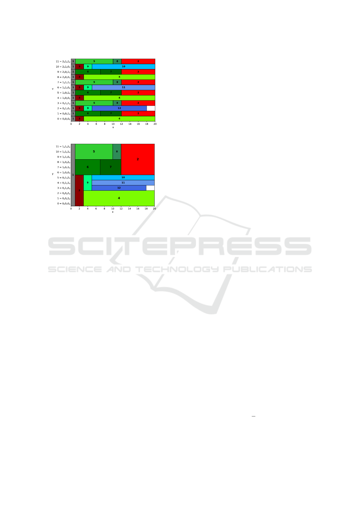
(a) Periodic scheduling problem.

(b) Height-divisible 2D packing problem.

Figure 1: Solutions to PSP and HD2D packing problem,

with corresponding jobs and rectangles presented using the

same colors. Row indices use the mixed-radix system.

To give an intuition of the correspondence be-

tween a periodic schedule and a height-divisible pack-

ing, we ﬁrst develop it on an example in Figures 1.

The main idea is to arrange the periodic schedule in

rows, as shown in Figure 1a. A row indexed by v rep-

resents the schedule of the time window [vw, (v+1)w)

of the observation interval.

The instance contains 12 jobs J

,...,J

. J

is the

only job with the shortest period T

= T

= 20. Jobs

have period equal to 40, jobs J

,...,J

have pe-

riod equal to 80, and ﬁnally, jobs J

have pe-

riod equal to 240. The chart of the periodic schedule

in Figure 1a therefore has width w = T

= 20, and its

height is equal to

H/w = B

= 12. The 2D bin of

the corresponding HD2D packing problem shown in

Figure 1b has the same width w and height H.

Figure 1a shows the chart of the feasible periodic

schedule over a single observation interval of length

= 240. Origin 0 is set by the start time of job J

and we stack each time window of length w = 20 on

top of the previous one (see the rows in Figure 1a with

their three-digit row numbers using mixed-radix sys-

tem formally deﬁned in Section 3.3). We can see that,

e.g., job J

has a period of 80, as its subsequent oc-

currence is at the fourth row from its previous occur-

rence. Note that jobs with the same period use similar

colors.

Figure 1b shows the corresponding height-

divisible packing view of the same solution. The

packing is obtained by interchanging the rows as fol-

lows: we swap the three-digit row numbers in Fig-

ure 1a such that the most signiﬁcant digit becomes

the least signiﬁcant digit and vice versa. Finally, we

obtain Figure 1b by ordering the rows according to

their new three-digit numbers. For example, the row

with J

has number 1

= 6 in Figure 1a and af-

ter the swap, the same row has number 0

= 4 in

Figure 1b.

We can see the occurrences of the original jobs

have been merged, and the dimensions of the result-

ing rectangles correspond to those described in Sec-

tion 3.2. But this is just an observation based on

one example, which does not guarantee a compact

shape of rectangles in HD2D packing. The formal

proof of the equivalence of both problems is derived

in Section 3.3 and uses positions of jobs and rectan-

gles rather than three-digit numbers of rows used in

this Section 3.2.

Note that there exists a bin tree representation of

PSP with harmonic periods. It was used in (Eisen-

brand et al., 2010a) and is closely related to our

HD2D packing perspective. The bin tree represents

the PSP with a tree, with each level of nodes corre-

sponding to one of the periods. Examples of the bin

tree and HD2D packing representations are shown in

Figures 7, 8 in (Minaeva and Hanzalek, 2021).

3.3 Flip Operation and Equivalence

Between HD2D Packing Problem

and PSP

In this section, we will formally introduce a ﬂip oper-

ation, ﬁrst introduced in our paper (Hanen and Han-

zalek, 2020). The ﬂip operation allows us to pro-

vide new proof of a bijection between feasible peri-

odic schedules and HD2D packing of the associated

packing instance in Theorem 1.

Theorem 1. To any periodic feasible schedule of the

instance I, a feasible height-divisible 2D packing of

φ(I) is associated.

∀J



= u

= h

· f lip(v

,α

,b)

(11)

Conversely, from a height-divisible 2D packing of

φ(I) we can deﬁne a feasible schedule as follows:

∀J



= x

= f lip(

,α

,B f (b, α

))

(12)

We ﬁrst introduce the theoretical framework used

to prove Theorem 1. Let y be any natural number.

ICORES 2024 - 13th International Conference on Operations Research and Enterprise Systems

104

It is known that y < H can be decomposed uniquely

according to the mixed radix numerical system b =

,...,b

r−1

) as follows:

y = y

+ y

+ ... + y

r−1

r−2

with ∀i > 0,y

< b

. This decomposition is usually

denoted with the most signiﬁcant digits to the left as

follows:

[y]

= [y

r−1

]

r−1

...[y

]

(13)

Notice that in the usual base decomposition (for

example, base 2 for a binary decomposition), the

components of the base vector b are all equal (for ex-

ample, equal to 2 for the binary decomposition).

Let us generalize the transformation proposed by

(Lukasiewycz et al., 2009) for the binary decompo-

sition of a number by deﬁning two operators: Let

B f (b, k) be the operator that ﬂips the k ﬁrst compo-

nent of the base vector b:

B f (b, k) = (b

k−1

,...,b

k+1

...,b

r−1

) (14)

Let now f lip(y, k,b) be the number constructed

by ﬂipping the k least signiﬁcant digits of the decom-

position [y]

to give a number expressed with respect

to base vector b

′

= B f (b, k):

[ f lip(y, k, b)]

′

= [y

r−1

]

r−1

...[y

k+1

]

k+1

]

...[y

]

(15)

Notice that the r −1 −k most signiﬁcant digits are not

modiﬁed.

Hence, we have:

f lip(y,k, b) = y

·1+y

k−1

·b

+...+y

···b

k+1

···b

) + . . . + y

r−1

···b

r−2

) (16)

Example: consider the base vector b = (2,2,3)

used in Figure 1a. So H = 12. Let us consider y =

10. Its decomposition along b is [y]

= [2]

[1]

[0]

0 + 1 · 2 + 2 · 4. B f (b, 3) = (3,2,2). f lip(y, 3, b) =

[0]

[1]

[2]

= 2 +1 · 3 + 0 · 6 = 5.

This ﬂip operation has some important properties

that will be used to transform the scheduling problem

into an equivalent packing problem. The following

lemma expresses the reversibility of the ﬂip and the

fact that equidistant integers (with distance B

k−1

) be-

come consecutive integers after the ﬂip operation.

Lemma 3. For any integer y < H,

f lip( f lip(y,k, b),k,B f (b, k)) = y (17)

if [y

]

< b

− 1, then

f lip(y + B

k−1

,k, b) = f lip(y,k, b) + 1 (18)

and if [y

]

> 0,

f lip(y − B

k−1

,k, b) = f lip(y,k, b) − 1 (19)

If y is a multiple of B

, z < B

and k

′

≥ k then

f lip(y+z,k

′

,b) = f lip(y,k

′

,b) + f lip(z, k

′

,b) (20)

Proof. Obviously, B f (B f (b,k),k) = b, since a dou-

ble ﬂip of the k ﬁrst digits lead to the initial digits.

This proves (17). Let us consider (18). If we add

k−1

to y, the digit [y

]

increases by one unit, so

after the ﬂip operation, this digit will be the least sig-

niﬁcant; hence, the corresponding number increases

by 1. Similar arguments hold for (19). Finally, if y is

a multiple of B

, its k least signiﬁcant digits are null

with respect to base b. If z < B

its digits from k + 1

to the last one are null, so the sum y + z consists in the

k ﬁrst digits of z followed by the next digits of y. If

′

≥ k f lip(y,k

′

,b) has k

′

− k ﬁrst ﬂipped digits from

the digits k to k

′

of y and f lip(z,k

′

,b) starts with k

′

−k

null digits followed by the ﬂipped k digits of z. So, the

sum is exactly the ﬂipped digits from y + z.

We are now able to prove the equivalence between

PSP and HD2D packing problem.

Proof of Theorem 1.

Proof. The proof relies on the properties of the ﬂip

operation stated in Lemma 3 and the expressions of

collisions stated in Lemma 1 and 2.

Assume that there is a feasible schedule of in-

stance I. Now, assume that a collision occurs in the

associated 2D packing between rectangles R

and R

such that h

≥ h

, so that T

≤ T

So according to equation (7), and as x

= u

we have u

< u

+ p

and u

< u

+ p

. This implies

that the condition (2) of Lemma 1 holds, and thus, as

there is no collision in the schedule, the second condi-

tion cannot hold: v

− v

cannot be a multiple of B

Now according to Lemma 2, equation (9), the col-

lision in the packing implies that:

≤ y

< y

+ h

Assume that y

= y

+ ∆. Notice that as h

divides

, and as h

divides y

, it should also divide ∆. More-

over:

= h

· f lip(v

,α

,b) = h

· f lip(v

,α

,b) + ∆

f lip(v

,α

,b) =

f lip(v

,α

,b) +

∆

with

∆

Now according to Lemma 3,

= f lip(

,α

,B f (b, α

))

= f lip(

f lip(v

,α

,b) +

∆

,α

,B f (b, α

))

Packing-Inspired Algorithms for Periodic Scheduling Problems with Harmonic Periods

105

Observe that

= b

...b

. And

∆

= b

...b

. So applying Lemma 3 with base

B f (b, α

) we can say that:

= f lip(

f lip(v

,α

,b), α

,B f (b, α

))

+ f lip(

∆

,α

,B f (b, α

))

In the base representation B f (b,α

) the α

−

least signiﬁcant digits of

f lip(v

,α

,b) equal

0. And the next α

digits are the ones of v

ﬂipped. So that the α

least signiﬁcant digits of

f lip(

f lip(v

,α

,b), α

,B f (b, α

)) in the base rep-

resentation b are equal to the α

least signiﬁcant dig-

its of v

in base representation b followed by digits 0.

Hence v

= f lip(

f lip(v

,α

,b), α

,B f (b, α

)).

Moreover the number f lip(

∆

,α

,B f (b, α

)) has

its α

least signiﬁcant digits equal to 0 in the base rep-

resentation b. So that it is a multiple of B

= v

+ κB

. (21)

Since we know that v

= B

, we have

κ <

. So condition (3) of Lemma 1 holds, which

contradicts our assumption that no collision occurs.

Conversely, assume that we have a feasible pack-

ing and let us assume that there is a collision in

the associated schedule between jobs J

and J

with

≤ T

. The ﬁrst condition of Lemma 1 holds so

that the ﬁrst condition of Lemma 2 holds either. This

implies that the condition (8) of Lemma 2 does not

hold, and either y

> y

or y

≥ y

+ h

But if a collision occurs in the schedule, we should

have: v

= v

+ κB

So,

= f lip(v

,α

,b)

= f lip(v

+ κB

,α

,b)

= f lip( f lip(

,α

,B f (b, α

)) + κB

,α

,b)

Notice that as y

< H so that

< B

and thus when performing the operation

f lip(

,α

,B f (b, α

)), we get a number still

less than B

. We can then apply Lemma 3, and we

get:

f lip( f lip(

,α

,B f (b, α

)) + κB

,α

,b)

= f lip( f lip(

,α

,B f (b, α

)),α

,b) + κ

+ κ

Now h

= h

= H, so that:

= y

+ κ · h

(22)

Now we know that κ <

. So y

< y

+ h

and condition (8) of Lemma 2 holds, a contradiction.

3.4 Canonical Form of a HD2D Packing

In this section, we prove that any HD2D packing can

be put in a canonical form for which the packed rect-

angles’ heights decrease from the left to the right.

Deﬁnition 1. A height-divisible packing is said to be

in canonical form if for all i, j ∈ {1,...,n}

> h

, y

≥ y

, y

+ h

≤ y

+ h

=⇒ x

+ ℓ

≤ x

(23)

Such a packing corresponds to a schedule of the

observation interval where in each interval [kw,(k +

1)w) (i.e., the k-th row in Figure 1a), jobs are sched-

uled in increasing order of periods.

Theorem 2. If there exists a feasible packing of width

ℓ, then there exists a feasible canonical packing of

width ℓ.

Proof. By induction on r the number of different

heights of rectangles. Of course, if r = 1, the theorem

holds. Assume this is true for any height-divisible

packing with at most r different heights. Consider

an instance with r + 1 different heights. We claim

that the rectangles of maximal height H = H

can be

packed at the left of the bin, and the other rectangles

can be right-shifted accordingly. Let ℓ

′

be the sum of

the lengths of the rectangles of height H

. Consider

the second largest height. If R

is a rectangle of

height h

≤ H

, we know that its vertical coordinate

is a multiple of h

. So there exists a non-negative in-

teger q such that y

= qh

= q

′

+ y

′

, with y

′

≥ 0

and y

′

+ h

≤ H

So we can consider

so-called sub-bins of

height H

and width ℓ−ℓ

′

in which all remaining rect-

angles are packed. Here, rectangle R

is packed in

sub-bin q

′

. The set of rectangles packed into a sub-

bin has at most r different heights. By induction, all

the rectangles packed in a sub-bin can be packed with

a canonical packing.

The canonical form of the packing shown in Fig-

ure 1b is presented in Figure 2. The canonical form

also shows sub-bins, which are crucial for the descrip-

tion of heuristics. The original 2D bin of size w × H

starts from the left as a single sub-bin of height H.

Once all rectangles with height H

= H are packed

ICORES 2024 - 13th International Conference on Operations Research and Enterprise Systems

106

Figure 2: Canonical form of the packing shown in Fig-

ure 1b. Sub-bin division is highlighted by special T-like

guillotine cuts in gray, red, and green colors, that are appli-

cable in the canonical form only.

(grey rectangle R

in Figure 2), the remaining free

space to the right of the parent sub-bin is divided to

sub-bins of height H

. Once rectangles with height

are packed (reddish rectangles R

), we divide

each sub-bin into

sub-bins of height H

. This con-

tinues until sub-bins of height H

r−1

= 1 are created,

and the rectangles with the smallest height are packed.

In Figure 2, the lower sub-bin of height 6 con-

tains rectangles R

. The division

of sub-bins is also highlighted by the colored T-like

contours. For example, the sub-bin of height 6, where

rectangle R

is packed, divides itself into two sub-

bins, each containing two rectangles of height 3.

4 CP MODEL

We use the bin formulation, found in (Lukasiewycz

et al., 2009; Eisenbrand et al., 2010b), to model and

solve the single machine PSP with harmonic periods.

We formulate the problem from the HD2D packing

perspective, and the solution to the PSP is obtained

using the equations from Section 3.3. The bin for-

mulation only assigns the rectangles to suitable sub-

bins, as described in the previous section. Once such

an assignment is obtained, the packing solution in the

canonical form is recovered.

We model the bin formulation using CP. We rely

on the pack constraint (Shaw, 2004). The constraint

pack(L,a,l) couples together list L of groups’ load

variables, list a of items’ assignment variables, and

list l of items’ sizes, so:

∈ {0,...,|L| −1} ∀i ∈ {0, . ..,|a|− 1} (24)

∑

∀ j :a

∀i ∈ {0,...,|L| − 1} (25)

Thus, each item is assigned to one of the groups,

and each group’s load variable contains the sum of its

assigned items’ sizes.

To model the HD2D packing problem, we use one

pack constraint for each distinct height H

. This pack

constraint uses load variables L

= (L

,...,L

−1

)

to model

sub-bins of height H

. The sub-bins are

indexed from bottom to top. Lists of widths l

and

assignment variables a

are associated with all rect-

angles with height h

= H

. With these deﬁnitions,

the used pack constraints are:

pack(L

) ∀k ∈ {0, . . . , r −1} (26)

Such constraint distributes the rectangles with

height H

among sub-bins with height H

, and the

load variable L

is equal to the sum of widths of rect-

angles that are assigned to i-th sub-bin of height H

Then, for each row of height 1 in the packing, we sum

together loads of sub-bins that intersect such row (see

Figure 2). We ensure that such sum does not exceed

the width of the 2D bin w:

r−1

∑

k=0

⌊i/H

⌋

≤ w ∀i ∈ {0,...H

− 1} (27)

In the case of line 4 in Figure 2 we sum up L

= 1

plus L

= 2 plus L

= 15.

These two sets of constraints are sufﬁcient to

model the problem. Once solved, the assignment of

rectangles to sub-bins is determined from values of

variables a

5 HEURISTICS

While the exact approaches completely search the so-

lution space, their performance diminishes with an in-

creasing number of jobs to schedule. On the other

hand, even simple heuristics are often able to ﬁnd a

solution for large instances (Hladik et al., 2020).

All studied heuristics process the jobs one by

one, ordered ﬁrst non-decreasingly by their period

and then non-increasingly by their processing times.

The period ordering (known as rate-monotonic in the

time-triggered community) is natural, several heuris-

tics rely on it, and it produces a solution in canonical

form. The secondary ordering by processing times is

used by the bin packing and scheduling approxima-

tion algorithms (e.g., in (Della Croce and Scatamac-

chia, 2018)).

5.1 Baseline Heuristics

5.1.1 Time-Wise First Fit

In (Hladik et al., 2020), authors originally tackled

the problem with dedicated machines and precedence

Packing-Inspired Algorithms for Periodic Scheduling Problems with Harmonic Periods

107

constraints. Their algorithm schedules each job as

soon as possible, minimizing the job’s start time in

the yet-unﬁnished schedule. Due to the time-oriented

aspect of the heuristic, we denote it T-FF.

5.1.2 Spatial First Fit and Best Fit

In (Eisenbrand et al., 2010a), the ﬁrst ﬁt is also used.

However, the rectangles of the corresponding HD2D

packing problem are packed to the lowest available

sub-bin instead. We refer to this approach as a spa-

tial ﬁrst ﬁt. Furthermore, we also tested best ﬁt as a

sub-bin selection policy; thus, we obtained two dis-

tinct variants of the algorithm, denoted S-FF and S-

BF respectively. Note that the best-ﬁt selection can be

viewed as a single-dimension ”Residual Space” merit

function, used to pack items in (Crainic et al., 2008).

5.1.3 Longest Processing Time First

The last baseline approach is the well-known Longest

Processing Time First list scheduling algorithm for

parallel machines scheduling (Della Croce and Scata-

macchia, 2018). We follow the same spatial approach

of Section 5.1.2, but for the current job, its corre-

sponding rectangle is packed into the least occupied

sub-bin. We denote this method LPT.

5.2 Rectangle-Guided First Fit

We observed that the baseline heuristics often cannot

schedule infrequent long jobs, whose corresponding

rectangles are wide and low. These rectangles are

packed later in the process when the packing is mostly

ﬁlled. Following this observation, we designed our

heuristic, called rectangle-guided ﬁrst ﬁt, using the

HD2D packing perspective. The algorithm consists

of two phases. In the ﬁrst phase, so-called dummy

rectangles are created, and in the second phase, the

rectangles (including dummy rectangles) are packed

using a modiﬁed ﬁrst ﬁt heuristic.

Partly inspired by ”wide” and ”narrow” rectan-

gles of (Ntene and van Vuuren, 2009; Ortmann et al.,

2010), the dummy rectangles are created for each dis-

tinct height H

of the problem. For H

r−1

= 1, there are

no dummy rectangles. For each subsequent height H

the dummy rectangles are constructed based on both

real and dummy rectangles of height H

k+1

. As the

newly created rectangles are taller, they will be pro-

cessed earlier by the heuristic and will reserve space

for the smaller ones. However, their only purpose is

to provide a look-ahead; once all the rectangles with

height H

are packed, we remove all the dummy rect-

angles with height H

from the sub-bins and continue

with packing the rectangles of height H

k+1

(a) Pessimistic construction.

(b) Optimistic construction.

Figure 3: Bag view of dummy rectangles for height H

= 6

constructed for instance from Section 3.2.

5.2.1 On Construction of Dummy Rectangles

Dummy rectangle of height H

and width l essen-

tially consists of H

k+1

bins of height H

k+1

, each

with width l. Our aim is to create dummy rectan-

gles by ﬁlling these bins with the smaller rectangles

of height H

k+1

, so the new rectangles roughly cap-

ture how the smaller rectangles could be packed. We

create the rectangles heuristically using 1D bin pack-

ing. To avoid confusion with the 2D packing, we call

the one-dimensional bins bags. We propose two ap-

proaches for constructing dummy rectangles.

The pessimistic approach sorts the rectangles with

height H

k+1

by their width. We start with an empty

list of bags. If a rectangle R

with width l

ﬁts in one

of the existing bags, it is packed according to the best

ﬁt policy. If not, a new dummy rectangle of height H

is created, with width l

. Simultaneously, H

k+1

bags of size l

are created, and R

fully ﬁlls one of

them. The process repeats until all the rectangles are

packed in the bags. Since many bags may contain

holes, not all constructed dummy rectangles are com-

pletely ﬁlled with the smaller ones. This is shown in

Figure 3a. Three dummy rectangles of height 6 were

created from rectangles of height 3, but two bags as-

sociated with two narrower rectangles were not fully

ﬁlled. Note that the blue rectangle is the dummy rect-

angle created for H

= 3. We refer to our algorithm

using pessimistic construction as RG-FF-PES.

The optimistic variant ﬁlls the bags in a ”preemp-

tive manner” and always keeps at most a single bag

not full. We start with an empty list of bags. Until

we exhaust all the rectangles with height H

k+1

, we

select the widest R

with width l

. If it ﬁts any (i.e.,

the single not full) bag, we pack it to it. If the bag has

ICORES 2024 - 13th International Conference on Operations Research and Enterprise Systems

108

(a) T-FF. (b) S-FF. (c) RG-FF-OPT.

Figure 4: Unﬁnished (a), (b) and ﬁnished (c) packings created by different methods on instance from Section 3.2.

vacant size 0 < A < l

, we split R

into two rectangles

with widths A and l

−A. The ﬁrst rectangle is packed

into the bag, and the second is pushed back among

the remaining rectangles. If all the bags are full, we

create a new dummy rectangle of height H

and width

, push a new bag with size l

· H

k+1

to the list of

bags, and pack R

into it; this new bag is a concate-

nation of H

k+1

bags of width l

, that make up the

rectangle. We denote this variant of the algorithm as

RG-FF-OPT.

Note that only the last bag might contain holes.

In Figure 3b, all the bags were actually fully ﬁlled.

Also, notice that rectangles R

were split into two

parts. Due to the splitting and the usage of a sin-

gle rather than H

= 2 bags, we cannot simply

partition the packed dummy rectangle into a feasible

packing of rectangles that ﬁlled the associated bag;

in a pessimistic case, it is possible (see Figure 3a).

However, since the dummy rectangles only provide a

look-ahead, this ”preemptiveness” does not cause is-

sues with the ﬁnal packing.

5.2.2 First Fit Packing

Once the dummy rectangles are constructed, our al-

gorithm follows the ﬁrst ﬁt approach of algorithm

S-FF. All the rectangles, both real and dummy,

are sorted following the policy of Section 5; ﬁrst,

non-increasingly by height, then non-increasingly by

width.

Our algorithm differs from S-FF in two ways.

Once the last rectangle of height H

is packed, we

remove packed dummy rectangles from all the sub-

bins, recalculate the sub-bins’ utilizations, and then

continue packing the rectangles of height H

k+1

. The

second difference is the packing policy. If the cur-

rent rectangle R

ﬁts any sub-bin, we pack it accord-

ing to the ﬁrst ﬁt policy. If not, we do not im-

mediately stop the algorithm; the sub-bins may be-

come under-utilized once the dummy rectangles are

removed. Thus, if R

is a dummy rectangle, we pack

it to the least utilized sub-bin, temporarily exceeding

the sub-bin’s size. If R

is a real rectangle, we ﬁnd

the sub-bins that would ﬁt R

after removal of dummy

rectangles. If such sub-bins exist, we pack R

to the

least utilized one; otherwise, the heuristic fails to ﬁnd

a feasible solution. If all real rectangles are packed,

the algorithm ﬁnishes successfully, and we transform

the packing into the schedule.

Internally, we use the compressed bin tree repre-

sentation of (Eisenbrand et al., 2010a) so the com-

plexity of the ﬁrst ﬁt packing of a single rectangle is

O(n) given n rectangles to pack (i.e., jobs to sched-

ule). Since for each height H

we need to process

O(n) real and dummy rectangles, the overall com-

plexity of our solution is O(r · n

5.3 Comparison of Methods

In Figures 4, we compare T-FF, S-FF, and RG-FF-

OPT methods on example instance from Section 3.2,

using the HD2D packing view. Neither T-FF nor S-

FF methods were successful, as they were not able to

reserve space for blue rectangle R

. Notice that T-

FF and S-FF put rectangle R

to different sub-bins.

While both methods process R

at the same moment,

T-FF selects the time-wise earliest start time for the

associated job, while S-FF selects the lowest sub-

bin. Finally, RG-FF-OPT used dummy rectangles

to reserve enough space for R

by putting rectangles

into different sub-bins.

6 EXPERIMENTS

The algorithms were implemented in Python 3.10.

Experiments were performed on an Intel Xeon Sil-

ver 4110@2.10 GHz, using IBM ILOG CP Optimizer

v22.1.1 and Gurobi v10.0.2.

6.1 Experimental Data

We evaluated the methods on several sets of syntheti-

cally generated problem instances. Due to the success

of the method by (Hladik et al., 2020), we only gen-

Packing-Inspired Algorithms for Periodic Scheduling Problems with Harmonic Periods

109

Table 1: Number of instances solved by each method on instance sets S

heuristic exact

set # instances LPT T-FF S-FF S-BF RG-FF-PES RG-FF-OPT ILP CP

3518 2213 3233 3248 3263 3378 3378 3518 3518

800 122 558 562 563 681 694 800 800

297 8 14 15 15 24 29 289 289

Table 2: Characteristics of the instance sets.

set # instances average jobs median η

[%] median p

[%]

3518 84 0.098 0.40

800 57 1.563 6.25

297 47 1.719 9.10

200 84 0.278 3.50

200 405 0.028 3.25

200 3719 0.001 3.00

200 1473 0.019 6.88

erated feasible instances with utilization U equal to

100 %.

The ﬁrst sets of instances were generated using the

scheme proposed in (Hladik et al., 2020). Starting

with a selected period T

, a single job with period and

processing time equal to T

is generated. Then, for a

given number of iterations, one of the jobs with period

= T

is selected and is either split into two new

jobs of the same period but shorter processing times

or is divided into b

k+1

jobs with the same processing

time and period equal to T

k+1

Set S

contains original instances from (Hladik

et al., 2020). The original generation scheme of-

ten created instances with many long-period short-

processing times jobs that are relatively easy to solve.

We modiﬁed the generator scheme to account for this

and produced sets S

, and S

Then, we generated 4 sets of difﬁcult instances us-

ing HD2D packing perspective (in canonical form).

We ensured that the majority of jobs had a process-

ing time greater than 13. These short-jobs-free in-

stances seemed to be the most difﬁcult to solve; their

sets were labeled by the letter D. Four sets with 200

instances were created. Each instance set D

used pe-

riod set {800 · T

| k ∈ 0,...,r − 1}.

Characteristics of the instance sets are shown in

Table 2. We show the number of generated instances

and the average number of jobs in the instance. Me-

dian η

is the median utilization across all the jobs of

the instance set. Similarly, median p

is the me-

dian value of the processing time of the job, normal-

ized by the minimum period T

of the associated in-

stance. We can see that the simpler instances contain

only around 80 jobs. However, thanks to their diverse

characteristics, we use them to thoroughly compare

our heuristics.

6.2 Success Rates of the Methods

First, we evaluated how many instances each method

can successfully solve. CP and ILP solvers were lim-

Table 3: Number of instances solved by exact methods on

difﬁcult instance sets.

set # instances ILP CP

200 95 152

200 1 36

200 0 0

Table 4: Number of instances solved by RG-FF-OPT and

combinations of heuristics M

on instance sets S

set # instances RG-FF-OPT M

3518 3378 3423 3439 3437 3459

800 694 709 726 725 742

297 29 30 30 30 33

ited to 3 minutes of computation time per instance.

We found that the heuristics could not ﬁnd any

feasible solutions in the case of the difﬁcult D

in-

stances. Thus, we only used these instances to com-

pare CP and ILP. As is reported in Table 1 both solvers

can solve smaller instances S

. However, CP is

more successful on the mentioned difﬁcult instances

shown in Table 3, given the limited computation time

of 3 minutes. We suspect that the reason is an ef-

ﬁcient formulation that relies on the powerful pack

constraint. However, for difﬁcult sets D

, D

, nei-

ther method found any solution. We use these sets

later in Section 6.3 to highlight the shortcomings of

the CP in comparison with heuristics.

The results of heuristics on sets S

are also

reported in Table 1. We can see that on all these sets,

the packing-inspired methods RG-FF-PES and RG-

FF-OPT defeated the baseline heuristics, with the op-

timistic variant RG-FF-OPT being the best. This is

most pronounced for set S

. Our revised generation

scheme made the instances harder to solve; this was

highlighted by set S

, where heuristics solved only a

few instances. Finally, except for LPT, the results of

baseline heuristics do not differ signiﬁcantly.

We were also interested in the possible orthogo-

nality of the studied heuristics; if each type of the

heuristic would solve a distinct subset of the in-

stances, we could run them as a portfolio and achieve

a higher overall success rate. For each pair of heuris-

tics, we determined the number of instances of the

instance set solved by at least one heuristic from the

pair, and we present several interesting combinations.

is combination of RG-FF-OPT and RG-FF-PES,

is combination of RG-FF-OPT and S-BF, and M

ICORES 2024 - 13th International Conference on Operations Research and Enterprise Systems

110

Table 5: Results of the utilization experiment on instance sets S

heuristic exact

LPT T-FF S-FF S-BF RG-FF-PES RG-FF-OPT CP10 CP60

set # instances # succ avg U

# succ avg U

3518 3452 0.962 3512 0.994 3512 0.995 3512 0.995 3518 0.998 3518 0.998 3518 0.999 3518 0.999

800 788 0.923 798 0.988 798 0.989 798 0.989 800 0.997 800 0.996 800 1.000 800 1.000

297 277 0.915 296 0.964 296 0.965 296 0.966 297 0.978 297 0.977 297 1.000 297 1.000

is combination of RG-FF-OPT and T-FF. Finally, M

corresponds to running all the heuristics together.

From the results reported in Table 4, we can see

that the combination of the two proposed methods

does not offer much improvement. On the other hand,

when we use our heuristic with the S-BF (M

), the re-

sults are signiﬁcantly better, increasing the number of

successes by 30 in the case of set S

. However, set

remains problematic for heuristics to solve, even

when we would run all the heuristics together (M

6.3 Utilization Experiment

While the results reported in Section 6.2 show the

power of the CP, we also studied how each method

tackles the instances with utilization U < 1.0. While

the heuristics have trouble solving instances with

U = 1.0, they might be successful when U is slightly

lower. We study this in the following experiment.

For a given method and instance, we evaluate

whether the method successfully solves the instance.

If not, we remove the job with the smallest value of

utilization η

and repeat the process. When the suc-

cess eventually occurs, we report the ﬁnal utilization

of the instance. Thus, if the method solved each

instance immediately or just after a few iterations, it

would report all the values U

close to 1. Note that

the jobs are removed in a deterministic way, as out-

lined; there might exist a situation when removing

a single longer job would make the instance easier

than removing several shorter jobs consecutively. We

remove the jobs until the utilization of the instance

reaches U < 0.7 when the failure is reported. The ex-

periment was performed for each instance set using

all the heuristics, as well as the CP solver with a time

limit: CP10 was limited to 10 seconds of computa-

tion, while CP60 was limited to 60 seconds.

The number of successes (i.e., number of in-

stances for which success occurred before U

< 0.7)

and an average value of U

of successful attempts on

instance sets S

are shown in Table 5. All the

heuristics, with the exception of the LPT, are able to

solve most of the instances with just a slight reduction

of their overall utilization. This matches the results re-

ported in (Hladik et al., 2020). On instance sets S

(see Figure 5), which were generated with our modi-

ﬁed scheme, the proposed heuristics RG-FF-PES and

RG-FF-OPT report average value of U

1 % higher

Figure 5: Utilization experiment on instance set S

. Colored

dots mark ﬁnal utilizations U

for each instance. Black dots

mark the average value per method.

Figure 6: Utilization experiment on instance set D

. Col-

ored dots mark ﬁnal utilizations U

for each instance. Black

dots mark the average value per method.

than achieved by their baseline counterparts (with the

theoretical maximum being 3 %). These results again

suggest that the proposed methods perform better on

the instances with infrequent long jobs.

Results on difﬁcult sets D

are reported in Table 6.

Interestingly, most heuristics are able to solve them

once the instances’ utilization slightly drops. Regard-

ing the performance of the CP solver, interesting re-

sults are reported for the largest instances of D

There, the performance of CP10 and CP60 diminishes

in contrast with heuristics (whose runtime is at most

0.2 seconds), as is also shown in Figure 6. Thus, as

the instance size grows and with a limited computa-

tion time, it may be better to use heuristics to create a

slightly less utilized schedule.

7 CONCLUSION

In this paper, we studied the PSP with a harmonic set

of periods and non-preemptive jobs on a single ma-

chine. We formally proved that the studied problem

is equivalent to the HD2D packing problem and that

each feasible schedule and its associated packing can

Packing-Inspired Algorithms for Periodic Scheduling Problems with Harmonic Periods

111

Table 6: Results of the utilization experiment on difﬁcult instance sets.

heuristic exact

LPT T-FF S-FF S-BF RG-FF-PES RG-FF-OPT CP10 CP60

set # instances # succ avg U

# succ avg U

200 188 0.873 200 0.995 200 0.994 200 0.995 200 0.994 200 0.992 200 1.000 200 1.000

200 139 0.805 200 0.996 200 0.996 200 0.996 200 0.997 200 0.996 200 0.999 200 1.000

200 61 0.755 200 0.997 200 0.997 200 0.997 200 0.998 200 0.998 144 0.937 200 0.986

200 0 - 200 0.997 200 0.997 200 0.997 200 0.997 200 0.996 200 0.991 200 0.997

be transformed into the canonical form. We used the

CP with a bin formulation and showed its effective-

ness compared to the ILP. Then, we proposed heuris-

tics based on the HD2D packing perspective, suitable

for scheduling instances with infrequent long jobs.

We have shown the advantages of our method in

comparison with several baseline heuristics on sets

of synthetically generated instances. Furthermore,

we performed an experiment where we incrementally

lowered the utilization of instances. The experiments

allowed us to compare the heuristics and observe the

CP’s shortcomings when limited computation time

is in place. The experiments have shown that the

short-jobs-free instances with 100 % utilization are

the most difﬁcult to solve. However, rate-monotonic-

based heuristics work very well whenever the utiliza-

tion slightly drops. The empty space of 99% utiliza-

tion instance behaves as infrequent, very short jobs,

which can ﬁll the fragmented space left at the end of

the constructive heuristics run.

We aim to use the presented results and heuristics

as a basis of evolutionary algorithms to tackle more

complex problems with dedicated machines, prece-

dence relations, and a criterion to optimize.

ACKNOWLEDGEMENTS

This work was supported by the Grant Agency of

the Czech Technical University in Prague, grant

No. SGS22/167/OHK3/3T/13.

This work was co-funded by the European

Union under the project ROBOPROX - Robotics

and advanced industrial production (reg. no.

CZ.02.01.01/00/22 008/0004590).

REFERENCES

Cai, Y. and Kong, M. (1996). Nonpreemptive scheduling

of periodic tasks in uni- and multiprocessor systems.

Algorithmica, 15(6):572–599.

Crainic, T. G., Perboli, G., and Tadei, R. (2008). Extreme

point-based heuristics for three-dimensional bin pack-

ing. INFORMS J. Comput., 20:368–384.

Della Croce, F. and Scatamacchia, R. (2018). Longest pro-

cessing time rule for identical parallel machines revis-

ited. Journal of Scheduling, 23/2:163–176.

Dvorak, J. and Hanzalek, Z. (2014). Multi-variant time

constrained FlexRay static segment scheduling. 2014

10th IEEE WFCS, pages 1–8.

Eisenbrand, F. et al. (2010a). Scheduling periodic tasks in

a hard real-time environment. Automata, Languages

and Programming, 6198:299–311.

Eisenbrand, F. et al. (2010b). Solving an avionics real-time

scheduling problem by advanced IP-methods. Euro-

pean Symposium on Algorithms, pages 11–22.

Fleszar, K. and Hindi, K. S. (2002). New heuristics for one-

dimensional bin-packing. Comput. Oper. Res., 29(7).

Hanen, C. and Hanzalek, Z. (2020). Periodic scheduling

and packing problems. CoRR, abs/2011.01898.

Hanzalek, Z., Zahora, J., and Sojka, M. (2023). Cone

slalom with automated sports car – trajectory planning

algorithm. IEEE Trans. on Vehicular Technology.

Haouari, M. and Serairi, M. (2009). Heuristics for the vari-

able sized bin-packing problem. Comput. Oper. Res.,

36(10).

Hladik, R., Minaeva, A., and Hanzalek, Z. (2020). On

the complexity of a periodic scheduling problem with

precedence relations. In Proc. of COCOA 2020.

Korst, J., Aarts, E., and Lenstra, J. K. (1996). Scheduling

periodic tasks. INFORMS J. Comput., 8(4):428–435.

Lukasiewycz, M. et al. (2009). FlexRay schedule optimiza-

tion of the static segment. In Proc. of IEEE/ACM

CODES+ISSS 2009, pages 363–372.

Marouf, M. and Sorel, Y. (2011). Scheduling non-

preemptive hard real-time tasks with strict periods. In

ETFA2011, pages 1–8.

Minaeva, A. and Hanzalek, Z. (2021). Survey on periodic

scheduling for time-triggered hard real-time systems.

ACM Comput. Surv., 54(1).

Ntene, N. and van Vuuren, J. H. (2009). A survey and com-

parison of guillotine heuristics for the 2D oriented of-

ﬂine strip packing problem. Discrete Optimization,

6(2):174–188.

Ortmann, F. G., Ntene, N., and van Vuuren, J. H. (2010).

New and improved level heuristics for the rectangu-

lar strip packing and variable-sized bin packing prob-

lems. EJOR, 203(2):306–315.

Shaw, P. (2004). A constraint for bin packing. In Interna-

tional Conference on Principles and Practice of Con-

straint Programming.

ICORES 2024 - 13th International Conference on Operations Research and Enterprise Systems

112