Efﬁciency Optimization Strategies for Point Transformer Networks

Jannis Unkrig

and Markus Friedrich

Department of Computer Science and Mathematics, Munich University of Applied Sciences, Munich, Germany

Keywords:

3D Point Cloud Processing, 3D Computer Vision, Deep Learning, Transformer Architecture.

Abstract:

The Point Transformer, and especially its successor Point Transformer V2, are among the state-of-the-art ar-

chitectures for point cloud processing in terms of accuracy. However, like many other point cloud processing

architectures, they suffer from the inherently irregular structure of point clouds, which makes efﬁcient process-

ing computationally expensive. Common workarounds include reducing the point cloud density, or cropping

out partitions, processing them sequentially, and then stitching them back together. However, those approaches

inherently limit the architecture by either providing less detail or less context. This work provides strategies

that directly address efﬁciency bottlenecks in the Point Transformer architecture, and therefore allows process-

ing larger point clouds in a single feed-forward operation. Speciﬁcally, we propose using uniform point cloud

sizes in all stages of the architecture, a k-D tree-based k-nearest neighbor search algorithm that is not only ef-

ﬁcient on large point clouds, but also generates intermediate results that can be reused for downsampling, and

a technique for normalizing local densities which improves overall accuracy. Furthermore, our architecture is

simpler to implement and does not require custom CUDA kernels to run efﬁciently.

1 INTRODUCTION

As shown by Convolutional Neural Networks (CNNs)

(Lecun et al., 1998) or modern Vision Transform-

ers (Liu et al., 2021), respecting locality is instru-

mental for efﬁcient and accurate processing of vi-

sual data. This locality is not implicitly given in 3D

point clouds. As a consequence, locality needs to

be restored explicitly by computationally expensive k

Nearest Neighbor (knn) searches (Zhao et al., 2020b;

Wu et al., 2022), or by determining if a given point is

within a given window (Lai et al., 2022; Yang et al.,

2023). The lack of implicit locality also poses a chal-

lenge for efﬁcient downsampling methods.

The Point Transformer (Zhao et al., 2020b) and

its version 2 (Wu et al., 2022) are among the state-

of-the-art point cloud processing neural network ar-

chitectures. In most cases the authors handled the

expensive, but necessary operations described above

with high efﬁciency custom CUDA kernels. While

these provide a signiﬁcant speed up, they do not di-

rectly address the underlying complexity and thus do

not allow for scaling the models efﬁciency beyond a

given point. Also, they are cumbersome to use and

adapt. For point clouds larger than the default size,

https://orcid.org/0009-0004-9930-4481

https://orcid.org/0000-0001-5719-3198

the authors split each cloud into smaller partitions and

process these sequentially, reduce the density in a pre-

processing step, or use a combination of both. All of

these approaches limit the architecture by either pro-

viding less context or less detail.

In this work, we aim to improve the efﬁciency

of the Point Transformer architecture by directly ad-

dressing bottlenecks, while simultaneously preserv-

ing accuracy — accomplished without the need for

custom CUDA kernels. We thereby not only work to-

wards a faster model, but also towards training and

inference on larger point clouds. Furthermore, we an-

alyze some of the changes proposed in the follow-up

paper and examine their impact on both speed and ac-

curacy.

This paper is organized as follows: Chapter 2 ex-

plores related architectures for point cloud process-

ing. In Chapter 3, we discuss the Point Transformer

architecture our work is based on. The proposed im-

provements are detailed in Chapter 4 and evaluated in

Chapter 5. Chapter 6 presents an ablation study. Fi-

nally, in Chapter 7, we discuss the results and outline

future work.

Unkrig, J. and Friedrich, M.

Efﬁciency Optimization Strategies for Point Transformer Networks.

DOI: 10.5220/0012325000003660

Paper published under CC license (CC BY-NC-ND 4.0)

In Proceedings of the 19th International Joint Conference on Computer Vision, Imaging and Computer Graphics Theory and Applications (VISIGRAPP 2024) - Volume 3: VISAPP, pages

65-76

ISBN: 978-989-758-679-8; ISSN: 2184-4321

2 RELATED WORK

2.1 Point Cloud Processing

There are various learning-based approaches for pro-

cessing 3D point clouds. These methods can be

roughly classiﬁed into three types: projection-based,

voxel-based, and point-based networks. When deal-

ing with irregular inputs contains an ablation study.

like point clouds, a common strategy is to convert the

irregular representations into regular ones.

2.1.1 Projection-Based Networks

Projection-based methods involve projecting 3D point

clouds onto different image planes, and utilizing 2D

CNNs as backbones to extract feature representations

(Su et al., 2015; Chen et al., 2016). These approaches

generally do not utilize the sparsity of point clouds

when forming dense pixel grids on projection planes.

Also the choice of projection planes can heavily in-

ﬂuence performance and occlusion in 3D scenes or

objects is a major problem.

2.1.2 Voxel-Based Networks

Another approach involves performing convolutions

in 3D by transforming irregular point clouds into

regular voxel representations (Maturana and Scherer,

2015). However, voxel-based methods also suffer

from inefﬁciency due to the sparse nature of point

clouds, although this challenge has been addressed

to some extent with the introduction of sparse con-

volution techniques (Graham et al., 2017; Choy et al.,

2019).

2.1.3 Point-Based Networks

Lastly, point-based methods extract features directly

from the point cloud itself, without the need for pro-

jection or quantization onto regular 2D or 3D grids.

PointNet(Qi et al., 2016), was one of the ﬁrst deep

neural network architectures designed for directly

processing point clouds. It employs permutation in-

variant operators such as pointwise MLPs and pool-

ing layers to aggregate features across a point cloud.

Its Successor PointNet++ (Qi et al., 2017) added a hi-

erarchical structure with increasing levels of abstrac-

tion. This signiﬁcantly improved the segmentation

accuracy and robustness and is used in most architec-

tures to this day. Later, a subcategory of point-based

architectures that leverages the connectivity informa-

tion among points by constructing a graph representa-

tion of the point cloud, was proposed in (Wang et al.,

2018). It employs graph convolutional layers to en-

able effective point cloud segmentation. More recent

graph-based approaches are competitive to this day

(Robert et al., 2023).

2.2 Transformers

After the rise of Transformer architectures for natu-

ral language processing (Vaswani et al., 2017; Brown

et al., 2020), and almost at the same time image pro-

cessing Transformers like ViT (Dosovitskiy et al.,

2020) or Swin (Liu et al., 2021) were proposed,

Transformers were also adapted to point cloud pro-

cessing. As Transformers are inherently permutation

invariant, they are a good ﬁt for point clouds. The

”Point Cloud Transformer” proposed in (Guo et al.,

2020) performs global attention, similar to ViT, which

limits their scalability due to the quadratic cost of

global attention. The ”Point Transformer” and its suc-

cessor ”Point Transformer V2” instead use local at-

tention, similar to Swin, which increases their scala-

bility. Other point cloud architectures that use local

attention include (Yang et al., 2023; Lai et al., 2022).

3 BACKGROUND

3.1 Point Transformer V1

The Point Transformer (Zhao et al., 2020b) architec-

ture was state-of-the-art on the popular S3DIS dataset

(Armeni et al., 2017) for semantic segmentation when

it was published in 2020.

In general, the architecture for semantic segmen-

tation has a U-Net like structure: At ﬁrst a learned

feature is assigned to each point. Then the density of

the point cloud is gradually reduced while the length

of the features is gradually increased. The second half

of the architecture gradually reverses this process and

assigns each point to a semantic class. Stages with

the same feature length are connected with a skip-

connection (He et al., 2015). Further, after every up-

and downsampling step the architecture uses so called

Point Transformer blocks, in which the features are

processed with pointwise MLPs and can interact via

vector attention (Zhao et al., 2020a). Figure 1 shows

an overview of the architecture.

3.1.1 Vector Attention

The main innovation of the Point Transformer is the

use of so called ”vector attention” (VA) (Zhao et al.,

2020a) instead of the more popular scalar dot-product

attention (Vaswani et al., 2017). Scalar dot-product

VISAPP 2024 - 19th International Conference on Computer Vision Theory and Applications

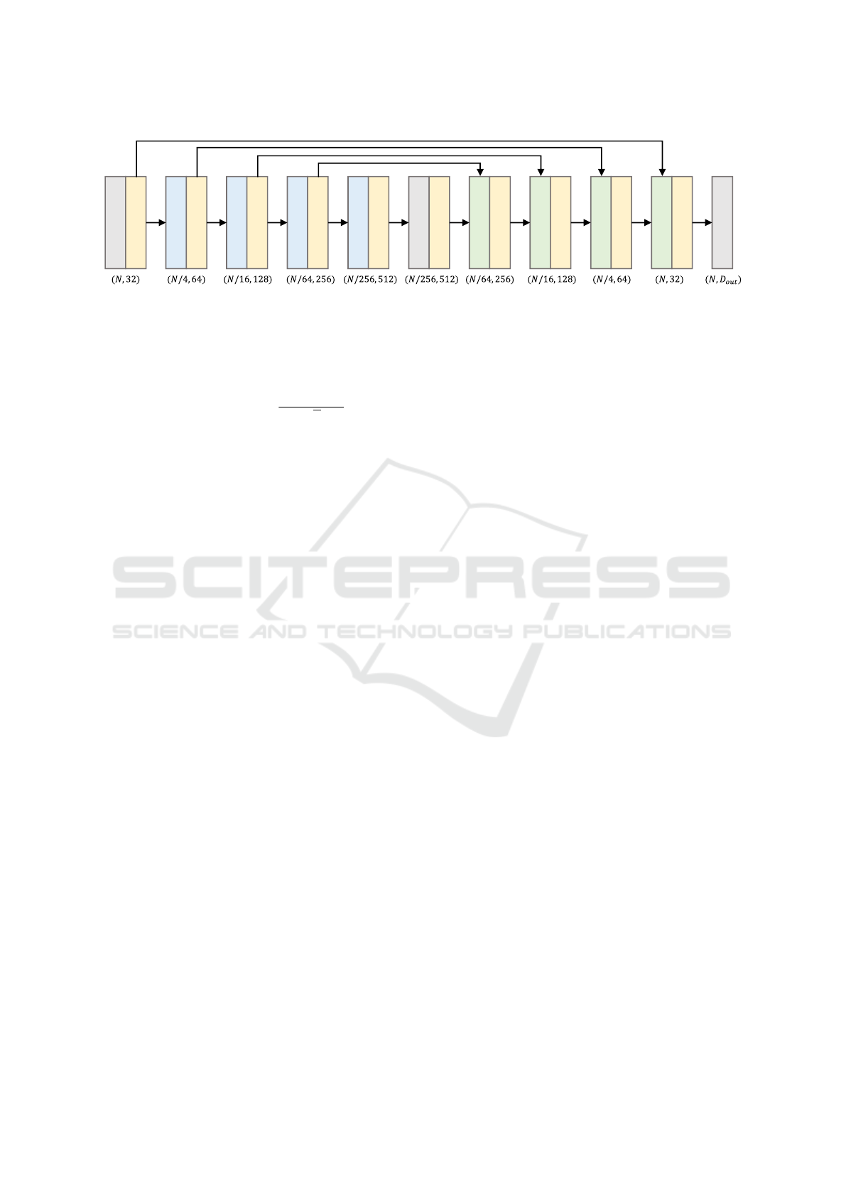
Figure 1: Overview of the Point Transformer architecture for semantic segmentation. Grey boxes are MLPs, blue boxes are

downsample blocks, yellow boxes are 1 to n Point Transformer blocks, and green boxes are upsample blocks. N is the number

of points followed by the feature length, D

out

is the number of classes. (adapted from(Zhao et al., 2020b)).

attention for a given feature x

and set of features X

can attend to, can be deﬁned as

sa(x

, X

) =

∑

∈X

so ftmax(

q(x

)

k(x

)

√

)v(x

Usually q, k, and v are linear projections or MLPs and

d is the output dimensionality of q and k. For VA this

computation is slightly different:

va(x

, X

) =

∑

∈X

so ftmax(w(q(x

) −k(x

))) ⊙v(x

In the Point Transformer, X

is speciﬁcally deﬁned as

the k nearest neighbors of x

, w is an MLP and ⊙is the

hadamard product (element-wise multiplication). So

in VA, the attention weights are vectors rather than

scalars, hence the name. This allows the operation

to modulate individual channels of the value vectors.

The authors of the original paper have shown this

form of attention to perform signiﬁcantly better than

scalar dot-product attention in the context of 3D point

clouds.

The authors further adapted VA by adding a

learned position encoding δ to the attention vector and

the values:

va(x

, X

) =

∑

∈X

so f tmax(w(q(x

) −k(x

) + δ)) ⊙(v(x

) + δ),

(1)

where δ is deﬁned as

δ = MLP(p

−p

), (2)

with p

and p

being the absolute coordinates of the

points with features x

and x

. In words: The posi-

tion encoding is a learned representation of the rela-

tive position between two points. The authors have

shown that adding the position encoding to the atten-

tion vectors, as well as to the values, improves perfor-

mance. Note that this position encoding is not related

to the positional encoding used in NLP-Transformers,

in which the positional encoding is used to establish

an order between the tokens.

3.1.2 Down- and Upsampling

As mentioned above, the architecture ﬁrst reduces and

then restores a point clouds density. The downsam-

pling is done with farthest point sampling (FPS). FPS

starts with a random point and then adds the farthest

away point to the subset. This is repeated n times,

now with the distance being calculated to every point

in the subset, and the point with the biggest minimum

distance is added. Then all point features are pooled

onto the subset: First for each point in the subset the k

nearest neighbors from the initial point cloud are de-

termined. Then the features of those points are com-

bined via max pooling.

The upsampling blocks restore the point cloud

density by mapping the features of the coarser rep-

resentation to the ﬁner representation via trilinear in-

terpolation.

3.2 Point Transformer V2

In 2022, the authors proposed an optimization of their

architecture (Wu et al., 2022) that made the architec-

ture both faster and more accurate.

3.2.1 Grouped Vector Attention

One major change was the introduction of grouped

vector attention (GVA). While in the original VA

(Equation 1) the weight encoding MLP w produced a

weight for each channel of the respective value vector,

in GVA w produces a weight for a group of channels

in the value vector. Figures 2a & 2b in the original

paper (Wu et al., 2022) illustrate the difference.

Weighting groups of channels in each value vec-

tor, instead of individual channels, forces the model to

learn more generalizable representations, while also

reducing the parameter count of the weight encoding

MLP, which makes it computationally cheaper.

Note that GVA is not only a generalized form of

VA, but also of the commonly used multi-head self-

Efﬁciency Optimization Strategies for Point Transformer Networks

attention (Vaswani et al., 2017), as shown in the orig-

inal paper.

3.2.2 Grid Pooling & Map Unpooling

The second major change was the introduction of grid

pooling and map unpooling.

Grid pooling replaces FPS in the Point Trans-

former V1. It works by partitioning the point cloud

with a regular grid. Then the points in the same grid

cells are fused: The coordinates of the points by cal-

culating their mean, their features by max pooling.

Grid pooling allows for replacing the unpooling by

interpolation with unpooling by mapping. By caching

which points were fused during grid pooling, the fea-

ture of each combined point can simply be mapped to

the points it originated from.

Further changes include the omission of the

bottleneck-MLP (Figure 1) and changes to hyperpa-

rameters, layer order and scaling. We will cover these

in the ablation study (Section 6).

4 CONCEPT

While the Point Transformer architecture is powerful,

it is also computationally expensive to run and espe-

cially to train. Also some components rely on custom

CUDA kernels. While these signiﬁcantly speed up the

given component, they do so by a ﬂat factor and not

by improving the runtime complexity. Also out-of-

framework code, like a custom CUDA kernel, is in-

herently more cumbersome to use and might discour-

age from further research. The following sections de-

scribe strategies that improve the efﬁciency and ease

of implementation of the Point Transformer architec-

ture while preserving its accuracy.

4.1 Uniform Point Cloud Sizes

A major architecture difference in our version of the

point transformer is that we enforce a uniform num-

ber of points for our training point clouds as well as

for their internal downsampled versions. The original

implementation allowed for point clouds of different

sizes within the same batch by concatenating them

and later separating them with stored offsets where

required. So a batch of point clouds had the shape

(sum(point cloud sizes), 3), and a second vector with

offsets was required, while our batches have the shape

(batch size, point cloud size, 3), and no offset vector.

Our version eliminates the overhead for separating

and merging point clouds and calculating offsets, and

is thus faster. Also it is more intuitive and easier to

implement. Our evaluation shows that uniform point

cloud sizes during training do not restrict the model

to point clouds of the same size during inference, as

long as the difference between training and inference

size is not extreme (Section 5.6).

If the model is trained on synthetic data, like in

our case, generating point clouds with a uniform size

is not an issue. If the model is trained on a given

dataset with non-uniform point cloud sizes, we pro-

pose sampling the point clouds to a uniform size via

FPS. While FPS is expensive (as will be explained

in Section 4.2.1), it is acceptable as a pre-processing

step (rather than part of the architecture), as those

only need to be performed once per point cloud in the

dataset rather than once per point cloud, per epoch,

and per downsampling block.

4.2 Pooling

4.2.1 Problems of FPS & Grid Pooling

Version 1 uses FPS to downsample point clouds. Even

with an efﬁcient implementation, FPS has quadratic

runtime relative to the number of points. However, an

even bigger problem is that it is not parallelizable, as

we always need the points 0 to n to determine point

n+1. This synergizes very poorly with modern GPUs

that rely heavily on parallel computing. Thus, FPS is

very slow, especially for large point clouds.

While grid pooling is parallelizable and thus con-

siderably faster, it is not compatible with our idea of

keeping uniform point cloud sizes across all stages

of the architecture. As the uniform grid used in grid

pooling does not adapt to the point cloud, the pooled

version of a large object will consist of more points

than the pooled version of a small object. Therefore

we cannot assure uniform point cloud sizes if we were

to use grid pooling.

4.2.2 K-D Tree Pooling

As an alternative that can assure uniform point cloud

sizes while still being parallelizable, we propose pool-

ing the point clouds with a balanced k-D Tree (the

k being the three spatial dimensions). First, we de-

termine the dimension with the largest absolute delta

and split the point cloud along this dimension into two

equally sized partitions. Then, this process is repeated

for all individual partitions until the partitions contain

a desired number of points. Lastly, we fuse the points

in each partition by taking their mean. Figure 2 visu-

alizes the process in 2D.

Similar to grid pooling we combine the point’s

features by max pooling across all points in a given

partition. As our pooling method also fuses sets of

VISAPP 2024 - 19th International Conference on Computer Vision Theory and Applications

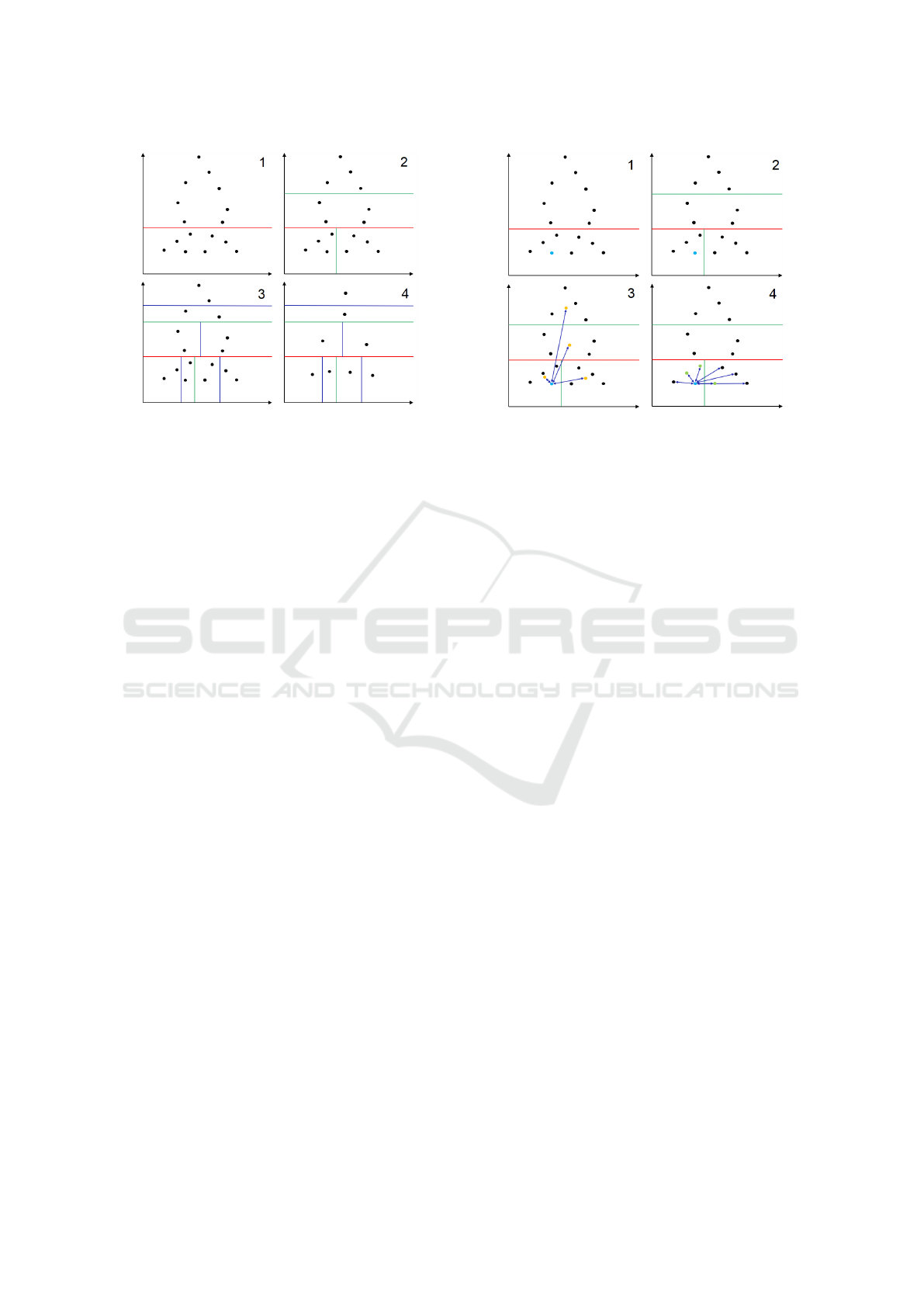
Figure 2: Illustration of k -D tree pooling in 2D. The ﬁrst

three images show the partitioning process (red, green, blue

lines). The last image shows the merging of points in the

same partition.

points to reduce the point cloud size (like grid pool-

ing, but unlike FPS), we can also use map unpooling

as described in Section 3.2.2 to restore the point cloud

sizes in the later half of our architecture.

4.3 K-D Tree K Nearest Neighbors

The original Point Transformer uses an algorithm

based on heap sort which is implemented as a custom

CUDA kernel to ﬁnd the k nearest neighbors (KNN)

of each point. We propose to instead use a k-D tree

based algorithm, as it allows us to reuse the partitions

from the KNN search during pooling.

First we partition the point cloud until each par-

tition reaches a deﬁned size, as described in the pre-

vious section, and calculate the mean of the points in

each partition. Then, if we want to ﬁnd the KNNs of

point i, we ﬁrst ﬁnd the n nearest partition means and

then search for the KNNs only in these n partitions.

The lower n is chosen, the faster the search is, but the

higher the chance becomes, that one of the KNNs is

outside the considered partitions and will thus not be

found. Figure 3 visualizes the process in 2D.

If the point clouds we want to process become

very large, we can end up with a large number of par-

titions and/or very big partitions. In this case, we can

perform the algorithm in multiple steps. By interpret-

ing the means of the points in each partition as a point

cloud itself, we can use the same algorithm to efﬁ-

ciently ﬁnd the KNNs in the new point cloud. This

approach can be stacked indeﬁnitely. Also it can be

implemented very efﬁciently as we can reuse the par-

titions from the initial point cloud for the partition-

mean-point cloud.

Figure 3: Illustration of k-D tree KNN search in 2D. In this

example, we search the k=4 nearest neighbors of the light

blue point. The ﬁrst two images show the k-D tree parti-

tioning process (red & green lines). As those are identi-

cal to the the partitions for the KNN search (the ﬁrst two

images in Figure 2), we can reuse them. The third image

shows the distance calculations (blue arrows) between the

light blue point and the partition means (yellow points). The

fourth image shows the distance calculations (blue arrows)

between the light blue point and the points in the n=2 near-

est partitions. The k=4 nearest neighbors include the light

blue point itself and the points highlighted in light green.

4.4 Normalizing the KNN Relative

Positions

During our comparison of different downsample al-

gorithms we found that, in general, algorithms that

produce a very consistent density in the downsam-

pled point cloud, regardless of the input point cloud,

perform best. This is in line with the ﬁndings of the

Point Transformer V2 paper that found grid pooling

to be superior to FPS. While FPS produces a very

well spread subset, it downsamples point clouds by

a ﬁxed factor. Therefore, point clouds of small ob-

jects remain denser than point clouds of large objects.

Grid pooling produces the same density, regardless of

object size. It increases or decreases the number of

points instead.

As our k-D tree pooling approach does not pro-

duce quite as well spread subsets as FPS, nor does it

change the number of output points to always produce

the same density like grid pooling, we propose to ex-

plicitly normalize the density. Globally normalizing

the density of a point cloud after each downsampling

stage is not possible without changing the number of

points in the downsampled point cloud, or without ex-

cessive computation. However, apart from the down-

sample algorithm itself, the point coordinates are only

ever used to compute the position encoding between a

point and its KNNs (Equation 2). We can therefore re-

Efﬁciency Optimization Strategies for Point Transformer Networks

formulate Equation 2 to normalize the local density.

We do so by adjusting the relative position between

point p

and each of its KNNs p

(the vectors from

to each p

), so that their Euclidean lengths have a

standard deviation of 1:

δ = MLP(normalize(∆p

i, j

)),

∆p

i, j

= p

−p

normalize(∆p

i, j

) =

∆p

i, j

σ + ε

σ =

∑

j=1

|∆p

i, j

k −1

∑

j=1

∆x

i, j

+ ∆y

i, j

+ ∆z

i, j

k −1

∑

j=1

∆x

i, j

+ ∆y

i, j

+ ∆z

i, j

k −1

where σ is the standard deviation, ε is a small con-

stant for numeric stability, k is the number of neigh-

bors we attend to, and ∆x

i, j

, ∆y

i, j

and ∆z

i, j

are differ-

ences of the points p

and p

on the x, y and z axes.

This is the standard normalization approach of sub-

tracting the mean and dividing by the standard devia-

tion, except that in our case we explicitly do not want

to normalize the relative positions ∆p

i, j

around their

mean, but around the point p

that searched for the

KNNs. The relative position between p

and itself is

always (0, 0, 0) so we can just omit subtracting the

mean in our normalization procedure.

5 EVALUATION

5.1 Implementation

We used Tensorﬂow 2.10.0 and Keras 2.10.0 with

CUDA 11.3.1 and cuDNN 8.2.1 to implement the

model. For all our experiments we used mixed pre-

cision, meaning calculations are performed in half

precision, which makes them faster and requires less

RAM, while weights are stored in single precision for

numeric stability. In addition, we compiled all func-

tions for point cloud partitioning, un-partitioning, and

the KNN search to Tensorﬂow graphs to improve their

efﬁciency. We trained all models on a single NVIDIA

RTX 3080 Ti GPU with 12GB of RAM.

5.2 Datasets

We trained and evaluated our models on synthetic

data. Each point cloud in our datasets is sampled

from a scene with a random number of random prim-

itives (box, sphere, cylinder, cone, torus), with ran-

dom sizes, at random positions, and with random ori-

entations. The primitives can be partially outside the

space we consider (-1 to 1 for all three axes), in which

case they are cut off. We collect only the point co-

ordinates and no other features like color or normals.

Each point is labeled according to the shape of the sur-

face it belongs to (not the primitive type) to avoid am-

biguity. We distinguish between ﬂat surfaces, spheri-

cal surfaces, cylindrical surfaces, conical surfaces and

toroidal surfaces. For example a cylinder consists of

two ﬂat surfaces and one cylindrical surface. We use

this dataset over more popular benchmarks as we plan

to apply our ﬁndings to primitive instance segmenta-

tion in future work.

We generated two of these datasets, which will

further be referred to as ”dataset S” and ”dataset L”.

Dataset S consists of ∼32k (2

) point clouds and

each point cloud of 4096 (2

) points. The set of

primitives is exclusively combined by union. Dataset

L also consists of ∼32k (2

) point clouds, however

each point cloud consists of ∼32k (2

) points. Fur-

ther the set of primitives has a wider range of possi-

ble primitive numbers and sizes and is combined by

union and difference, which allows for more complex

shapes that are therefore harder to semantically seg-

ment. The differences between datasets S and L are

summarized in Table 1 and visualized in Figure 4.

Table 1: Comparison of the datasets we used.

n n n Prim. Comb.

Clouds Points Prims Sizes Ops

S 2

4 to 10 0.3 to union

1.5

L 2

6 to 15 0.1 to union

2.5 & diff.

5.3 Description of the Baseline Point

Transformer

As a baseline we recreated the Point Transformer V1

because the grid pooling in V2 is inherently not com-

patible with our plan to use uniform point cloud size

in all stages of the model. The ofﬁcial implementation

of the Point Transformer V1 already includes GVA,

even though it was ﬁrst published in the follow-up pa-

per. As the ofﬁcial implementation includes GVA and

we want to ensure that our efﬁciency gains did not

VISAPP 2024 - 19th International Conference on Computer Vision Theory and Applications

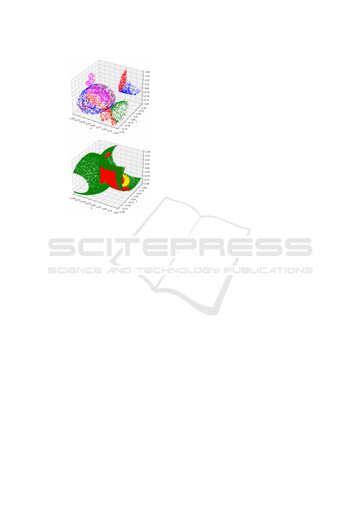
Figure 4: Visualization of a point cloud from dataset S (top)

and one from dataset L (bottom). Flat surfaces are red,

spherical surfaces are green, cylindrical surfaces are blue,

conical surfaces are yellow, and toroidal surfaces are pink.

solely come from GVA, we also included GVA in our

baseline model.

Further, during our experiments with different

downsampling algorithms, we found that starting FPS

with a random point (instead of always the ”ﬁrst”

point) during training improves generalization. This

intuitively makes sense as the inner stages now re-

ceive different point cloud subsets in each epoch,

which acts as regularization. This form of regular-

ization has the advantage over other regularization

techniques, like dropout or weight decay, that it does

not restrict the model in any way. Therefore it only

very mildly increases the number of epochs needed

to reach convergence (compared to e.g. dropout or

weight decay). The additional computation needed

for generating random starting points is negligible.

We included this improved FPS in our baseline model

to not skew the comparison in our favor by withhold-

ing simple optimizations.

Regarding the hyperparameters we use a single

Point Transformer block after the embedding-MLP,

each downsample block, the bottleneck-MLP, and

each upsample block. The ﬁve stages in our model

use the feature lengths from Point Transformer V1

(32, 64, 128, 256, 512). Each stage reduces the num-

ber of points in a cloud by factor 4. In the following

sections we refer to this conﬁguration as ”small”. Fur-

ther we use group size 8 and attend to the 16 nearest

neighbors in all GVA layers.

If not explicitly stated otherwise, we use our k-D

tree based KNN search algorithm (Section 4.3) in all

our models. To keep the code simple, we never use

the multi-stage variant of the algorithm, even though

it would probably speed up the computation measur-

ably (especially on the larger point clouds in dataset

L). We search in 8 partitions with 16 (dataset S) or

32 (dataset L) points each. These values are not arbi-

trary: As we always split our point clouds along the

axis with the largest delta, we usually start to cycle

through the three axes after the ﬁrst few splits. This

results in the later partitions creating a roughly uni-

form grid. The worst case for ﬁnding the KNNs of

a point is if that point is in a corner of its partition.

However, under the assumption of a uniform grid and

each partition containing at least k points, we are en-

sured to discover all KNNs by searching within the

partition containing the point and the seven partitions

surrounding the corner where the point is located.

5.4 Description of the Adapted Point

Transformer

Our version of the Point Transformer builds on the

baseline model described above. Further we adopt the

map unpooling and the omission of the bottleneck-

MLP from V2, and introduce our k-D tree pooling and

KNN normalization strategy. We also included 0.1

dropout directly after the softmax calculation in GVA

during training on dataset S.

In addition to the ”small” conﬁguration we also

trained a model with a ”medium” and a ”large”

conﬁguration. The small conﬁguration remains un-

changed, the medium conﬁguration uses two instead

of one Point Transformer block after each downsam-

ple block, and the large conﬁguration uses (2, 2, 6,

2) Point Transformer blocks after the downsample

blocks and feature lengths (48, 96, 192, 384, 512) in

the ﬁve stages of the model. The large conﬁguration

was also used in the Point Transformer V2 paper.

Note that when excluding the bottleneck-MLP we

also excluded the Point Transformer block immedi-

ately succeeding it. Therefore the small conﬁguration

of our model has one Point Transformer block less

than the small baseline model.

5.5 Comparisons

5.5.1 Dataset S

For dataset S we trained all our models in three stages

with learning rates 0.005, 0.001, and 0.0002. For all

Efﬁciency Optimization Strategies for Point Transformer Networks

stages we used an Adam optimizer (Kingma and Ba,

2017), early stopping with patience 6, and a hard cap

of 50 epochs per stage. If early stopping triggered

or the hard cap was reached, we rolled the weights

back to the epoch with the best validation loss and

proceeded with the next stage. Table 2 shows the re-

sults.

Table 2: Comparison of the baseline model and our archi-

tecture on a dataset S.

Arch. Param. BS RAM Acc. Epoch

(M) (GB) (%) Time

Baseline 4.9 48 7.0 97.0 883s

(small)

Ours 2.7 48 6.7 96.6 404s

(small)

Ours 4.5 48 7.7 97.4 462s

(med.)

Ours 9.5 8 6.7 97.5 1682s

(large)

Our small model performed slightly worse than

the small baseline model. However, this is in part

due to the huge parameter disparity. Comparing the

baseline model to our medium model, which still has

less parameters, our model performs slightly better,

while still being almost twice as fast. Using the large

conﬁguration only resulted in minor improvements in

accuracy, while memory requirements increased dras-

tically, forcing us to use a smaller batch size (BS),

which slowed down training signiﬁcantly. Further,

comparing the training histories, our models are much

more stable and overﬁt less. The improved stability is

a direct result of introducing our normalization of the

KNN’s relative positions.

5.5.2 Dataset L

For training on dataset L we used the same setup as

on dataset S, with the exception that we lowered the

early stopping patience to 2 to save time. Judging

by our training history, a larger patience could prob-

ably improve our accuracy. Table 3 shows our re-

sults. We trained our medium-sized model until con-

vergence because, even with a more aggressive pa-

tience, training on this larger dataset takes approxi-

mately 30 hours with our medium model.

Comparing the training speed of the baseline

model with ours on dataset S and L, one can see the

importance of an efﬁcient downsampling algorithm

increasing with the size of the point clouds. Further,

we hypothesize that with larger point clouds the cho-

sen sampling method becomes less relevant in terms

of accuracy, since preserving a point cloud’s recogniz-

able shape becomes easier the more points one uses.

Table 3: Comparison of the baseline model and our archi-

tecture on dataset L. The ”Epoch Time” for the baseline

model is an estimation based on 10% of the dataset.

Arch. Param. BS RAM Acc. Epoch

(M) (GB) (%) Time

Baseline 4.9 8 6.3 - ∼16h

(small)

Ours 2.7 8 5.8 - 44m

(small)

Ours 4.5 8 8.9 97.4 50m

(med)

However, given the time training our baseline model

on dataset L would take, we could not test our hypoth-

esis.

5.5.3 Analysis of Efﬁciency Bottlenecks

In an effort to identify efﬁciency bottlenecks in our ar-

chitecture we measured the timing of individual com-

ponents of our model. We speciﬁcally focused on

the algorithmic parts of the model (those without any

learnable parameters), as those make up a signiﬁcant

part of the computational cost and provide the most

direct opportunities for optimization. Table 4 shows

how much of a data batch’s processing time goes into

the KNN search, the downsampling algorithm, and

the upsampling algorithm, given different point cloud

sizes and model conﬁgurations. We also included a

version of our baseline model that uses a brute force

search to ﬁnd the KNNs. Lastly we calculated the

”remaining time” that was actually spent on calcula-

tions with learnable weights, normalizations and non-

linearities.

Table 4 highlights the importance of an efﬁ-

cient KNN search algorithm, especially for process-

ing large point clouds. This is also evident in the up-

sampling time of the baseline models, as they need

to ﬁnd the k = 3 nearest neighbors to calculate the

trilinear interpolations. Moreover, the synergy be-

tween our k-d tree based KNN search and our k-d

tree based pooling is evident in the very fast down-

sampling times. As we already partitioned our point

clouds into sets of 16 (or 32 in case of the size 32768

point clouds) during the KNN search, our downsam-

pling merely consists of splitting those partitions an-

other 2 (3) times and calculating the partition centers.

On the contrary, FPS, the downsampling algorithm

used in the baseline model, accounts for over 90% of

the processing time for larger point clouds (given that

the efﬁcient KNN search algorithm is used), which

makes it non-viable in this context. Our normaliza-

tion of the KNN relative positions took less than 5ms.

VISAPP 2024 - 19th International Conference on Computer Vision Theory and Applications

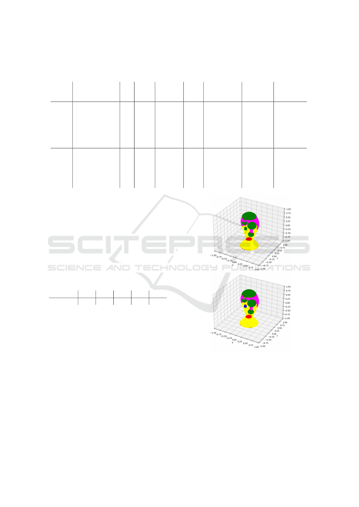
Table 4: Speed comparison of a version of the baseline model that uses a brute force approach to search the KNNs, the usual

baseline model and our architecture. The experiments were performed in eager mode, which is required to accurately time

individual components of a model, but is overall slower.

n Architecture BS RAM Time per KNN Downsample Upsample Remaining

Points (GB) Batch Time Time (ms) Time (ms) Time (ms)

(ms) (ms)

4096 Baseline with 64 8.2 1890 555 566 427 342

brute force KNN

search (small)

4096 Baseline (small) 64 8.2 1695 361 587 400 347

4096 Ours (small) 64 8.0 927 365 46 183 333

4096 Ours (medium) 64 8.8 976 363 45 182 386

4096 Ours (large) 8 6.6 774 186 29 113 446

32768 Baseline with 8 6.6 20071 6237 12567 941 326

brute force KNN

search (small)

32768 Baseline (small) 8 6.5 13677 394 12531 415 337

32768 Ours (small) 8 6.3 847 384 48 104 311

32768 Ours (medium) 8 7.4 955 389 51 112 403

5.6 Analysis of Different Training and

Inference Point Cloud Sizes

As mentioned in Section 4.1 we experimented with

using point clouds of different sizes during inference

to conﬁrm that using uniform point cloud sizes during

training does not limit the model to that speciﬁc size

during inference.

Table 5: Comparison of different point cloud sizes dur-

ing inference with our medium model trained on dataset L

(which contains point clouds of size ∼32k (2

)). The re-

ported accuracies are the averages of 4096 point clouds.

n Points 2

Acc. (%) 91.6 97.7 97.4 95.9 92.0

Table 5 shows that using slightly bigger point

clouds during inference even improves accuracy. This

is analogous to image processing, where training on

smaller images than the ones used during inference is

a known method to increase training speed while pre-

serving or even slightly improving accuracy (Howard

and Gugger, 2020). This makes intuitively sense: For

any given point our model attends to a ﬁxed num-

ber of neighbors (16 in our case). If we double the

total number of points in the point cloud, the effec-

tive ”ﬁeld of view” of any point becomes half as big,

which we can reinterpret as all objects in the point

cloud becoming twice as big. This enlargement helps

with correctly labeling very small objects, which is

usually very difﬁcult (Figure 5). This reinterpretation

is strengthened even further in our model as we effec-

tively eliminate the absolute scale in any local region

with our normalization of the KNN relative positions.

Figure 5: Zero-shot results of our medium model trained

with dataset L on point clouds from the ABC-dataset (Koch

et al., 2019). The upper cloud consists of ∼64k (2

) points,

the lower cloud consists of ∼32k (2

) points. Red points

were classiﬁed as ﬂat surfaces, green ones as spherical sur-

faces, blue ones as cylindrical surfaces, yellow ones as coni-

cal surfaces, and pink ones as toroidal surfaces. In the lower

cloud with ∼32k points the model incorrectly classiﬁed the

surfaces of the small bubbles as cylindrical and a small part

as ﬂat, while it correctly labeled them as spherical in the

upper cloud with ∼64k points.

However, ”zooming further and further in” makes any

surface eventually appear ﬂat, which then leads to a

Efﬁciency Optimization Strategies for Point Transformer Networks

decline in accuracy. In contrast, reducing the size and

thereby the detail of a point cloud gradually reduces

the accuracy, which is also intuitive. Nevertheless, up

to a certain point, the accuracy decline remains ac-

ceptable (-1.49% accuracy during inference with half

the training size).

6 ABLATION STUDY

During our ablation study we used more aggressive

learning rates of 0.01, 0.001, and 0.0001, and reduced

the early stopping patience to 2. This leads to an over-

all worse accuracy, but also to faster convergence. All

other training conﬁgurations are identical to the ones

used in the evaluation.

6.1 Ablation of Novel Optimizations &

Changes Adopted from Point

Transformer Version 2

Table 6 shows the incremental changes we made to

the Point Transformer. As a starting point, we uti-

lized the small conﬁguration of version 1 because grid

pooling in version 2 is inherently incompatible with

maintaining consistent point cloud sizes. All changes

will be discussed in the following sections:

1. While introducing GVA sped up training and re-

duced RAM usage, even with a larger batch size,

it also reduced our accuracy. However this is to be

expected, as we train a rather small model (4.87M

parameters) on a comparably big dataset (∼134M

) points in total). So adding more parameters

in any form usually helps. Another way to look

at it is that GVA is a way to regularize regular

VA. Regularization usually only improves perfor-

mance if overﬁtting is an issue (which it is not in

this case, given we train a small model on a large

dataset) and degrades the performance otherwise.

However, the original paper shows GVA signiﬁ-

cantly outperforming regular VA in larger models,

which we will eventually move to, so we adopted

the change.

2. Next, we replaced FPS with our k -D tree based

approach. While this further reduced accuracy,

it signiﬁcantly sped up training, which becomes

imperative when training on bigger point clouds

as shown in Section 5.5.2. As mentioned in that

section, we expect the accuracy difference to de-

crease with bigger point clouds.

3. Unpooling via mapping instead of interpolation

is faster and more accurate, at the minor cost of

slightly more RAM usage for storing the point in-

dices during pooling so they can later be mapped

back. Overall, this change is very positive.

4. Using a combination of dropout and GVA for reg-

ularization achieves higher accuracies than just in-

creasing the group size of the GVA. Especially

in smaller model conﬁgurations, increasing the

group size, and thereby reducing the parameter

count, is counterproductive as mentioned in point

1, and dropout becomes a more viable alternative.

5. Removing the bottleneck-MLP and the succeed-

ing Point Transformer block reduced the accuracy,

although considering the big parameter count dis-

parity to the prior version, not by much. Follow-

ing the original Point Transformer V2 we omit the

bottleneck.

6. Next, we added an additional Point Transformer

block after every downsampling block to make up

the parameter difference, leading to our medium

conﬁguration. Increasing the model depth made

it signiﬁcantly more accurate, but also slightly

slower. Also, as we kept the rather high learn-

ing rate and the low patience, training the deeper

model became unstable, leading to accuracies de-

viating as much as 0.52% from the reported mean.

7. Lastly, we added our normalization of the KNN

relative positions. While not measurably slowing

down training, it signiﬁcantly improved the accu-

racy and training stability, even when compared

to the slower baseline model. However, similar to

GVA, it appears to become effective only with a

certain model size. During our tests, normalizing

the KNN relative positions in small models actu-

ally degraded their performance.

6.2 Analysis of Point Transformer V2’s

Changes to Layer Order & Scaling

Point Transformer V2 changed two implementation

details: Firstly, while version 1 calculated queries and

keys with a simple dense layer and the weight encod-

ing MLP had the structure: batch norm, ReLU, dense,

batch norm, ReLU, dense, version 2 calculates the

queries and keys via dense, batch norm, ReLU, and

the weight encoding MLP consists of: dense, batch

norm, ReLU, dense. Secondly, the position encoding

MLP’s hidden size is increased from a constant 3 to

always match the current feature dimension. How-

ever, in our experiments, both modiﬁcations led to a

decrease in the model’s accuracy and speed. As a re-

sult, we opted not to adopt these changes (Table 7).

VISAPP 2024 - 19th International Conference on Computer Vision Theory and Applications

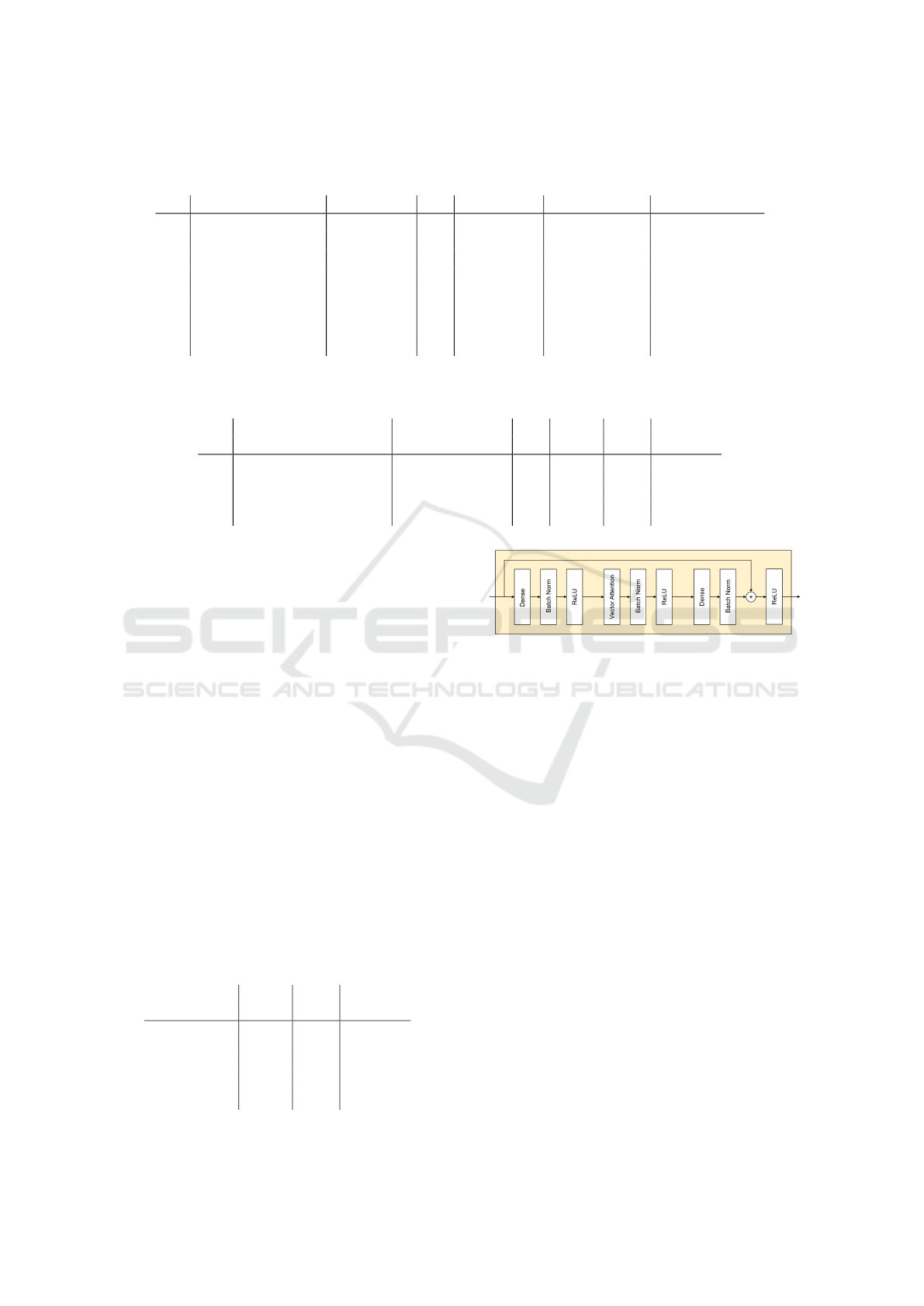
Table 6: Incremental changes from the Point Transformer V1 (small) to our architecture. All numbers refer to training on

dataset S. While repeating our experiments the accuracies in the second to last step varied greatly, so we report an average.

ID Changes Param. (M) BS RAM (GB) Acc. (%) Epoch Time (s)

0 PTv1 6.18 48 9.0 97.09 928

1 +GVA (= baseline) 4.87 64 8.5 96.43 802

2 +k-D Tree Pooling 4.87 64 8.0 94.30 526

3 +Map Unpooling 4.87 64 8.1 95.28 489

4 +Dropout 4.87 64 8.2 95.90 494

5 -Bottleneck 2.72 64 8.0 95.52 488

6 +More PT Blocks 4.54 64 9.3 96.51 (±0.52) 531

7 +knn norm 4.54 64 9.3 97.32 529

Table 7: Analysis of the changes to Layer Order & Scaling in the attention calculation Point Transformer V2 introduced. All

experiments used a medium conﬁguration and dataset S.

ID BN and ReLU directly Bigger Position- BS RAM Acc. Epoch

on Query & Key Encoding MLP (GB) (%) Time (s)

1 64 9.3 96.8 533

2 ✓ 64 7.9 95.9 542

3 ✓ 48 9.4 96.6 569

4 ✓ ✓ 48 8.5 95.0 591

6.3 Analysis of ”More Standard”

Transformer Block Structures

Given that the Transformer block structure used in the

Point Transformer (Figure 6) is unusual, we compared

it with a more standard Transformer block struc-

ture (attention, normalization and a skip connection

around them followed by an MLP, normalization and

another skip connection around them) which is used

in most transformer models. We also compared the

original Point Transformer with a version that uses

layer normalization (Ba et al., 2016) instead of batch

normalization (Ioffe and Szegedy, 2015), as this is

also the more common choice in transformer archi-

tectures (Vaswani et al., 2017; Brown et al., 2020;

Liu et al., 2021; Yang et al., 2023; Lai et al., 2022).

However, both changes signiﬁcantly degraded perfor-

mance, so we did not investigate them further (Table

8).

Table 8: Comparison of the baseline model, a version with

the standard Transformer block structure, and a version with

layer norm instead of batch norm. All experiments were

performed on a very small, earlier version of our dataset.

Arch. RAM Acc. Epoch

(GB) (%) Time (s)

Baseline 6.4 95.2 39

(small)

Std. Block 6.4 92.9 39

Structure

Layer Norm 7.5 91.9 43

Figure 6: Structure of the Point Transformer block.

7 CONCLUSION

We proposed a variant of the Point Transformer ar-

chitecture that is considerably more efﬁcient for pro-

cessing large point clouds. At similar model sizes,

we reached more than 19 times faster training times.

While we were unable to directly compare the result-

ing accuracies on those larger point clouds due to the

extreme computational cost of the original architec-

ture, the observed disparity does not seem signiﬁcant.

Further, we posit that the accuracy loss resulting from

our simpler downsampling approach should dimin-

ish with the size of the point cloud, while the better

runtime complexity of our architecture becomes more

important.

Further research might include testing our ar-

chitecture on more datasets, like the S3DIS- (Ar-

meni et al., 2017) or the SemanticKITTI (Behley

et al., 2019) dataset. Particularly, datasets with non-

uniform densities owing to perspective, such as Se-

manticKITTI, could be of interest. Our downsam-

pling approach does not homogenize these densities,

potentially enabling our model to be more precise in

Efﬁciency Optimization Strategies for Point Transformer Networks

regions near the LiDAR sensor where the point cloud

is denser and, consequently, more detailed.

REFERENCES

Armeni, I., Sax, A., Zamir, A. R., and Savarese, S. (2017).

Joint 2D-3D-Semantic Data for Indoor Scene Under-

standing. ArXiv e-prints.

Ba, J. L., Kiros, J. R., and Hinton, G. E. (2016). Layer

normalization.

Behley, J., Garbade, M., Milioto, A., Quenzel, J., Behnke,

S., Stachniss, C., and Gall, J. (2019). SemanticKITTI:

A Dataset for Semantic Scene Understanding of Li-

DAR Sequences. In Proc. of the IEEE/CVF Interna-

tional Conf. on Computer Vision (ICCV).

Brown, T. B., Mann, B., Ryder, N., Subbiah, M., Kaplan, J.,

Dhariwal, P., Neelakantan, A., Shyam, P., Sastry, G.,

Askell, A., Agarwal, S., Herbert-Voss, A., Krueger,

G., Henighan, T., Child, R., Ramesh, A., Ziegler,

D. M., Wu, J., Winter, C., Hesse, C., Chen, M., Sigler,

E., Litwin, M., Gray, S., Chess, B., Clark, J., Berner,

C., McCandlish, S., Radford, A., Sutskever, I., and

Amodei, D. (2020). Language models are few-shot

learners. CoRR, abs/2005.14165.

Chen, X., Ma, H., Wan, J., Li, B., and Xia, T. (2016). Multi-

view 3d object detection network for autonomous

driving. CoRR, abs/1611.07759.

Choy, C. B., Gwak, J., and Savarese, S. (2019). 4d spatio-

temporal convnets: Minkowski convolutional neural

networks. CoRR, abs/1904.08755.

Dosovitskiy, A., Beyer, L., Kolesnikov, A., Weissenborn,

D., Zhai, X., Unterthiner, T., Dehghani, M., Min-

derer, M., Heigold, G., Gelly, S., Uszkoreit, J., and

Houlsby, N. (2020). An image is worth 16x16 words:

Transformers for image recognition at scale. CoRR,

abs/2010.11929.

Graham, B., Engelcke, M., and van der Maaten, L. (2017).

3d semantic segmentation with submanifold sparse

convolutional networks. CoRR, abs/1711.10275.

Guo, M., Cai, J., Liu, Z., Mu, T., Martin, R. R., and Hu,

S. (2020). PCT: point cloud transformer. CoRR,

abs/2012.09688.

He, K., Zhang, X., Ren, S., and Sun, J. (2015). Deep

residual learning for image recognition. CoRR,

abs/1512.03385.

Howard, J. and Gugger, S. (2020). Deep Learning for

Coders with Fastai and Pytorch: AI Applications

Without a PhD. O’Reilly Media, Incorporated.

Ioffe, S. and Szegedy, C. (2015). Batch normalization: Ac-

celerating deep network training by reducing internal

covariate shift. CoRR, abs/1502.03167.

Kingma, D. P. and Ba, J. (2017). Adam: A method for

stochastic optimization.

Koch, S., Matveev, A., Jiang, Z., Williams, F., Artemov, A.,

Burnaev, E., Alexa, M., Zorin, D., and Panozzo, D.

(2019). Abc: A big cad model dataset for geometric

deep learning. In The IEEE Conference on Computer

Vision and Pattern Recognition (CVPR).

Lai, X., Liu, J., Jiang, L., Wang, L., Zhao, H., Liu, S., Qi,

X., and Jia, J. (2022). Stratiﬁed transformer for 3d

point cloud segmentation.

Lecun, Y., Bottou, L., Bengio, Y., and Haffner, P. (1998).

Gradient-based learning applied to document recogni-

tion. Proceedings of the IEEE, 86(11):2278–2324.

Liu, Z., Lin, Y., Cao, Y., Hu, H., Wei, Y., Zhang, Z., Lin,

S., and Guo, B. (2021). Swin transformer: Hierarchi-

cal vision transformer using shifted windows. CoRR,

abs/2103.14030.

Maturana, D. and Scherer, S. (2015). Voxnet: A 3d convolu-

tional neural network for real-time object recognition.

In 2015 IEEE/RSJ International Conference on Intel-

ligent Robots and Systems (IROS), pages 922–928.

Qi, C. R., Su, H., Mo, K., and Guibas, L. J. (2016). Pointnet:

Deep learning on point sets for 3d classiﬁcation and

segmentation. CoRR, abs/1612.00593.

Qi, C. R., Yi, L., Su, H., and Guibas, L. J. (2017). Point-

net++: Deep hierarchical feature learning on point sets

in a metric space. CoRR, abs/1706.02413.

Robert, D., Raguet, H., and Landrieu, L. (2023). Efﬁ-

cient 3d semantic segmentation with superpoint trans-

former.

Su, H., Maji, S., Kalogerakis, E., and Learned-Miller, E. G.

(2015). Multi-view convolutional neural networks for

3d shape recognition. CoRR, abs/1505.00880.

Vaswani, A., Shazeer, N., Parmar, N., Uszkoreit, J.,

Jones, L., Gomez, A. N., Kaiser, L., and Polo-

sukhin, I. (2017). Attention is all you need. CoRR,

abs/1706.03762.

Wang, Y., Sun, Y., Liu, Z., Sarma, S. E., Bronstein, M. M.,

and Solomon, J. M. (2018). Dynamic graph CNN for

learning on point clouds. CoRR, abs/1801.07829.

Wu, X., Lao, Y., Jiang, L., Liu, X., and Zhao, H. (2022).

Point transformer v2: Grouped vector attention and

partition-based pooling.

Yang, Y.-Q., Guo, Y.-X., Xiong, J.-Y., Liu, Y., Pan, H.,

Wang, P.-S., Tong, X., and Guo, B. (2023). Swin3d: A

pretrained transformer backbone for 3d indoor scene

understanding.

Zhao, H., Jia, J., and Koltun, V. (2020a). Explor-

ing self-attention for image recognition. CoRR,

abs/2004.13621.

Zhao, H., Jiang, L., Jia, J., Torr, P. H. S., and Koltun, V.

(2020b). Point transformer. CoRR, abs/2012.09164.

VISAPP 2024 - 19th International Conference on Computer Vision Theory and Applications