CaRe-CNN: Cascading Reﬁnement CNN for Myocardial Infarct

Segmentation with Microvascular Obstructions

Franz Thaler

1,2 a

, Matthias A. F. Gsell

1 b

, Gernot Plank

1 c

and Martin Urschler

3 d

Gottfried Schatz Research Center: Medical Physics and Biophysics, Medical University of Graz, Graz, Austria

Institute of Computer Graphics and Vision, Graz University of Technology, Graz, Austria

Institute for Medical Informatics, Statistics and Documentation, Medical University of Graz, Graz, Austria

Keywords:

Machine Learning, Image Segmentation, Myocardial Infarction.

Abstract:

Late gadolinium enhanced (LGE) magnetic resonance (MR) imaging is widely established to assess the vi-

ability of myocardial tissue of patients after acute myocardial infarction (MI). We propose the Cascading

Reﬁnement CNN (CaRe-CNN), which is a fully 3D, end-to-end trained, 3-stage CNN cascade that exploits

the hierarchical structure of such labeled cardiac data. Throughout the three stages of the cascade, the label

deﬁnition changes and CaRe-CNN learns to gradually reﬁne its intermediate predictions accordingly. Further-

more, to obtain more consistent qualitative predictions, we propose a series of post-processing steps that take

anatomical constraints into account. Our CaRe-CNN was submitted to the FIMH 2023 MYOSAIQ challenge,

where it ranked second out of 18 participating teams. CaRe-CNN showed great improvements most notably

when segmenting the difﬁcult but clinically most relevant myocardial infarct tissue (MIT) as well as microvas-

cular obstructions (MVO). When computing the average scores over all labels, our method obtained the best

score in eight out of ten metrics. Thus, accurate cardiac segmentation after acute MI via our CaRe-CNN allows

generating patient-speciﬁc models of the heart serving as an important step towards personalized medicine.

1 INTRODUCTION

Cardiovascular diseases are the leading cause of death

worldwide among which myocardial infarction (MI)

is one of the most prevalent diseases

. MI is caused by

a decrease or complete cessation of blood ﬂow in the

coronary arteries which reduces perfusion in the sup-

plied myocardial tissue, leading to a metabolic under-

supply that impairs cardiac function and, ultimately,

may result in myocardial necrosis. The accurate as-

sessment of tissue damage after acute MI is highly

relevant as the extension of myocardial necrosis is an

important risk factor for developing heart failure. On

one hand, viable myocardial tissue with a potential

for functional recovery on restoration of normal blood

supply by revascularization might recover (Wrob-

lewski et al., 1990; Perin et al., 2002), which may

improve the functional capacity and survival (Van der

Wall et al., 1996; Kim and Manning, 2004). On the

other hand, precise delineation of infarcted myocar-

https://orcid.org/0000-0002-6589-6560

https://orcid.org/0000-0001-7742-8193

https://orcid.org/0000-0002-7380-6908

https://orcid.org/0000-0001-5792-3971

https://www.who.int/health-topics/cardiovascular-

diseases, last accessed on October 8, 2023

dial tissue is crucial to determine the risk of further

adverse cardiovascular events like ventricular tachy-

cardia which may lead to sudden death (Rosenthal

et al., 1985; Hellermann et al., 2002). For example,

the presence of microvascular obstructions, charac-

terized by a damaged microvasculature resulting in a

’no-reﬂow’ phenomenon preventing blood ﬂow from

penetrating beyond the myocardial capillary bed, is

linked to adverse ventricular remodeling and an in-

creased risk of future cardiovascular events (Hami-

rani et al., 2014; Rios-Navarro et al., 2019). Thus,

the accurate assessment of post-MI tissue damage is

of pivotal importance. In clinical practice magnetic

resonance (MR) imaging is used to quantify areas of

impaired myocardial function e.g. by estimating the

end-diastolic wall thickness of the left ventricle, or

by evaluating the contractile reserve, i.e. the myocar-

dial stress-to-rest ratio (Kim et al., 1999; Schinkel

et al., 2007). One of the most accurate methods is

late gadolinium enhanced (LGE) MR imaging, where

the contrast agent accumulates in impaired tissue ar-

eas, thus allowing to visualize the transmural extent of

tissues affected by MI (Selvanayagam et al., 2004).

However, analyzing LGE MR images to char-

acterize tissue viability in an accurate and efﬁcient

manner remains a signiﬁcant challenge. Nowadays,

Thaler, F., Gsell, M., Plank, G. and Urschler, M.

CaRe-CNN: Cascading Reﬁnement CNN for Myocardial Infarct Segmentation with Microvascular Obstructions.

DOI: 10.5220/0012324800003660

Paper published under CC license (CC BY-NC-ND 4.0)

In Proceedings of the 19th International Joint Conference on Computer Vision, Imaging and Computer Graphics Theory and Applications (VISIGRAPP 2024) - Volume 3: VISAPP, pages

53-64

ISBN: 978-989-758-679-8; ISSN: 2184-4321

Stage 1 Stage 2 Stage 3

Image x Image x Image x

Label y

Label Pred. y

Pred. p

Label Pred. y

Pred. p

M1, M12

convolution-dropout-convolution

pooling

upsampling

2x convolution

ﬁnal convolution

skip-connection

concatenation

Generalized Dice Loss

backpropagation

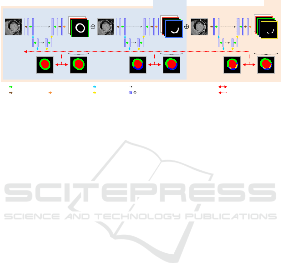
Figure 1: Overview of the proposed CaRe-CNN architecture for segmenting cardiac LGE MR images after MI. CaRe-CNN

is a 3-stage CNN cascade that exploits the hierarchical label deﬁnition of the data and reﬁnes intermediate predictions in

consecutive stages. The whole architecture is trained end-to-end and all data is processed in 3D. As MVO can only be present

for data of the D8 subgroup, we consider Stage 2 predictions as ﬁnal predictions for data of the M1 and M12 subgroups.

deep learning-based Convolutional Neural Networks

(CNNs) are widely adopted to medical image analy-

sis tasks like the detection of diseases in medical im-

ages (Esteva et al., 2017; Feng et al., 2022), or im-

age segmentation of the brain (Akkus et al., 2017),

the vertebrae (Payer et al., 2020), or the heart (Chen

et al., 2020). From cardiac LGE MR data, healthy and

necrotic myocardial tissue can be assessed by CNN-

based medical image segmentation, where each voxel

of an LGE MR image is assigned the respective label.

Accurate cardiac segmentation of patients after MI

can provide a foundation for generating anatomically

accurate patient-speciﬁc models of the heart, which,

in turn, can be used e.g., to create cardiac digital twin

models of human electrophysiology (Gillette et al.,

2021) to identify potential patient-speciﬁc causes for

arrhythmia improving personalized therapy planing

(Campos et al., 2022).

Due to the challenging nature of fully automated

infarct segmentation, some approaches in the liter-

ature rely on manual segmentations of the full my-

ocardium such that a distinction between healthy and

infarcted tissue only needs to be learned within that

region (Zabihollahy et al., 2018; Moccia et al., 2019).

Instead of using LGE MR data, (Xu et al., 2018)

uses cine MR data without contrast agents and a

Long Short-Term Memory-based Recurrent Neural

Network (Graves et al., 2013) to predict myocardial

infarct tissue from motion. In contrast to that, (Fahmy

et al., 2018) automatically segment both, healthy and

infarcted tissue from LGE MR images by employing

a 2D CNN based on the U-Net (Ronneberger et al.,

2015) architecture. In another fully-automated seg-

mentation approach, (Chen et al., 2022) employed

two consecutive 2D U-Net-like CNNs as a cascade,

where the ﬁrst network learns to segment the full

myocardium, while the second is trained to reﬁne

the prediction to obtain the infarct region. The au-

thors show that the consecutive setup achieves bet-

ter Dice and Jaccard scores, but worse volume esti-

mation compared to a parallel setup of two CNNs.

The semi-supervised myocardial infarction segmen-

tation approach in (Xu et al., 2022) proposes to use

attention mechanisms to obtain the coarse location of

the myocardial infarction before reﬁning the predic-

tion step-by-step. In order to allow training from un-

labeled data, they use an adversarial learning model

that provides a training objective even when ground

truth labels are not available. The EMIDEC chal-

lenge held in conjunction with the International Con-

ference on Medical Image Computing and Computer-

Assisted Intervention (MICCAI) in 2020 aimed to au-

tomatically segment myocardial infarct regions from

LGE MR images in their segmentation track (Lalande

et al., 2022). Different one- and two-stage approaches

mostly based on U-Net-like architectures were sub-

mitted by the challenge participants. The highest

scores in the segmentation track were achieved by

(Zhang, 2021) who employed a coarse to ﬁne two-

stage approach, where initial predictions are obtained

from a 2D U-Net variant before all 2D predictions are

stacked to a 3D volume. The stacked prediction in

combination with the LGE MR image is then reﬁned

by a 3D U-Net variant to obtain the ﬁnal prediction.

In this work, we propose the Cascading Reﬁne-

ment CNN (CaRe-CNN), which – differently to re-

lated work – is a fully 3D, end-to-end trained 3-stage

CNN cascade that exploits the hierarchical structure

of cardiac LGE MR images after MI and sequen-

tially reﬁnes the predicted segmentations. Further,

we propose a series of post-processing steps that take

anatomical constraints into account to obtain more

VISAPP 2024 - 19th International Conference on Computer Vision Theory and Applications

consistent qualitative predictions. Our CaRe-CNN

was submitted to the Myocardial Segmentation with

Automated Infarct Quantiﬁcation (MYOSAIQ) chal-

lenge which was held in conjunction with the Interna-

tional Conference on Functional Imaging and Mod-

eling of the Heart (FIMH) 2023. We evaluate our

method by comparing to state-of-the-art methods sub-

mitted to the MYOSAIQ challenge where our CaRe-

CNN ranked second out of 18 participating teams.

2 METHOD

In this work we propose CaRe-CNN, a cascading re-

ﬁnement CNN to semantically segment different car-

diac structures after MI from LGE MR images in 3D.

An overview of CaRe-CNN is provided in Fig. 1.

2.1 Notation and Deﬁnitions

Throughout this work, we will refer to the labels

as left ventricle cavity (LV), healthy myocardium

(MYO), myocardial infarct tissue (MIT) and mi-

crovascular obstruction (MVO). For further disam-

biguation of intermediate results at the different

stages of our method, we additionally deﬁne the full

myocardium (f-MYO) as MYO ∪ MIT ∪ MVO and

the full myocardial infarct tissue (f-MIT) as MIT ∪

MVO. A visualization of the label deﬁnitions at dif-

ferent stages is provided in Fig. 2. While all scans in

the dataset are LGE MR images after MI, the dataset

can be split into three subgroups (D8, M1, M12) de-

pending on how much time has passed since the MI,

see Section 3.1. Importantly, MVO is exclusive to the

D8 subgroup and the subgroup information is well-

known for every image in the training and test set.

2.2 Cascading Reﬁnement CNN

Our CaRe-CNN architecture exploits the hierarchi-

cal structure of the semantic labels and is set up as

a cascade of three consecutive 3D U-Net-like archi-

tectures (Ronneberger et al., 2015) which are trained

end-to-end. Throughout this work, we will refer

to each of these consecutive parts of the processing

pipeline as stages numbered from 1 to 3. By design,

any subsequent stage of CaRe-CNN receives the pre-

diction of the preceding stage as additional input, such

that the prediction is gradually reﬁned, see Fig. 1.

After randomly choosing and preprocessing a 3D

image x with ground truth y from the training set, the

image x is provided as input to CaRe-CNN. Stage 1

of CaRe-CNN aims to distinguish between the LV,

the f-MYO and the background based on the image

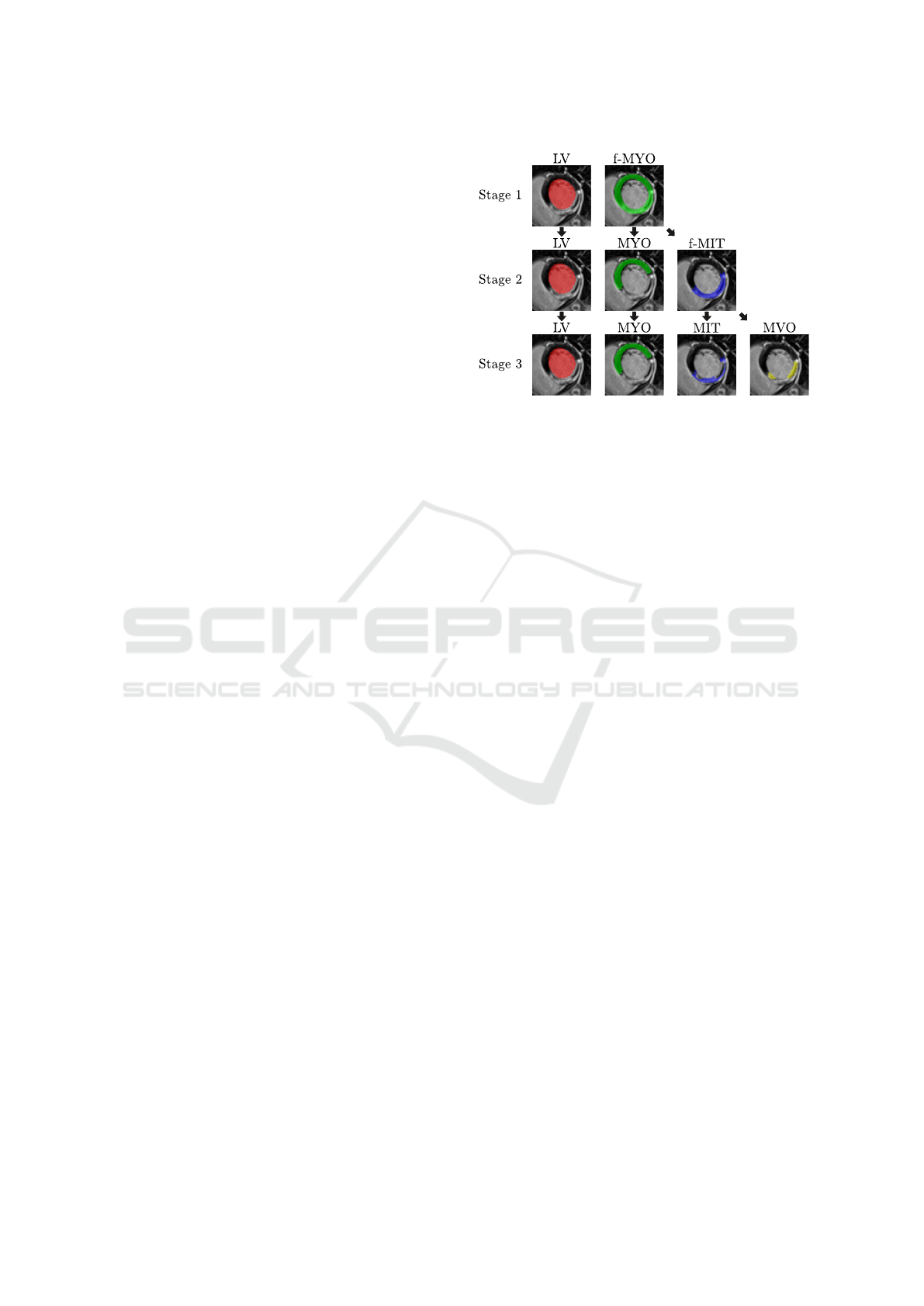
Figure 2: Visualization of the hierarchical label deﬁnitions

per stage as used by CaRe-CNN. While LV remains un-

changed, f-MYO can be separated into MYO and f-MIT of

which the latter can be separated into MIT and MVO.

information. By denoting the Stage 1 model as M

(·)

with trainable parameters θ

, the output prediction

of Stage 1 for image x can be expressed as:

= M

(x;θ

). (1)

Please note that the output prediction

p refers to the

model output without activation function. In Stage 2,

CaRe-CNN learns to predict the LV, the healthy

MYO, the f-MIT and the background by reﬁning the

Stage 1 prediction. To allow consecutive reﬁnement

in Stage 2, we provide

concatenated with the

original image x in the channel dimension as input to

the Stage 2 model. This way,

can be reﬁned based

on the original image information which is crucial for

our cascading CNN as the label deﬁnition of the in-

dividual stages is not the same. The Stage 2 model

(·) with trainable parameters θ

is deﬁned as:

= M

(

⊕ x;θ

), (2)

where ⊕ refers to a concatenation in the channel di-

mension and

refers to the output prediction of

Stage 2, again without any activation function. Lastly,

Stage 3 aims to distinguish all labels, i.e., the LV,

MYO, MIT, MVO as well as the background. To con-

tinue our CNN cascade, we concatenate the prediction

and the image x in the channel dimension to pro-

vide both as input to the Stage 3 model M

(·) of our

cascading CNN. Formally, the output prediction

Stage 3 can be expressed as:

= M

(

⊕ x;θ

), (3)

where θ

refers to the trainable parameters of Stage 3

and ⊕ deﬁnes the concatenation operator.

2.3 Training Objective

In our training pipeline the segmentation loss is com-

puted for each stage individually and backpropagation

CaRe-CNN: Cascading Reﬁnement CNN for Myocardial Infarct Segmentation with Microvascular Obstructions

through all stages is allowed to update model weights

in an end-to-end manner for the whole cascade. As

the label deﬁnition varies from stage to stage, we

adapt the ground truth labels such that they follow the

label deﬁnition of the respective stage as deﬁned in

Fig. 2. For every stage, we compute the generalized

Dice loss between the ground truth y and the label

prediction

y = softmax(

p) of that stage. Formally, the

generalized Dice loss L

(·) is expressed as:

(y,

y) = 1 − 2

∑

k=1

∑

m=1

· y

∑

k=1

∑

m=1

+ y

, (4)

where K represents the number of all labels and M is

the number of voxels. The label weight w

for label k

is computed as the ratio of voxels M

with label k in

the ground truth compared to the number of all voxels,

i.e. w

. The square term

is used to account

for class imbalance.

During training only images that actually contain

the MVO label are forwarded through Stage 3 as im-

ages with missing labels might lead to unstable train-

ing which can greatly impact the performance at that

stage. In order to provide a loss at every stage for ev-

ery iteration while also allowing all training images to

be selected at some point, we always randomly pick

two training images per iteration: One image with and

one without the MVO label. The overall training ob-

jective of CaRe-CNN for all stages and a single image

can then be expressed as:

L(y,

y) = λ

;θ

)

| {z }

update M

+λ

;θ

,θ

)

| {z }

update M

and M

+ δ

MVO

· λ

;θ

,θ

)

| {z }

update M

, M

and M

(5)

where the stage weights λ

, λ

and λ

serve as

weights between the individual loss terms and are set

to 1. The term δ

MVO

is set to 1 if ground truth y con-

tains MVO anywhere and is 0 otherwise. Finally, we

provide the mean loss over the batch to the optimizer.

2.4 Inference

As the subgroup (D8, M1, M12) for every image in

the test set is known as well, we utilize the subgroup

information for test set data to determine the ﬁnal pre-

diction as encouraged by the MYOSAIQ challenge

organizers. Speciﬁcally, we consider the label pre-

diction

of Stage 3 as the ﬁnal label prediction

only for D8 data, while we use the Stage 2 label pre-

diction

as the ﬁnal label prediction

for M1 and

Apex Base

Pred.

w PP

Unc.

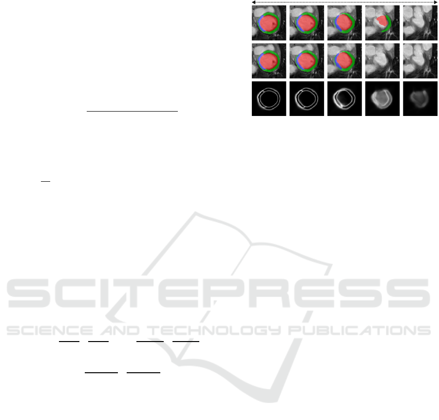
Figure 3: Predictions of CaRe-CNN (row 1) are in some

cases incomplete for the top-most slice towards the base

of the left ventricle (col. 4). The model’s uncertainty is

computed as the entropy of the softmax prediction (row 3),

where bright values indicate a higher uncertainty. The

highest uncertainty occurs in the incompletely labeled slice

(col. 4). This motivates our post-processing (PP) where, in

this case, the incomplete prediction is removed (row 2).

M12 data. The ﬁnal label prediction

is deﬁned as:

(

if x ∈ {M1, M12}

if x ∈ {D8}.

(6)

To further improve the ﬁnal prediction of our method,

we independently trained N = 10 CaRe-CNNs with

random weight initialization and random data aug-

mentation. These N models were used as an ensem-

ble for which the ﬁnal label prediction is obtained by

averaging the ﬁnal label predictions of the individual

models. The average inference time per image for the

whole ensemble with post-processing takes roughly

8 seconds using an NVIDIA GeForce RTX 3090.

2.5 Post-Processing

As can be observed in Fig. 3 (bottom row), after train-

ing on the data our CaRe-CNN remains ’uncertain’

about how far the heart should be segmented towards

the base which may result in a top-most slice that is

incompletely labeled. Even though such incomplete

model predictions in themselves are not incorrect,

we decided to implement a series of post-processing

steps to obtain more consistent predictions that take

anatomical constraints into account.

As a ﬁrst step of our post-processing pipeline, we

employ a disconnected component removal strategy,

where any components that are disconnected from

the largest component in 3D as well as in-plane in

2D are removed. In 3D, a connected component

analysis is performed where all foreground labels are

treated as one label and a 3D 6-connected kernel is

applied. Any independent region that is disconnected

from the largest connected component is removed.

VISAPP 2024 - 19th International Conference on Computer Vision Theory and Applications

Prediction

w Post-P.

Figure 4: CaRe-CNN predictions before (row 1) and after (row 2) post-processing. Images refer to the proposed disconnected

component removal (col. 1), the top-most slice removal (col. 2-4) and the outlier region replacement (col. 5-6). Red arrows

indicate regions of interest.

Due to the large slice thickness of the data, we also

perform a connected component analysis for every

in-plane 2D slice independently, following the same

steps as described for the 3D variant and using a 2D

4-connected kernel in-plane. The 2D strategy mostly

affects the topmost slice that still contains foreground

predictions and removes some smaller in-plane dis-

connected regions from that slice, see Fig. 4 (col. 1).

Next, we propose a top-most slice removal strat-

egy, where we compare the remaining foreground vol-

ume of the topmost slice that contains foreground pre-

dictions to the foreground volume of its neighboring

slice towards the hearts’ apex (i.e. the slice ’below’

the top-most slice). In case that the volume of the

topmost slice is less than half the neighboring slice’s

volume, the topmost slice is removed completely. An

example is shown in Fig. 4 (col. 4).

Lastly, an outlier region replacement strategy is

applied, where very small regions of a single label

are treated as outliers and are replaced if they are iso-

lated from larger regions of the same label. In the

ﬁrst step of this strategy, isolated regions are identi-

ﬁed by performing a connected component analysis

per label using a 3D 6-connected kernel. Any region

with a volume smaller than 0.1 ml is considered to

be an outlier and undergoes a correction step, where

the local neighborhood of each outlier voxel is ob-

served to select a new label for that voxel, see Fig. 4

(col. 5-6). Speciﬁcally, we obtain label votes from

all voxels within a 3D kernel of size 9 × 9 in-plane

and 5 out-of-plane, due to the large slice thickness.

This anisotropic kernel is sufﬁcient as we perform a

weighting based on a 3D Gaussian with sigma value 2

that considers the actual physical distance of any can-

didate. Importantly, votes from voxels marked as out-

liers are not considered. Finally, the maximum of the

weighted votes indicates the most likely label for that

voxel, which is then used as the label for that voxel.

3 EXPERIMENTAL SETUP

3.1 Dataset

In this work, we used the publicly available dataset

from the MYOSAIQ challenge

, which was held in

conjunction with FIMH 2023. The aim of the MYO-

SAIQ challenge is to automatically segment four dif-

ferent cardiac structures from LGE MR images of pa-

tients after myocardial infarction. These structures

encompass the LV, MYO, MIT and MVO if present.

The dataset consists of 467 LGE MR images which

are split into 376 training and 93 test images. All im-

ages belong to one of three subgroups. The ﬁrst sub-

group (D8) encompasses LGE images of 123 patients

with acute myocardial infarction up to eight days

after the infarction and originates from the MIMI-

cohort (Belle et al., 2016). The second subgroup (M1)

consists of LGE images of 204 patients, while the

third subgroup (M12) contains LGE images of 140

patients, which were respectively obtained one and 12

months after coronary intervention and are part of the

HIBISCUS-cohort. For every image in the training

dataset, a corresponding ground truth segmentation is

available. As the whole dataset consists of images

after myocardial infarction, all ground truth segmen-

tations in the dataset contain the LV, MYO and MIT

label. However, the MVO label is exclusive to the D8

subgroup and only present in roughly 66% of the D8

data. The in-plane physical resolution of the dataset

varies from 0.9 to 2.2 mm and averages at 1.57 mm.

Out-of-plane, the physical resolution varies from 5 to

8 mm.

https://www.creatis.insa-lyon.fr/Challenge/myosaiq/,

last accessed on October 8, 2023

CaRe-CNN: Cascading Reﬁnement CNN for Myocardial Infarct Segmentation with Microvascular Obstructions

3.2 Data Augmentation

We augment training data using the training frame-

work from (Payer et al., 2017; Payer et al., 2019)

in 3D using random spatial and intensity transforma-

tions. Spatially, we perform translation (±20 vox-

els), rotation (±0.35 radians), scaling (ﬁrst isotropi-

cally with a factor between [0.8,1.2], then per dimen-

sion with a factor between [0.9,1.1]) and elastic de-

formation (eight grid nodes per dimension, deforma-

tion values are sampled from ±15 voxels). For robust

intensity normalization of the MR images, the 10

and 90

percentile are linearly normalized to −1 and

1, respectively. After normalization, a random inten-

sity shift (±0.2) as well as an intensity scaling with

a factor between [0.6,1.4] is applied to the training

image before modulating intensity values per label by

an additional shift of (±0.2) and scaling with a factor

of [0.9, 1.1]. All augmentation parameters are sam-

pled uniformly from the respective value range. Im-

ages of the test set are not augmented, however, they

are robustly normalized identically to the training data

to ensure similar intensity ranges. To ensure consis-

tency of the physical dimensions across the dataset,

all training and test images are trilinearly resampled

to an isotropic spacing of 1 × 1 ×1 mm and an image

size of 128 × 128 × 128 voxel before being provided

to the CaRe-CNN model.

3.3 Implementation Details

At each stage of CaRe-CNN, a U-Net-like (Ron-

neberger et al., 2015) network architecture is em-

ployed in 3D which follows the same structure, see

Fig. 1. Similar to an encoder-decoder, the architecture

can be separated into a contracting and an expanding

path. Importantly, by using skip-connections, the out-

put of each level of the contracting path is concate-

nated to the input of the same level of the expand-

ing path in the channel dimension. At each of the

ﬁve levels of the contracting and the expanding path,

we use a single block consisting of two convolutions

with an intermediate dropout layer (Srivastava et al.,

2014), after which a pooling or an upsampling layer

is employed, respectively. Two respectively three ad-

ditional convolution layers are employed before and

after the U-Net-like network of each stage. All in-

termediate convolution layers use a 3 × 3 × 3 kernel

and 64 ﬁlters, while the last convolution layer of each

stage uses a 1 × 1 × 1 kernel and as many ﬁlters as

there are labels at the respective stage. He initializa-

tion (He et al., 2015) is used to initialize all weights

and the dropout rate is 0.1. We employ max pooling

layers and tri-linear upsampling layers with a kernel

size of 2 × 2 × 2. Leaky ReLU (Maas et al., 2013)

with a slope of 0.1 is used after intermediate convolu-

tion layers, while a softmax activation is used after the

last layer of each stage to compute the loss. As opti-

mizer, we employ Adam (Kingma and Ba, 2015) with

a learning rate of 0.001, use an Exponential Moving

Average strategy (Laine and Aila, 2016) with a decay

of 0.999 and train for 200, 000 iterations. For each

training iteration, we select one image with and one

without the MVO label which corresponds to a batch

size of 2 for the Stage 1 and Stage 2 models. To ensure

stable training, only images with the MVO label are

processed by the Stage 3 model, which results in an

effective batch size of 1 for that model. During the de-

velopment of our method, we trained our model only

on 2/3 of the training data and used the remaining

1/3 of the data as a validation set. For our submission

to the challenge, we trained CaRe-CNN on all train-

ing data and evaluation was performed on the hidden

test set. Final results were obtained by averaging the

prediction of a CaRe-CNN ensemble of 10 models on

the test set and 5 models on the validation set.

4 RESULTS

The quantitative evaluation is performed by compar-

ing our CaRe-CNN method to the other 17 partici-

pants of the MYOSAIQ challenge on the hidden test

set. For each participant, we obtained ten metric

scores for each label individually from the ofﬁcial

evaluation platform

, which is publicly available. The

used metrics respectively encompass the mean and

standard deviation of the Dice score (DSC) in percent

as well as the Hausdorff distance (HD) and average

symmetric surface distance (ASSD) in mm. Further-

more, the list of metrics includes the mean correlation

coefﬁcient score (CC), mean absolute error (MAE),

limits of agreement (LOA) and the continuous ranked

probability score (CRPS).

In order to summarize the results, we computed

the mean score over the four labels for each metric

and present them in Table 1 for each participant. This

is also true for the standard deviation of DSC, HD and

ASSD, where we also computed the mean score over

the labels. The best score for each metric is given in

bold, while the second and third best metric scores

are shown in underlined blue and italicized orange,

respectively.

Table 2 presents quantitative results per label for

each metric to give some insight into the individual

scores. In the interest of space, we only provide the

https://codalab.lisn.upsaclay.fr/competitions/13631,

last accessed on October 8, 2023

VISAPP 2024 - 19th International Conference on Computer Vision Theory and Applications

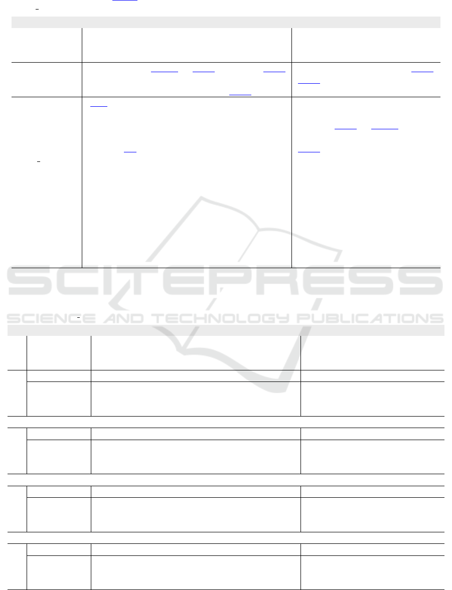
Table 1: Quantitative evaluation showing the mean score over all labels for ten metrics. The proposed CaRe-CNN is com-

pared to the other MYOSAIQ challenge participants. Invalid mean scores due to non-numeric results for at least one label

are indicated by -. The best, second and third best scores are highlighted.

†

Our teamname on the evaluation platform is

’ominous ocelot’.

‡

Abbreviation for ’luiskabongo-inheart’.

Mean over Labels

Team

DSC (%) HD (mm) ASSD (mm)

(↑)

MAE

(↓)

LOA

(↓)

CRPS

(↓)

mean std mean std mean std

(↑) (↓) (↓) (↓) (↓) (↓)

gemr22 74.9 10.3 13.452 7.545 0.711 0.607 0.931 6.044 18.228 0.011

(proposed)

†

78.9 8.5 13.200 9.244 0.574 0.560 0.938 5.500 16.140 0.010

akaroui 75.4 10.0 13.779 8.392 0.697 0.689 0.929 5.827 17.644 0.035

Hairuiwang 75.6 9.8 14.538 9.965 0.711 0.673 0.936 5.810 18.219 0.038

azanella 75.1 10.6 13.483 7.195 0.724 0.685 0.905 5.842 18.337 0.010

KiwiYyy 74.6 12.3 13.771 7.626 0.734 0.702 0.930 5.754 17.247 0.010

hoanguyen93 74.3 11.0 13.905 9.009 0.744 0.758 0.904 5.924 19.297 0.010

nicoco 73.7 9.4 14.839 9.290 0.737 0.630 0.938 6.169 18.044 0.130

hang jung 73.7 9.9 15.063 8.752 0.835 0.766 0.907 6.415 19.802 0.014

Dolphins 73.4 11.9 15.711 10.061 0.754 0.675 0.911 6.578 20.556 0.042

rrosales 73.0 11.0 15.045 8.217 0.856 0.728 0.940 6.788 19.442 0.020

luiskabongo

‡

72.3 10.6 15.584 9.561 0.804 0.718 0.917 7.099 21.622 0.105

calderds 72.0 11.7 17.321 11.853 0.849 0.767 0.909 6.628 20.820 0.039

marwanabb 69.8 12.9 15.667 9.499 1.131 1.183 0.883 7.534 22.477 0.071

agaldran 69.3 19.6 15.947 10.926 - - 0.722 11.712 54.175 -

Erwan 65.5 12.3 20.502 8.416 1.200 1.022 0.853 7.204 22.358 0.012

farheenramzan 55.3 10.6 20.594 9.051 1.641 1.233 0.720 9.349 26.389 0.016

MYOSCANS - - - - - - - - - -

Table 2: Quantitative evaluation showing the individual label scores of the three best MYOSAIQ challenge participants for ten

metrics. ’Overall Best’ refers to the best score obtained by any participant and is used as an upper baseline for each label and

metric. The best score for each metric considering all 18 participants is highlighted in bold.

†

Our teamname on the evaluation

platform is ’ominous ocelot’.

Best 3 Methods per Label

Team

DSC (%) HD (mm) ASSD (mm)

(↑)

MAE

(↓)

LOA

(↓)

CRPS

(↓)

mean std mean std mean std

(↑) (↓) (↓) (↓) (↓) (↓)

Overall Best 93.7 2.8 6.406 2.013 0.392 0.233 0.980 6.881 17.121 0.012

gemr22 93.5 3.1 6.471 2.145 0.408 0.259 0.980 7.308 18.533 0.012

(proposed)

†

93.4 3.4 6.666 2.155 0.419 0.290 0.980 6.881 17.121 0.012

akaroui 93.7 3.0 6.406 2.013 0.392 0.264 0.978 7.313 18.768 0.012

MYO

Overall Best 82.2 4.1 11.753 5.712 0.390 0.211 0.967 7.891 22.251 0.013

gemr22 81.7 4.7 11.794 6.365 0.395 0.246 0.958 9.013 26.664 0.015

(proposed)

†

81.6 5.0 12.839 7.144 0.405 0.253 0.954 9.845 25.686 0.016

akaroui 82.2 4.7 12.214 6.711 0.390 0.259 0.964 8.463 24.263 0.014

MIT

Overall Best 68.4 16.1 16.746 12.482 0.924 1.310 0.855 4.044 17.866 0.007

gemr22 66.0 17.1 18.201 12.482 1.005 1.431 0.799 4.510 20.197 0.008

(proposed)

†

68.4 16.1 16.746 13.414 0.924 1.377 0.833 4.044 18.647 0.007

akaroui 65.8 17.4 19.790 14.751 1.092 1.666 0.789 4.582 20.873 0.008

MVO

Overall Best 72.0 9.5 14.539 5.682 0.547 0.321 0.995 1.231 3.106 0.003

gemr22 58.5 16.4 17.343 9.187 1.037 0.492 0.987 3.343 7.516 0.008

(proposed)

†

72.0 9.5 16.548 14.261 0.547 0.321 0.985 1.231 3.106 0.003

akaroui 59.9 15.0 16.705 10.092 0.913 0.566 0.984 2.950 6.671 0.106

CaRe-CNN: Cascading Reﬁnement CNN for Myocardial Infarct Segmentation with Microvascular Obstructions

Table 3: Ablation of the proposed post-processing (PP) when applied to our CaRe-CNN ensemble predictions. Scores be-

fore (×) and after (✓) post-processing are shown for each label and ten metrics. The last row refers to the mean difference,

where improvements when using post-processing are highlighted in green, while declines are highlighted in red.

Ablation of Proposed CaRe-CNN Ensemble

PP Label

DSC (%) HD (mm) ASSD (mm)

(↑)

MAE

(↓)

LOA

(↓)

CRPS

(↓)

mean std mean std mean std

(↑) (↓) (↓) (↓) (↓) (↓)

LV 93.4 3.3 6.892 2.157 0.422 0.294 0.980 6.837 17.215 0.011

MYO 81.6 4.8 12.088 6.611 0.400 0.238 0.957 9.944 25.271 0.016

MIT 68.5 15.9 16.892 13.46 0.901 1.346 0.837 4.000 18.491 0.007

MVO 71.7 10.0 17.569 13.853 0.576 0.329 0.985 1.210 3.104 0.003

✓

LV 93.4 3.4 6.666 2.155 0.419 0.290 0.980 6.881 17.121 0.012

MYO 81.6 5.0 12.839 7.144 0.405 0.253 0.954 9.845 25.686 0.016

MIT 68.4 16.1 16.746 13.414 0.924 1.377 0.833 4.044 18.647 0.007

MVO 72.0 9.5 16.548 14.261 0.547 0.321 0.985 1.231 3.106 0.003

Mean Diff. +0.1 0 -0.161 +0.223 -0.001 +0.009 -0.002 +0.003 +0.120 +0.000

scores for the three best performing methods in the

challenge as announced at the FIMH 2023 confer-

ence. Nevertheless, to indicate the overall best score

over all teams for each metric and label, we addition-

ally show the best score obtained by any participant

as an upper bound baseline. The best score for each

metric when considering all 18 challenge participants

is given in bold.

Table 3 shows an ablation of the proposed CaRe-

CNN ensemble with and without post-processing.

Again, the scores were obtained from the evaluation

platform of the challenge, where we submitted our

prediction results from the exact same models with

and without post-processing. We show the score for

each label and all metrics evaluated in the challenge.

The last row represents the mean difference between

the scores obtained with and without post-processing.

Underlined green numbers indicate an improvement

and red numbers refer to a decline in performance

when post-processing is applied compared to when it

is not.

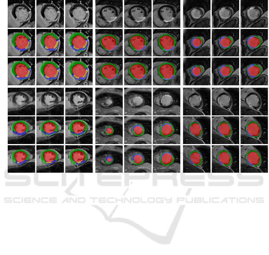
The qualitative evaluation of our CaRe-CNN is

performed by visually inspecting the predictions. As

ground truth segmentations for the test set data are

hidden, we also present qualitative results of CaRe-

CNN trained on 2/3 and validated on 1/3 of the actual

training data for the MYOSAIQ challenge in Fig. 5 to

allow a comparison of our predictions to the ground

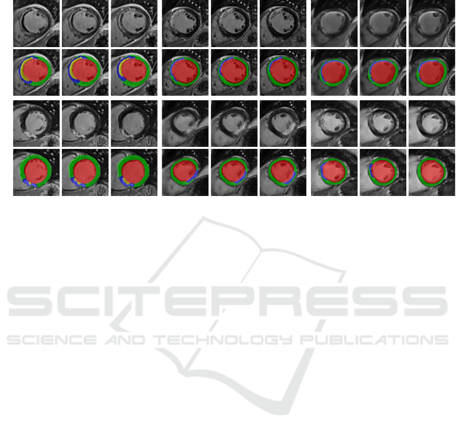
truth. Additionally, we provide qualitative results of

our ﬁnal method submitted to the challenge on the

test set in Fig. 6, however, without publicly available

ground truth segmentations, the predictions are only

compared to the respective input images. Both ﬁgures

show three consecutive slices of two MR scans of pa-

tients after acute MI per subgroup (D8, M1, M12).

5 DISCUSSION

Quantitative Evaluation. The mean score over the

four labels presented in Table 1 shows, that on average

our method achieved the best score for eight out of

ten metrics. Other participants only outperformed our

method on the mean standard deviation of the HD as

well as the CC, where CaRe-CNN obtained a tied sec-

ond best score. Most notably, our method shows great

improvements compared to the other methods on the

DSC and ASSD scores. Speciﬁcally, with a mean

DSC of 78.9%, CaRe-CNN achieved an improvement

of 3.3% compared to the second best method with

75.6%. The same 3.3% window applied to the range

[75.6%,72.3%] encompasses the second up to the 12

best mean DSC score. Similarly, with a result of

0.574 mm on the ASSD score our method achieved

an improvement of 0.123 mm over the second best

ASSD score with 0.697 mm. The second up to the

best score lie within the same 0.123 mm window

of [0.697 mm,0.820 mm].

More details are provided in Table 2, where the

per label scores and the overall best score of any

method are shown. For the LV results, it can be ob-

served that our method obtained the best scores for

MAE and LOA, and obtained tied best scores with

other methods for the CC and CRPS. Moreover, the

shown DSC, HD and ASSD scores are all very close

to one another with our method achieving 93.4%

(best: 93.7%) DSC, 6.67 mm (best: 6.41 mm) HD

and 0.42 mm (best: 0.39 mm) ASSD. On MYO, our

method did not obtain the best score on any metric and

underperformed compared to the overall best score

most notably with 12.839 mm (best: 11.753 mm)

HD, 9.845 (best: 7.891) MAE and 25.686 (best:

22.251) LOA. Nevertheless, on other metrics like

VISAPP 2024 - 19th International Conference on Computer Vision Theory and Applications

Image

GTPred.

Image

GTPred.

D8 M1 M12

Figure 5: Qualitative results of CaRe-CNN on the validation set. Columns refer to three consecutive slices of LGE MR scans

of patients after MI for the three subgroups: D8 (col. 1-3), M1 (col. 4-6) and M12 (7-9). Rows refer to scans of two separate

patients and show the image (rows 1, 4), ground truth (rows 2, 5) and prediction of CaRe-CNN (rows 3, 6).

DSC and ASSD our method remains competitive to

the other methods achieving 81.6% (best: 82.2%)

DSC and 0.405 mm (best: 0.390 mm) ASSD.

Compared to the other challenge participants,

our CaRe-CNN excelled when segmenting the difﬁ-

cult but clinically most relevant MIT and MVO la-

bels, where our method obtained the best score for

six and seven out of the ten metrics, respectively.

Among the three challenge winners, our method

achieved good improvements on the MIT label with

68.4% (+2.4%) DSC, 16.746 mm (−1.455 mm) HD,

0.924 mm (−0.081 mm) ASSD and 4.044 (−0.466)

MAE. Interestingly, our method underperformed on

the HD of the MVO label achieving a mean of

16.548 mm (best: 14.539 mm) and a standard devi-

ation of 14.261 mm (best: 5.682 mm). On other met-

rics, however, CaRe-CNN achieved great improve-

ments for the MVO label compared to the other two

challenge winners, namely 72.0% (+12.1%) DSC,

0.547 mm (−0.366 mm) ASSD, 1.231 (−1.719)

MAE and 3.106 (−3.565) LOA.

Post-Processing. When observing the training data

more closely, we noticed that the ground truth an-

notations of the heart labels towards the base of the

heart are not always complete. Most notably, how far

slices are labeled towards the base varies from image

to image, which is likely an artifact from the anno-

tation protocol. While such incomplete annotations

are not incorrect, they introduce a bias to the dataset

which is reﬂected by a machine learning model and

leads to some expected inconsistencies in the model

predictions. We mitigate these inconsistencies using

a series of post-processing steps to obtain more con-

sistent predictions and show that quantitative scores

for all metrics are almost unchanged in Table 3. The

most affected metric is the HD resulting in a mean

of 13.200 mm (mean difference: −0.161 mm) and

a standard deviation of 9.243 mm (mean difference:

+0.223 mm) after post-processing. This conﬁrms our

expectation, that the top-most slice removal strategy

paired with the large slice thickness of 5.6 mm on av-

erage leads to the HD being the most affected met-

ric as it is deﬁned as the maximum distance of any

voxel-pair of the same label between ground truth and

prediction. Nevertheless, the relative change over all

metrics averages to 0.6% when using post-processing,

which conﬁrms that it can be safely applied in order to

CaRe-CNN: Cascading Reﬁnement CNN for Myocardial Infarct Segmentation with Microvascular Obstructions

Image

Pred.

Image

Pred.

D8 M1 M12

Figure 6: Qualitative results of CaRe-CNN on the test set. Columns refer to three consecutive slices of LGE MR scans of

patients after MI for each subgroup: D8 (col. 1-3), M1 (col. 4-6) and M12 (7-9). Rows refer to scans of two separate patients

and show the image (rows 1, 3) and prediction of CaRe-CNN (rows 2, 4). Ground truth is not available for the test set.

improve the qualitative consistency of the predictions.

Qualitative Evaluation. The qualitative results on

the validation set in Fig. 5 conﬁrm that most label

predictions are very close to the ground truth. On

closer inspection, however, some differences can be

spotted. For example, one of the two MVO regions is

predicted in one additional consecutive slice in con-

trast to the ground truth (D8, top), while the MIT la-

bel is overpredicted close to the apex (M1, bottom).

Also, an MVO label prediction for a patient without

MVO is visible (D8, bottom). Nevertheless, many re-

gions are predicted correctly, most notably even for

data where the wall is in parts only two to three vox-

els thick (M12, bottom). On the test set in Fig. 5,

qualitative results can only be compared to the LGE

MR image. Overall, the label predictions appear to be

realistic which is supported by our quantitative evalu-

ation, however, further conﬁrmation needs to be per-

formed by an expert.

Challenges and Limitations. One major challenge

of correctly segmenting the structures of interest

arises from the limited resolution of the LGE MR

data in combination with the shape and small phys-

ical size of the structures, most notably the MIT and

MVO label. While the LV is comparatively easy to

segment due to its size and blob-like shape in 3D, the

f-MYO label that surrounds the LV averages to a mid-

diastolic thickness of 6.47 ± 1.07 mm in women and

7.90 ± 1.24 mm in men (Walpot et al., 2019) with-

out considering infarction. In a small cohort, (Khalid

et al., 2019) showed that during ejection, healthy wall

segments are roughly three times as thick (8.73 mm)

compared with infarcted wall segments (2.86 mm).

Furthermore, infarction might only affect some part

of the myocardial tissue in transmural direction such

that two or even all three of the f-MYO sublabels

(MYO, MIT and MVO) might be present across the

already thin wall. The in-plane resolution of the LGE

MR data with 1.57 mm on average paired with the

small physical size of some of the structures of inter-

est leads to a potential transmural thickness of only a

few voxels for these labels. Moreover, segmentation

models are inherently uncertain near the label bor-

ders and thus, prone to single voxel errors, which can

strongly affect the scores for small structures like the

MIT and MVO labels. The combination of these ef-

fects explains the disparity of the LV to the MIT and

MVO label scores for which CaRe-CNN achieved the

best score in six (MIT) and seven (MVO) out of ten

metrics among 18 challenge participants.

A remaining challenge arises from the MVO la-

bel predictions for some patients of the D8 subgroup,

where the label was not predicted when it should be

present or vice versa. Since the presence of MVO

is linked to an increased risk of adverse cardiovascu-

lar events (Hamirani et al., 2014; Rios-Navarro et al.,

2019), incorrect predictions of MVO might impact

clinical decision making if trusted blindly. While

manual veriﬁcation by an expert is necessary, our

state-of-the-art predictions can alleviate the manual

workload to obtain correct segmentations of patient-

speciﬁc anatomy.

VISAPP 2024 - 19th International Conference on Computer Vision Theory and Applications

6 CONCLUSION

In this work we presented CaRe-CNN, a 3-stage

cascading reﬁnement CNN, which segments cardiac

LGE MR images after MI. The cascading architec-

ture is designed to exploit the hierarchical label def-

inition of the data and is trained end-to-end fully

in 3D. Furthermore, we employed a series of post-

processing steps that improve the consistency of the

predictions by taking anatomical constraints into ac-

count. The proposed CaRe-CNN was submitted to

the MYOSAIQ challenge, where it ranked second out

of 18 participating teams and achieved state-of-the-art

segmentation results, most notably when segmenting

the difﬁcult MIT and MVO labels. Due to great im-

provements over related work on the difﬁcult but clin-

ically very relevant MVO label, our method obtained

the best score in eight out of ten metrics when com-

puting the mean over all labels. Precise segmenta-

tions of healthy and infarcted myocardial tissue after

MI allow patient-speciﬁc therapy planning and are an

important step towards personalized medicine. In our

future work, we plan to investigate uncertainty quan-

tiﬁcation strategies to further improve CaRe-CNN for

future rounds of the MYOSAIQ challenge.

ACKNOWLEDGEMENTS

This research was funded by the InstaTwin grant

FO999891133 from the Austrian Research Promotion

Agency (FFG).

REFERENCES

Akkus, Z., Galimzianova, A., Hoogi, A., Rubin, D. L., and

Erickson, B. J. (2017). Deep Learning for Brain MRI

Segmentation: State of the Art and Future Directions.

Journal of Digital Imaging, 30:449–459.

Belle, L., Motreff, P., Mangin, L., Rang

e, G., Marcaggi,

X., Marie, A., Ferrier, N., Dubreuil, O., Zemour, G.,

Souteyrand, G., et al. (2016). Comparison of Im-

mediate with Delayed Stenting Using the Minimal-

ist Immediate Mechanical Intervention Approach in

Acute ST-Segment–Elevation Myocardial Infarction:

The MIMI Study. Circulation: Cardiovascular Inter-

ventions, 9(3):e003388.

Campos, F. O., Neic, A., Mendonca Costa, C., Whitaker,

J., O’Neill, M., Razavi, R., Rinaldi, C. A., Scherr,

D., Niederer, S. A., Plank, G., et al. (2022). An Au-

tomated Near-Real Time Computational Method for

Induction and Treatment of Scar-related Ventricular

Tachycardias. Medical Image Analysis, 80:102483.

Chen, C., Qin, C., Qiu, H., Tarroni, G., Duan, J., Bai, W.,

and Rueckert, D. (2020). Deep Learning for Cardiac

Image Segmentation: A Review. Frontiers in Cardio-

vascular Medicine, 7:25.

Chen, Z., Lalande, A., Salomon, M., Decourselle, T., Pom-

mier, T., Qayyum, A., Shi, J., Perrot, G., and Cou-

turier, R. (2022). Automatic Deep Learning-based

Myocardial Infarction Segmentation from Delayed

Enhancement MRI. Computerized Medical Imaging

and Graphics, 95:102014.

Esteva, A., Kuprel, B., Novoa, R. A., Ko, J., Swetter, S. M.,

Blau, H. M., and Thrun, S. (2017). Dermatologist-

level Classiﬁcation of Skin Cancer with Deep Neural

Networks. Nature, 542(7639):115–118.

Fahmy, A. S., Rausch, J., Neisius, U., Chan, R. H., Maron,

M. S., Appelbaum, E., Menze, B., and Nezafat, R.

(2018). Automated Cardiac MR Scar Quantiﬁcation

in Hypertrophic Cardiomyopathy Using Deep Con-

volutional Neural Networks. JACC: Cardiovascular

Imaging, 11(12):1917–1918.

Feng, S., Liu, Q., Patel, A., Bazai, S. U., Jin, C.-K., Kim,

J. S., Sarrafzadeh, M., Azzollini, D., Yeoh, J., Kim,

E., et al. (2022). Automated Pneumothorax Triaging

in Chest X-rays in the New Zealand Population Using

Deep-learning Algorithms. Journal of Medical Imag-

ing and Radiation Oncology, 66(8):1035–1043.

Gillette, K., Gsell, M. A., Prassl, A. J., Karabelas, E., Re-

iter, U., Reiter, G., Grandits, T., Payer, C.,

Stern, D.,

Urschler, M., et al. (2021). A Framework for the Gen-

eration of Digital Twins of Cardiac Electrophysiology

from Clinical 12-leads ECGs. Medical Image Analy-

sis, 71:102080.

Graves, A., Mohamed, A.-r., and Hinton, G. (2013). Speech

Recognition with Deep Recurrent Neural Networks.

In Proceedings of the IEEE International Conference

on Acoustics, Speech and Signal Processing, pages

6645–6649.

Hamirani, Y. S., Wong, A., Kramer, C. M., and Salerno,

M. (2014). Effect of Microvascular Obstruction and

Intramyocardial Hemorrhage by CMR on LV Remod-

eling and Outcomes after Myocardial Infarction: A

Systematic Review and Meta-Analysis. JACC: Car-

diovascular Imaging, 7(9):940–952.

He, K., Zhang, X., Ren, S., and Sun, J. (2015). Delving

Deep into Rectiﬁers: Surpassing Human-Level Per-

formance on ImageNet Classiﬁcation. In Proceedings

of the IEEE International Conference on Computer

Vision, pages 1026–1034.

Hellermann, J. P., Jacobsen, S. J., Gersh, B. J., Rodeheffer,

R. J., Reeder, G. S., and Roger, V. L. (2002). Heart

Failure after Myocardial Infarction: A Review. The

American Journal of Medicine, 113(4):324–330.

Khalid, A., Lim, E., Chan, B. T., Abdul Aziz, Y. F., Chee,

K. H., Yap, H. J., and Liew, Y. M. (2019). Assess-

ing Regional Left Ventricular Thickening Dysfunction

and Dyssynchrony via Personalized Modeling and 3D

Wall Thickness Measurements for Acute Myocardial

Infarction. Journal of Magnetic Resonance Imaging,

49(4):1006–1019.

Kim, R. J., Fieno, D. S., Parrish, T. B., Harris, K., Chen,

E.-L., Simonetti, O., Bundy, J., Finn, J. P., Klocke,

F. J., and Judd, R. M. (1999). Relationship of MRI

Delayed Contrast Enhancement to Irreversible Injury,

CaRe-CNN: Cascading Reﬁnement CNN for Myocardial Infarct Segmentation with Microvascular Obstructions

Infarct Age, and Contractile Function. Circulation,

100(19):1992–2002.

Kim, R. J. and Manning, W. J. (2004). Viability Assess-

ment by Delayed Enhancement Cardiovascular Mag-

netic Resonance: Will Low-dose Dobutamine Dull the

Shine? Circulation, 109(21):2476–2479.

Kingma, D. P. and Ba, J. L. (2015). Adam: A Method for

Stochastic Optimization. In Proceedings of the Inter-

national Conference on Learning Representations.

Laine, S. and Aila, T. (2016). Temporal Ensembling for

Semi-Supervised Learning. In Proceedings of the In-

ternational Conference on Learning Representations.

Lalande, A., Chen, Z., Pommier, T., Decourselle, T.,

Qayyum, A., Salomon, M., Ginhac, D., Skan-

darani, Y., Boucher, A., Brahim, K., et al. (2022).

Deep Learning Methods for Automatic Evaluation

of Delayed Enhancement-MRI. The Results of the

EMIDEC Challenge. Medical Image Analysis,

79:102428.

Maas, A. L., Hannun, A. Y., and Ng, A. Y. (2013). Recti-

ﬁer Nonlinearities Improve Neural Network Acoustic

Models. In Proceedings of the International Confer-

ence on Machine Learning, volume 30, page 3. At-

lanta, GA.

Moccia, S., Banali, R., Martini, C., Muscogiuri, G., Pon-

tone, G., Pepi, M., and Caiani, E. G. (2019). Develop-

ment and Testing of a Deep Learning-based Strategy

for Scar Segmentation on CMR-LGE Images. Mag-

netic Resonance Materials in Physics, Biology and

Medicine, 32:187–195.

Payer, C.,

Stern, D., Bischof, H., and Urschler, M. (2017).

Multi-label Whole Heart Segmentation using CNNs

and Anatomical Label Conﬁgurations. In Interna-

tional Workshop on Statistical Atlases and Computa-

tional Models of the Heart, pages 190–198. Springer.

Payer, C.,

Stern, D., Bischof, H., and Urschler, M. (2019).

Integrating Spatial Conﬁguration into Heatmap Re-

gression based CNNs for Landmark Localization.

Medical Image Analysis, 54:207–219.

Payer, C.,

Stern, D., Bischof, H., and Urschler, M. (2020).

Coarse to Fine Vertebrae Localization and Segmenta-

tion with SpatialConﬁguration-Net and U-Net. In 15th

International Joint Conference on Computer Vision,

Imaging and Computer Graphics Theory and Applica-

tions (VISIGRAPP 2020) - Volume 5: VISAPP, pages

124–133.

Perin, E. C., Silva, G. V., Sarmento-Leite, R., Sousa, A. L.,

Howell, M., Muthupillai, R., Lambert, B., Vaughn,

W. K., and Flamm, S. D. (2002). Assessing My-

ocardial Viability and Infarct Transmurality with Left

Ventricular Electromechanical Mapping in Patients

with Stable Coronary Artery Disease: Validation by

Delayed-Enhancement Magnetic Resonance Imaging.

Circulation, 106(8):957–961.

Rios-Navarro, C., Marcos-Garces, V., Bayes-Genis, A.,

Husser, O., Nunez, J., and Bodi, V. (2019). Mi-

crovascular Obstruction in ST-segment Elevation My-

ocardial Infarction: Looking Back to Move For-

ward. Focus on CMR. Journal of Clinical Medicine,

8(11):1805.

Ronneberger, O., Fischer, P., and Brox, T. (2015). U-Net:

Convolutional Networks for Biomedical Image Seg-

mentation. In Proceedings of the International Con-

ference on Medical Image Computing and Computer-

Assisted Intervention, pages 234–241.

Rosenthal, M. E., Oseran, D. S., Gang, E., and Peter,

T. (1985). Sudden Cardiac Death following Acute

Myocardial Infarction. American Heart Journal,

109(4):865–876.

Schinkel, A. F., Poldermans, D., Elhendy, A., and Bax,

J. J. (2007). Assessment of Myocardial Viability

in Patients with Heart Failure. Journal of Nuclear

Medicine, 48(7):1135–1146.

Selvanayagam, J. B., Kardos, A., Francis, J. M., Wiesmann,

F., Petersen, S. E., Taggart, D. P., and Neubauer,

S. (2004). Value of Delayed-enhancement Cardio-

vascular Magnetic Resonance Imaging in Predicting

Myocardial Viability after Surgical Revascularization.

Circulation, 110(12):1535–1541.

Srivastava, N., Hinton, G., Krizhevsky, A., Sutskever, I.,

and Salakhutdinov, R. (2014). Dropout: A Sim-

ple Way to Prevent Neural Networks from Overﬁt-

ting. The Journal of Machine Learning Research,

15(1):1929–1958.

Van der Wall, E., Vliegen, H., De Roos, A., and Bruschke,

A. (1996). Magnetic Resonance Techniques for As-

sessment of Myocardial Viability. Journal of Cardio-

vascular Pharmacology, 28:37–44.

Walpot, J., Juneau, D., Massalha, S., Dwivedi, G., Rybicki,

F. J., Chow, B. J., and In

acio, J. R. (2019). Left Ven-

tricular Mid-diastolic Wall Thickness: Normal Values

for Coronary CT Angiography. Radiology: Cardio-

thoracic Imaging, 1(5):e190034.

Wroblewski, L. C., Aisen, A. M., Swanson, S. D., and

Buda, A. J. (1990). Evaluation of Myocardial Vi-

ability following Ischemic and Reperfusion Injury

using Phosphorus 31 Nuclear Magnetic Resonance

Spectroscopy in Vivo. American Heart Journal,

120(1):31–39.

Xu, C., Wang, Y., Zhang, D., Han, L., Zhang, Y., Chen,

J., and Li, S. (2022). BMAnet: Boundary Mining

with Adversarial Learning for Semi-supervised 2D

Myocardial Infarction Segmentation. IEEE Journal

of Biomedical and Health Informatics, 27(1):87–96.

Xu, C., Xu, L., Gao, Z., Zhao, S., Zhang, H., Zhang, Y., Du,

X., Zhao, S., Ghista, D., Liu, H., et al. (2018). Direct

Delineation of Myocardial Infarction without Contrast

Agents using a Joint Motion Feature Learning Archi-

tecture. Medical Image Analysis, 50:82–94.

Zabihollahy, F., White, J. A., and Ukwatta, E. (2018). My-

ocardial Scar Segmentation from Magnetic Resonance

Images using Convolutional Neural Network. In Med-

ical Imaging 2018: Computer-Aided Diagnosis, vol-

ume 10575, pages 663–670. SPIE.

Zhang, Y. (2021). Cascaded Convolutional Neural Network

for Automatic Myocardial Infarction Segmentation

from Delayed-enhancement Cardiac MRI. In Interna-

tional Workshop on Statistical Atlases and Computa-

tional Models of the Heart, pages 328–333. Springer.

VISAPP 2024 - 19th International Conference on Computer Vision Theory and Applications