Compositional Techniques for Asynchronous Boolean Networks

Maram Alshahrani

1,2 a

and Jason Steggles

1 b

School of Computing, Newcastle University, Newcastle upon Tyne, U.K.

Faculty of Computer Science, King Khalid University, Abha, Saudi Arabia

Keywords:

Asynchronous Boolean Networks, Model Composition, Behaviour Preservation, Attractor Identiﬁcation.

Abstract:

Asynchronous Boolean networks are an important qualitative modelling approach for analysing and engineer-

ing biological systems. However, their practical application is limited by the state space explosion problem

and lack of engineering tools. To help address these limitations we develop new compositional techniques

for constructing and analysing asynchronous Boolean networks based on the idea of merging entities using

Boolean operators. We propose a novel asynchronous interference state graph to model the interference that

occurs in a composition and develop a range of important new asynchronous compositional techniques for

analysing behavioural preservation and identifying point attractors.

1 INTRODUCTION

Boolean networks (Kauffman, 1969) are a widely

studied qualitative modelling approach (Barbuti et al.,

2020) that has been successfully applied to a range of

biological systems (for example, see (Pandey et al.,

2010; Dahlhaus et al., 2016)). A Boolean network

abstractly represents the state of regulatory entities as

Boolean values and provides update rules to capture

how these entities interact. They can provide key in-

sights into the behaviour of a regulatory system by

considering the attractors (state cycles) they exhibit

(for example, see (Huang and Ingber, 2000; Saadat-

pour et al., 2011)). The global state of a Boolean net-

work can be updated either synchronously (all entities

update their state simultaneously) or asynchronously

(entities update their state independently and non-

deterministically) (Schwab et al., 2020). While the

synchronous update scheme provides more tractable

analysis, the asynchronous update scheme is gener-

ally seen to allow more realistic dynamic behaviour

(Barbuti et al., 2020).

The practical application of Boolean networks is

limited by the state space explosion problem (Groote

et al., 2015) (exponential growth of state space) and

by the lack of engineering techniques. In this paper

we make an important contribution to supporting the

practical application of asynchronous Boolean net-

https://orcid.org/0009-0005-0793-0504

https://orcid.org/0000-0001-9174-5531

works by developing formal techniques for their com-

positional construction and analysis. We take as our

starting point an approach for composing syn-

chronous Boolean networks based on merging en-

tities between submodels using Boolean operators

(Alkhudhayr and Steggles, 2019; Abdulrahman and

Steggles, 2023). Adapting this approach to the asyn-

chronous setting involves dealing with the fundamen-

tal semantic differences between synchronous and

asynchronous updating schemes and has led to a

range of important new insights and results.

We begin by developing a new form of interfer-

ence state graph (Alkhudhayr and Steggles, 2019)

for the asynchronous setting which captures the inter-

ference that can occur to a Boolean network’s asyn-

chronous behaviour in a composition. We prove this

interference state graph bounds the asynchronous be-

haviour possible for a submodel in a composition and

then develop key results about the preservation of a

submodel’s behaviour in a composition.

We further strengthen our asynchronous compo-

sitional framework by developing new compositional

techniques for identifying point attractors (Hopfen-

sitz et al., 2013) (global states with no outgoing transi-

tions) in an asynchronous composition. We formulate

an approach based on identifying and combining po-

tential self-loops in the submodels, taking account of

the impact that interference can have. The results here

are promising and importantly provide a foundation

for developing general techniques and tools for com-

positionally identifying cyclic and complex attractors.

Alshahrani, M. and Steggles, J.

Compositional Techniques for Asynchronous Boolean Networks.

DOI: 10.5220/0012324300003657

Paper published under CC license (CC BY-NC-ND 4.0)

In Proceedings of the 17th International Joint Conference on Biomedical Engineering Systems and Technologies (BIOSTEC 2024) - Volume 1, pages 429-437

ISBN: 978-989-758-688-0; ISSN: 2184-4305

429

2 BACKGROUND

2.1 Boolean Networks

A Boolean network (Kauffman, 1969) is a qualitative

modelling approach which consists of a set of regula-

tory entities that have a Boolean state. Each entity has

a next-state update function that deﬁnes its behaviour

based on the state of its related entities.

Deﬁnition 1. A Boolean network BN is a tuple

BN = (G,N,F) where:

i) G = {g

,...,g

} is a non-empty, ﬁnite set of en-

tities;

ii) N = (N(g

),N(g

),...,N(g

)) is a tuple of neigh-

bourhoods, such that N(g

) ⊆ G is the neighbourhood

of g

;

iii) F = (F(g

),F(g

),..., F(g

)) is a tuple of next-

state functions, where F(g

) : B

|N(g

→ B deﬁnes the

next state of g

We deﬁne a global state of a Boolean network BN

to be a function S : G → B, where S(g) represents the

state of entity g ∈ G, and we let S

= [G → B] repre-

sent the set of all global states. If a Boolean network

has n ∈ N entities then S

will contain 2

states

and this indicates that Boolean networks are impacted

by the state space explosion problem (Groote et al.,

2015). Given a global state S ∈ S

and a subset of

entities X ⊆ G we deﬁne the projection of S over X to

be the function S[X] : X → B, where S[X](g) = S[g],

for any g ∈ X. For any S ∈ S

, g ∈ G and b ∈ B we

let S[g → b] denote the state update which results in

a new global state where S[g → b](h) = S(h), for all

h ∈ G, h ̸= g, and S[g → b](g) = b.

A range of update semantics exist for Boolean

networks and two key approaches are: synchronous,

where all entities update their state simultaneously;

and asynchronous, where each entity updates its state

independently and non-deterministically (Schwab

et al., 2020). The asynchronous semantics can be seen

to capture more realistic dynamic behaviour (Barbuti

et al., 2020) and we focus on this.

Deﬁnition 2. Given global states S,S

′

∈ S

, we

say S

−−→ S

′

is an asynchronous update step iff ex-

ists g ∈ G such that S

′

(g) = ¬S(g) = F(g)(S[N(g)])

and S(h) = S

′

(h), for all h ∈ G, h ̸= g. We let

(S) = {S

′

| S

′

∈ S

, and S

−−→ S

′

}. The com-

plete asynchronous behaviour of a Boolean network is

concisely captured by the (asynchronous) state graph

SG(BN ) = (S

−−→).

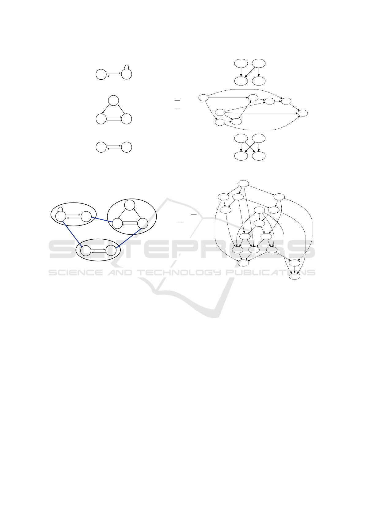
For illustrative examples, consider the Boolean

networks presented in Figure 1.

A path in the asynchronous state graph SG(BN )

represents one possible sequence of behaviour and

can be ﬁnite or inﬁnite (this contrasts with the syn-

chronous setting where all paths are inﬁnite (Kauff-

man et al., 1993)). We let Path(SG(BN )) denote

the set of all paths over SG(BN ). Given α ∈

Path(SG(BN )) we let SD(α) represent the step do-

main of α, where SD(α) = {0, ..., k − 1} if α :

{0,.. .,k} → S

is a ﬁnite path and SD(α) = N if

α : N → S

is an inﬁnite path.

A global state with no update steps is known as

a point attractor and other complex, cyclic attractors

can be considered (Schwab et al., 2020; Hopfensitz

et al., 2013). Attractors provide important insights

into a model’s behaviour and can be associated with

biological phenomena (Huang and Ingber, 2000).

2.2 A Compositional Framework

A range of approaches for composing and decom-

posing Boolean networks for analysis have been pro-

posed (for example, see (Alkhudhayr and Steggles,

2019; Zhao et al., 2013; Mizera et al., 2017)). We fo-

cus on recent work which presents a novel approach

to composing synchronous Boolean networks based

on merging entities between Boolean networks using

Boolean operators (Alkhudhayr and Steggles, 2019;

Abdulrahman and Steggles, 2023). They focused

solely on the synchronous update semantics and de-

veloped a range of interesting techniques and tools for

analysing composed synchronous Boolean networks.

We brieﬂy introduce key concepts from this com-

positional framework needed in the sequel. We only

consider using conjunction for merging entities in the

sequel but note that all the results presented also hold

for disjunction. We begin by recalling the deﬁnition

of a composition (Abdulrahman and Steggles, 2023).

Deﬁnition 3. A composition Σ = (M,E), where M =

{BN

,BN

,...,BN

} is the set of Boolean networks

(submodels) that are used in the composition Σ, for

some n ∈ N, n > 1, and E deﬁnes merged entities

E ⊆ {{g

} | BN

,BN

∈ M, BN

̸= BN

and

∈ G

, g

∈ G

}

As an illustrative example, consider the com-

position Σ

= (M

) presented in Figure 2,

where M

= {BN

Ex1

,BN

Ex2

,BN

Ex3

}, and E

{{g

},{g

}}.

In order to reason about a composition we intro-

duce the following important notations and deﬁni-

tions. We let gc(Σ,BN

) represent the set of enti-

ties from BN

that are composed in Σ and deﬁne it

as gc(Σ,BN

) = {g | g ∈ G

and {g,g

′

} ∈ E}. We let

gc(Σ) = gc(Σ,BN

) ∪ ... ∪ gc(Σ, BN

) represent the

set of all entities that are composed in Σ.

BIOINFORMATICS 2024 - 15th International Conference on Bioinformatics Models, Methods and Algorithms

430

Ex1

] = g

∨ g

Ex2

] = g

∧ g

] = g

000 010

011

001

101

100110

111

Ex3

] = g

11 00

Figure 1: The interaction diagram, next-state functions and the state graph for three example Boolean networks BN

Ex1

Ex2

and BN

Ex3

Ex1

Ex2

Ex3

] = g

∧ (g

∧ g

)

] = g

∧ g

] = (g

∨ g

) ∧ g

] = g

0001

0000

0010

0110

0111

0011

1011

1001 1010

0100

0101

1000

1100

11101101

1111

Figure 2: An example composition Σ

in which three Boolean networks BN

Ex1

, BN

Ex2

and BN

Ex3

are composed, where

the resulting compositional entities (represented by thick blue edges) are g

= {g

}, g

= {g

} and g

= {g

}. The

asynchronous state graph is also depicted for the resulting Boolean network BN (Σ

For any g ∈ gc(Σ) we let ∆(g) denote the set of all

entities that are composed with g (including g itself).

We let λ(g) denote the index of the Boolean net-

work that g belongs to. For any i ∈ {1, ... , n} and any

g ∈ G

we deﬁne λ(g) = i.

We let Σ(g) be the renaming used to move

between a submodel and the composition deﬁned

for any entity g ∈ (G

∪ ... ∪ G

) by Σ(g) = g, if

g /∈ gc(Σ); or Σ(g) = ∆(g), otherwise.

A composition Σ results in a Boolean network

BN (Σ) (Abdulrahman and Steggles, 2023).

Deﬁnition 4. Let Σ = (M,E) be a composition.

Then we deﬁne the Boolean network BN (Σ) =

(G(Σ),N(Σ),F(Σ)) that results from Σ as follows.

1. Entities: G(Σ) = Σ(G

∪ ... ∪ G

2. Neighbourhood: for any entity h ∈ G(Σ), we deﬁne

the neighbourhood N(Σ)(h) by

N(Σ)(h) =

g∈h

Σ(N

λ(g)

(g)),

if h = ∆(g

′

), for some g

′

∈ gc(Σ); or N(Σ)(h) =

Σ(N

λ(h)

(h)), otherwise.

3. Functions: For any entity g ∈ G(Σ), we deﬁne the

next–state function F(Σ)(g) on any S ∈ S

BN (Σ)

F(Σ)(g)(S[N(Σ)(g)]) =

h∈∆(g

′

)

λ(h)

(h)(S[Σ(N

λ(h)

(h))]),

if g = ∆(g

′

), for some g

′

∈ gc(Σ); or

F(Σ)(g)(S[N(Σ)(g)]) = F

λ(g)

(g)(S[Σ(N

λ(g)

(g))]),

otherwise.

For an example, see Figure 2 where the composed

model BN (Σ

) resulting from Σ

is shown. In a

slight abuse of notation we use the set of entities com-

posed as the name of the resulting composed entity.

In the sequel we use the above deﬁnitions for our

asynchronous compositional theory but place an im-

portant restriction on a composition’s graph structure

Compositional Techniques for Asynchronous Boolean Networks

431

to ensure that no two entities in an asynchronous sub-

model are composed together (since this would result

in synchronous behaviour).

2.3 Related Work

The compositional framework for asynchronous

Boolean networks we present is based on the novel

idea of composing synchronous Boolean networks by

merging entities using a Boolean operator (Alkhud-

hayr and Steggles, 2019; Abdulrahman and Steggles,

2023). However, the work presented here takes a sig-

niﬁcantly different approach as required by our focus

on asynchronous models.

There are some interesting studies on behaviour

preservation and subnetwork embeddings in the liter-

ature (for example, see (Thomas and d’Ari, 1990)) but

the approach we take is new.

A range of research into the composition and de-

composition of Boolean networks can be found in the

literature, e.g. (Tournier and Chaves, 2013; Dubrova

and Teslenko, 2005; Cheng et al., 2012; Zhao et al.,

2013). The approaches taken by these papers appear

to be signiﬁcantly different to our work and focus on

applying decomposition/composition to aid identify-

ing the attractors of a Boolean network. They ap-

pear not to consider developing a general composi-

tional framework for constructing and analysing asyn-

chronous Boolean networks as we do here.

3 BEHAVIOUR PRESERVATION

3.1 Asynchronous Interference

A key concept in the synchronous compositional

framework (Alkhudhayr and Steggles, 2019) is the

behavioural interference that can occur when entities

are merged in a composition. To illustrate this idea,

consider the situation where two entities g

and g

are

merged using conjunction. Then interference would

occur if g

wanted to transition to 1 but g

to 0 since

the composed entity would transition to 1∧ 0 = 0 (i.e.

the behaviour of entity g

has been interfered with to

become 0). To capture the impact interference can

have on a submodel’s behaviour the interference state

graph was developed in (Alkhudhayr and Steggles,

2019) by extending the state graph for a Boolean net-

work with edges that could result due to interference.

We formulate a new deﬁnition for an interference

state graph for asynchronous compositions by extend-

ing the asynchronous state graph SG(BN

) with two

new types of edges to reﬂect the new asynchronous

behaviour possible in a composition. Firstly, we add

self-loops to every global state in the state graph

SG(BN

) to capture BN

needing to remain at a state

while an entity in another submodel of the composi-

tion updates. Secondly, we add interference edges to

capture when the state of an entity in BN

involved in

a composition is 1 and so can be forced to update to 0

by interference from another submodel.

Deﬁnition 5. Let BN

= {G

} and let X ⊆

. Then an asynchronous interference state graph

AISG

(BN

) = (S

−−→

), where

−−→

∪ ε ∪ κ, and ε = {(S,S) | S ∈ S

} and κ =

{(S,S[h → 0]) | h ∈ X, S ∈ S

, S(h) = 1}.

For any i ∈ {1,..., n}, we let I

denote

the asynchronous interference state graph

AISG

gc(Σ,BN

)

(BN

) for BN

over Σ. As an example,

consider Figure 3 which presents the asynchronous

interference state graph I

Ex1

= AISG

}

(BN

Ex1

)

for BN

Ex1

over Σ

01 11

Figure 3: The asynchronous interference state graph of

Ex1

in composition Σ

, where dashed edges represent

new transitions arising from interference.

The following theorem shows the asynchronous

interference state graph bounds the behaviour a

Boolean network can exhibit in a composition.

Theorem 1. Let Σ = (M,E), where M =

{BN

,...,BN

}. Then for any i = {1,..., n},

we have Path(SG(BN (Σ)))[Σ(G

)] ⊆ Path(I

Proof. Let i ∈ {1,...,n} and let path β ∈

Path(SG(BN (Σ))). Then we have to show that

there is a path α ∈ Path(I

) such that β[Σ(G

)] = α. It

sufﬁces to show that for any k ∈ SD(β) there exists

an edge

β(k)[Σ(G

)]

−−→ β(k + 1)[Σ(G

)] (1)

in the interference state graph I

. The transition (1)

must have resulted from updating an entity g ∈ G(Σ)

and we therefor have three possible cases to consider

based on entity g.

Case 1: Suppose g /∈ Σ(G

) (i.e. the state update step

involved an entity unassociated with BN

). It follows

that β(k)[Σ(G

)] = β(k + 1)[Σ(G

)]. By the deﬁnition

of the asynchronous interference state graph (Deﬁ-

nition 5), we know that β(k)[Σ(G

)]

−−→ β(k)[Σ(G

)]

holds (self-loop) and so we must have (1) holds as

required.

BIOINFORMATICS 2024 - 15th International Conference on Bioinformatics Models, Methods and Algorithms

432

Case 2: Suppose g ∈ (G

\gc(Σ,BN

)) (i.e. the state

update step involved an entity in G

that is not used

in the composition). It must follow by the deﬁnition

of BN (Σ) that β(k)[Σ(G

)]

−−→ β(k +1)[Σ(G

)] and

so (1) must hold by the deﬁnition of asynchronous

interference state graph.

Case 3: Suppose g = ∆(h), for some h ∈ gc(Σ,BN

)

(i.e. the state update step involved a composed entity

associated with BN

). Then, there are two sub cases

to consider based on if entity h updates or not in BN

The proof of these cases are based on the deﬁnition

of the asynchronous interference state graph and are

omitted here for brevity (see (Alshahrani, 2024) for

details).

3.2 Behaviour Preservation

Often when analysing a compositional model we want

to check whether the behaviour of a submodel has

been preserved. In this section we reformulate and ex-

tend important behavioural preservation results from

(Alkhudhayr and Steggles, 2019) to asynchronous

compositions. We begin by recalling the deﬁnition of

compatibility (Alkhudhayr and Steggles, 2019) which

formalises the idea of preserving a submodel’s be-

haviour in a composition.

Deﬁnition 6. Let Σ = (M,E) be a composition

with M = {BN

,...,BN

}, and let i ∈ {1,...,n}.

Then, BN

is said to be compatible with Σ iff

Path(SG(BN

)) ⊆ Path(SG(BN (Σ)))[Σ(G

)].

As an example, consider the composition Σ

(Figure 2); it can be shown that BN

Ex2

is compati-

ble with Σ

but that BN

Ex1

and BN

Ex3

are not.

In order to check compatibility compositionally

a property called weak alignment was proposed in

(Alkhudhayr and Steggles, 2019) which composi-

tionally characterises compatibility using interference

state graphs. We update and extend this approach to

the asynchronous case. This provides important in-

sights into the semantic differences that exist between

the synchronous and asynchronous update semantics.

We begin by recalling how submodel states and paths

can be merged (Abdulrahman and Steggles, 2023).

Deﬁnition 7. Let S

∈ S

, for i ∈ {1,...,n}. We

let ∧

,...,S

) ∈ S

BN (Σ)

be the global state that re-

sults from merging S

,.. .,S

deﬁned for any g ∈ G(Σ)

by ∧

,...,S

)(g) =

h∈g

λ(h)

(h), if g = ∆(g

′

for some g

′

∈ gc(Σ); or ∧

,...,S

)(g) = S

λ(g)

(g),

otherwise. Let α

∈ Path(I

), for i ∈ {1, ...,n},

such that SD(α

) = ··· = SD(α

). Then we let

∧

(α

,...,α

) represent the path resulting from merg-

ing paths α

,.. .,α

deﬁned for any m ∈ SD(α

) by

∧

(α

,...,α

)(m) = ∧

(α

(m),. . .,α

(m)).

Next we introduce what it means for submodel

paths to align such that they can be merged to form

behaviour in the composed model.

Deﬁnition 8. Let α

∈ Path(I

), for i ∈ {1, ...,n}. We

say α

,.. .,α

align (on Σ) iff we have

1) SD(α

) = SD(α

) = ··· = SD(α

); and

2) for every g ∈ gc(Σ), every h ∈ ∆(g) and every m ∈

SD(α

), we have α

λ(g)

(m)(g) = α

λ(h)

(m)(h).

We say α

,.. .,α

update align (on Σ) iff they align

and for each m ∈ SD(α

) there exists i ∈ {1,...,n}

and g ∈ G

such that α

(m + 1)(g) = ¬α

(m)(g) and

(m)

−−→ α

(m+ 1), and for all k ∈ {1, ...,n}, k ̸= i,

and all h ∈ G

we have α

(m)(h) = α

(m + 1)(h), if

g ̸∈ gc(Σ,BN

) or h ̸∈ ∆(g).

Update alignment is an important new property

which captures when a collection of paths can be

merged asynchronously to produce a well-deﬁned

composed path. The following are important results

about merging aligned and update aligned paths.

Lemma 1. Let α

∈ Path(I

),.. .,α

∈ Path(I

), such

that α

,.. .,α

align. Then, for every k ∈ {1, ...,n},

we have ∧

(α

,...,α

)[Σ(G

)] = α

Proof. This is straightforward to prove (see (Al-

shahrani, 2024) for details).

Lemma 2. Let α

∈ Path(I

),. . .,α

∈ Path(I

) be

paths such that α

,.. .,α

update align. Then we have

∧

(α

,...,α

) ∈ Path(SG(BN (Σ))).

Proof. Let α

∈ Path(I

),. . .,α

∈ Path(I

) such that

,.. .,α

update align. To show that ∧

(α

,...,α

) ∈

Path(SG(BN (Σ))) it sufﬁces to show that for each

m ∈ SD(α

), there exists g ∈ G(Σ) such that

∧

(α

(m + 1),... ,α

(m + 1))(g) =

F(Σ)(g)(∧

(α

(m),. . .,α

(m))[N(Σ)(g)]) =

¬ ∧

(α

(m),. . .,α

(m))(g)

(1)

and for all other g

′

∈ G(Σ), g ̸= g

′

, we have

∧

(α

(m + 1),... ,α

(m + 1))(g

′

) =

∧

(α

(m),. . .,α

(m))(g

′

)

(2)

By the assumption of update alignment we know

there exists i ∈ {1,...,n} and h ∈ G

such that α

(m +

1)(h) = ¬α

(m)(h). Then to show (1) and (2), there

are two cases to consider based on whether entity

h is used in the composition or not. The proof of

these cases is based on using the deﬁnition of BN (Σ)

and Lemma 1, and are omitted for brevity (see (Al-

shahrani, 2024) for details).

Compositional Techniques for Asynchronous Boolean Networks

433

We can now formulate the asynchronous version

of the weak alignment property.

Deﬁnition 9. For any i ∈ {1,.. .,n}, we say BN

is update weakly aligned (on Σ) iff for every α

∈

Path(SG(BN

)), there exists α

∈ Path(I

), for each

k ∈ {1,...,n}, k ̸= i, such that α

,.. .,α

update align.

We now prove that update weak alignment com-

positionally characterises compatibility.

Theorem 2. For i ∈ {1,...,n}, we have BN

is com-

patible on Σ iff BN

is update weakly aligned on Σ.

Proof. Let i ∈ {1,...,n}.

1) Suppose BN

is compatible on Σ. We need to show

that BN

is update weakly aligned on Σ. Let α

∈

Path(SG(BN

)). Then by assumption of compati-

bility there must exist a path β ∈ Path(SG(BN (Σ)))

such that α

= β[Σ(G

)]. For each k ∈ {1,...,n}, k ̸= i,

let α

= β[Σ(G

)]. Then, by Theorem 1 we know

that α

∈ Path(I

), for each k ∈ {1, ...,n},k ̸= i. It

remains to show that α

,.. .,α

update align. Since

,.. .,α

are all projected from the same path β it

follows that α

,.. .,α

must align. Furthermore, as

∈ Path(SG(BN

)) we know that for every m ∈

SD(α

) there must exist an entity h ∈ G

which up-

dates such that α

(m + 1)(h) = ¬α

(m)(h). There are

now two cases to consider based on if entity h is used

in the composition or not. These cases are proved us-

ing the deﬁnition of BN (Σ) and the deﬁnition of an

asynchronous update (Deﬁnition 2). We omit them

for brevity (see (Alshahrani, 2024) for details).

2) Suppose BN

is weakly aligned on Σ. Then we

need to show that BN

is compatible on Σ, that

is Path(SG(BN

)) ⊆ Path(SG(BN (Σ)))[Σ(G

)]. To

prove this, consider any path α

∈ Path(SG(BN

)).

Then, by update weak alignment we know there must

exist paths α

∈ Path(I

), for k ∈ {1, ...,n}, k ̸= i, such

that α

,.. .,α

update align. It follows by Lemma 1

that ∧

(α

,...,α

)[Σ(G

)] = α

and by Lemma 2 that

∧

(α

,...,α

) ∈ Path(SG(BN (Σ))) as required.

3.3 Behaviour Preservation Based on

Asynchronous Sequences

The concept of compatibility introduced previously

was based on ideas formulated for synchronous mod-

els (Alkhudhayr and Steggles, 2019). In the asyn-

chronous case it is possible for a submodel to pause

it’s behaviour while another submodel updates and

this can result in a submodel’s projected path in

a composition containing repeated states. To take

account of this we consider reducing paths by re-

moving any duplicated consecutive states. We for-

malise this using red(α) which takes a path α ∈

Path(SG(BN (Σ)))[Σ(G

)] and removes any dupli-

cated consecutive states. These ideas lead to a new

notion of compatibility called sequence compatible.

Deﬁnition 10. Let Σ = (M,E) be a composition with

M = {BN

,...,BN

}, and let i ∈ {1, ...,n}. Then,

is sequence compatible (on Σ) iff

Path(SG(BN

)) ⊆ red(Path(SG(BN (Σ)))[Σ(G

)])

It can be seen that BN

Ex3

is sequence compatible

on Σ

even though it was not compatible. We can

also see that BN

Ex2

is both compatible and sequence

compatible. Note it can be shown that compatibility

implies sequence compatibility.

In order to compositionally characterise sequence

compatibility we adapt the deﬁnition of update weak

alignment to take account of reduced paths. For any

α ∈ Path(SG(BN

)), we let Exp(α) = {α

′

| α

′

∈

Path(I

), red(α

′

) = α}.

Deﬁnition 11. For any i ∈ {1,...,n}, we say BN

sequence weakly aligned (on Σ) iff for every path α ∈

Path(SG(BN

)), there exists a path α

∈ Exp(α), and

paths α

∈ Path(I

), for each k ∈ {1,...,n}, k ̸= i, such

that α

,.. .,α

update align.

We now prove that sequence weak alignment com-

positionally characterises sequence compatibility.

Theorem 3. For any i ∈ {1,...,n}, we have BN

sequence compatible on Σ iff BN

is sequence weakly

aligned on Σ.

Proof. Let i ∈ {1,...,n}.

1) Suppose BN

is sequence compatible on Σ.

Then we need to show BN

is sequence weakly

aligned on Σ. Suppose α ∈ Path(SG(BN

)). By

sequence compatibility we know there exists β ∈

Path(SG(BN (Σ))) such that red(β[Σ(G

)]) = α. Let

= β[Σ(G

)], for each k ∈ {1, ...,n}. By Theorem

1 we know α

∈ Path(I

), for each k ∈ {1,...,n},

and since red(β[Σ(G

)]) = α we have α

∈ Exp(α).

It remains to show α

,.. .,α

update align. Since

,.. .,α

are projected from β it follows that they

align. Furthermore, since β ∈ Path(SG(BN (Σ))) we

know that for any m ∈ SD(β) there must exist g ∈

G(Σ) such that β(m + 1)(g) = ¬β(m)(g) and for all

h ∈ G(Σ), h ̸= g, we have β(m + 1)(h) = β(m)(h).

Given above it is straightforward to show that update

alignment holds using two cases based on whether or

not g is a composed entity.

2) Suppose BN

is sequence weakly aligned

on Σ. Then we need to show BN

is se-

quence compatible on Σ. Consider any path α ∈

Path(SG(BN

)). Then by assumption of sequence

weak alignment, there exists α

∈ Exp(α), and

∈ Path(I

), for k ∈ {1, ...,n}, k ̸= i, such that

,.. .,α

update align. It follows by Lemma 2 that

BIOINFORMATICS 2024 - 15th International Conference on Bioinformatics Models, Methods and Algorithms

434

∧

(α

,...,α

) ∈ Path(SG(BN (Σ))). Furthermore,

by Lemma 1, we have ∧

(α

,...,α

)[Σ(G

)] = α

and so by assumption α

∈ Exp(α), we have α =

red(∧

(α

,...,α

)[Σ(G

)]) holds as required.

4 POINT ATTRACTORS

Boolean networks can exhibit cyclic behaviour known

as attractors (Hopfensitz et al., 2013) and identify-

ing attractors is a crucial analysis step as they provide

important practical insights into a Boolean network’s

behaviour (for example, see (Huang and Ingber, 2000;

Saadatpour et al., 2011)).

In this section we develop an important new com-

positional technique for identifying point attractors

(global states with no update steps) in an asyn-

chronous composition. It is based on identifying po-

tential self-loop states in submodels and then merg-

ing these when they align to construct point attractors.

The approach is summarised below.

1) Identify Potential Self-Loop States in Submod-

els. We identify states in each submodel which can

remain constant either because they are point attrac-

tors or due interference. We refer to these as self-loop

states and for i ∈ {1, ...,n}, deﬁne the set of self-loop

states

SL(BN

) = {S | S ∈ S

, ω(S)},

where ω(S) is true iff for every S

′

∈ U

(S), exists

h ∈ gc(Σ,BN

) such that S(h) = 0, and S

′

(h) = 1.

2) Identify Aligned State Tuples. Next we group

self-loop states that align to form state tuples. Let

∈ SL(BN

), for i ∈ {1, ...,n}. Then (S

,...,S

) is

an aligned state tuple (over Σ) iff for every g ∈ gc(Σ),

and for all h ∈ ∆(g), we have S

λ(g)

(g) = S

λ(h)

(h). We

denote the set of all aligned states tuples over a com-

position Σ as alignST (Σ).

3) Merge Valid Aligned State Tuples. We say

,...,S

) ∈ alignST (Σ) is valid iff for all g ∈ gc(Σ),

if S

λ(g)

(g) = 0, then there exists h ∈ ∆(g) such that

λ(h)

(h)(S

λ(h)

(h)]) = 0. Each valid aligned state

tuple (S

,...,S

) ∈ alignST (Σ) represents a point at-

tractor ∧

,...,S

) in BN (Σ).

To illustrate the approach consider composition-

ally identifying the point attractors in BN (Σ

) (Fig-

ure 2). We ﬁrst identify the self-loop set for each

submodel: SL(BN

Ex1

) = {11,00,01}; SL(BN

Ex2

) =

{000,011}; and SL(BN

Ex3

) = {11,00}. Next, we

generate the aligned state tuples alignST (Σ

) =

{(00,000,00), (01,011,11)}. Both of these aligned

state tuples are valid and so are merged to form

point attractors: ∧

(00,000,00) = 0000 and

∧

(01,011,11) = 0111.

It remains to show that our approach is correct by

proving it is sound and complete.

Theorem 4. (Soundness) Let (S

,...,S

) ∈

alignST (Σ) be a valid aligned state tuple. Then

∧

,...,S

) is a point attractor in BN (Σ).

Proof. Suppose (S

,...,S

) ∈ alignST (Σ). Then we

need to show that ∧

,...,S

) is a point attractor in

BN (Σ). By deﬁnition of merging states (Deﬁnition

7), we know ∧

,...,S

) ∈ S

BN (Σ)

. To prove that

∧

,...,S

) is a point attractor in BN (Σ), we need

to show U

BN (Σ)

(∧

,...,S

)) = {}. To do this we

show that for every g ∈ G(Σ), we have

F(Σ)(g)(∧

,...,S

)[N(Σ)(g)]) =

∧

,...,S

)(g)

(1)

There are two cases to consider based on whether en-

tity g is a composed entity or not.

Case 1: Suppose g ∈ ((G

∪ ... ∪ G

)\ gc(Σ)) (i.e. g

is not a composed entity). By the assumptions, we

know S

λ(g)

∈ SL(BN

λ(g)

). Then the result follows by

the alignment assumption, Lemma 1 and by the deﬁ-

nition of SL(BN

λ(g)

Case 2: Suppose g = ∆(g

′

), for some g

′

∈ gc(Σ) (i.e.

g is a composed entity). By deﬁnition of BN (Σ) and

case assumption, we have S

λ(h)

∈ SL(BN

λ(h)

), for ev-

ery h ∈ g. Then we have two subcases to consider:

Case 2.1: Suppose ∧

,...,S

)(g) = 0. Then by

assumptions, Lemma 1 and conjunction we have

h∈g

λ(h)

(h)(∧

,...,S

)[Σ(N

λ(h)

(h))]) = 0,

and so result follows by the deﬁnition of BN (Σ).

Case 2.2: Suppose ∧

,...,S

)(g) = 1. Then by

assumptions, Lemma 1 and conjunction we have

h∈g

λ(h)

(h)(∧

,...,S

)[Σ(N

λ(h)

(h))]) = 1

and so result follows by deﬁnition of BN (Σ).

Theorem 5. (Completeness) Let S ∈ S

BN (Σ)

a point attractor in the composed model BN (Σ).

Then, there must exist a valid aligned state tuple

,...,S

) ∈ alignST (Σ) such that ∧

,...,S

) = S.

Proof. Let S ∈ S

BN (Σ)

be a point attractor in BN (Σ).

Then U

BN (Σ)

(S) = {} and F(Σ)(g)(S[N(Σ)(g)]) =

S(g), for every g ∈ G(Σ). Let S

= S[Σ(G

)], for each

i ∈ {1,...,n}. We know S

,...,S

must align and so

,...,S

) ∈ alignST (Σ). Furthermore, by Lemma 1

∧

,...,S

) = S. We have two properties to show:

i) Let i ∈ {1,...,n}. We need to show that S

∈

SL(BN

). If U

) = {} then by deﬁnition S

∈

SL(BN

). Alternatively, suppose U

) ̸= {} and

let S

′

∈ U

). By the deﬁnition of conjunction

and BN (Σ) it can be seen that interference must oc-

cur here to produce a self-loop and so S

∈ SL(BN

Compositional Techniques for Asynchronous Boolean Networks

435

ii) We must show that (S

,...,S

) is valid. Suppose

g = ∆(g

′

), for some g

′

∈ gc(Σ), and S(g) = 0. Further-

more, suppose for a contradiction there is no required

interference. Then by deﬁnition of BN (Σ) and con-

junction we can contradict S being a point attractor. It

follows that (S

,...,S

) must be valid.

5 CONCLUSIONS

In this paper we developed a range of new com-

positional techniques for constructing and analysing

asynchronous Boolean networks by building on re-

cent compositional work on synchronous Boolean

networks (Alkhudhayr and Steggles, 2019; Abdulrah-

man and Steggles, 2023). The compositional frame-

work developed provides a foundation for helping

to address the current practical limitation of apply-

ing asynchronous Boolean networks and provides in-

teresting insight into the differences between syn-

chronous and asynchronous updating.

The key contributions of the paper are:

i) Formulated a new asynchronous version of the in-

terference state graph, a key concept in the compo-

sitional framework (Alkhudhayr and Steggles, 2019;

Abdulrahman and Steggles, 2023) and proved it

bounds a submodel’s compositional behaviour.

ii) Developed range of new compositional behaviour

preservation results.

iii) Developed a new compositional technique for

identifying point attractors which we formally

showed to be correct.

We are now working to develop compositional

techniques for identifying more general types of asyn-

chronous cyclic and complex attractors (Hopfensitz

et al., 2013; Schwab et al., 2020). The aim is to then

develop tool support for compositionally analysing

asynchronous Boolean networks and undertake large

realistic case studies. We also intend to consider de-

veloping decompositional techniques.

We would like to thank Hanin Abdulrahman and

the anonymous referees for their comments. We

gratefully acknowledge the support provided by Fac-

ulty of Computer Science, King Khalid University.

REFERENCES

Abdulrahman, H. and Steggles, J. (2023). Compositional

Techniques for Boolean Networks and Attractor Anal-

ysis. LNCS 14150, Springer.

Alkhudhayr, H. and Steggles, J. (2019). A composi-

tional framework for boolean networks. Biosystems,

186:103960.

Alshahrani, M. (2024). Compositional Techniques and

Tools for Asynchronous Boolean Networks. PhD the-

sis, Newcastle University (to appear).

Barbuti, R., Gori, R., Milazzo, P., and Nasti, L. (2020). A

survey of gene regulatory networks modelling meth-

ods: from differential equations, to boolean and quali-

tative bioinspired models. Journal of Membrane Com-

puting, 2:207–226.

Cheng, D., Zhao, Y., Kim, J., and Zhao, Y. (2012). Ap-

proximation of boolean networks. In Proceedings of

the 10th World Congress on Intelligent Control and

Automation, pages 2280–2285.

Dahlhaus, M., Burkovski, A., Hertwig, F., Mussel, C., Vol-

land, R., Fischer, M., Debatin, K.-M., Kestler, H. A.,

and Beltinger, C. (2016). Boolean modeling identi-

ﬁes greatwall/mastl as an important regulator in the

aurka network of neuroblastoma. Cancer Letters,

371(1):79–89.

Dubrova, E. and Teslenko, M. (2005). Compositional prop-

erties of random boolean networks. Physical Review

E, 71(5):056116.

Groote, J. F., Kouters, T. W., and Osaiweran, A. (2015).

Speciﬁcation guidelines to avoid the state space ex-

plosion problem. Software Testing, Veriﬁcation and

Reliability, 25(1):4–33.

Hopfensitz, M., M

ussel, C., Maucher, M., and Kestler,

H. A. (2013). Attractors in boolean networks: a tu-

torial. Computational Statistics, 28(1):19–36.

Huang, S. and Ingber, D. E. (2000). Shape-dependent

control of cell growth, differentiation, and apoptosis:

switching between attractors in cell regulatory net-

works. Experimental cell research, 261(1):91–103.

Kauffman, S. A. (1969). Metabolic stability and epigene-

sis in randomly constructed genetic nets. Journal of

theoretical biology, 22(3):437–467.

Kauffman, S. A. et al. (1993). The origins of order: Self-

organization and selection in evolution. Oxford Uni-

versity Press, USA.

Mizera, A., Pang, J., Qu, H., and Yuan, Q. (2017). A new

decomposition method for attractor detection in large

synchronous boolean networks. In Int. Symp. on De-

pendable Software Engineering: Theories, Tools, and

Applications, pages 232–249. Springer.

Pandey, S., Wang, R.-S., Wilson, L., Li, S., Zhao, Z.,

Gookin, T. E., Assmann, S. M., and Albert, R. (2010).

Boolean modeling of transcriptome data reveals novel

modes of heterotrimeric g-protein action. Molecular

systems biology, 6(1):372.

Saadatpour, A., Wang, R.-S., Liao, A., Liu, X., Loughran,

T. P., Albert, I., and Albert, R. (2011). Dynamical and

structural analysis of a t cell survival network identi-

ﬁes novel candidate therapeutic targets for large gran-

ular lymphocyte leukemia. PLoS computational biol-

ogy, 7(11):e1002267.

Schwab, J. D., K

uhlwein, S. D., Ikonomi, N., K

uhl, M., and

Kestler, H. A. (2020). Concepts in boolean network

modeling: What do they all mean? Computational

and structural biotechnology journal, 18:571–582.

Thomas, R. and d’Ari, R. (1990). Biological feedback. CRC

press.

BIOINFORMATICS 2024 - 15th International Conference on Bioinformatics Models, Methods and Algorithms

436

Tournier, L. and Chaves, M. (2013). Interconnection of

asynchronous boolean networks, asymptotic and tran-

sient dynamics. Automatica, 49(4):884–893.

Zhao, Y., Kim, J., and Filippone, M. (2013). Aggrega-

tion algorithm towards large-scale boolean network

analysis. IEEE Transactions on Automatic Control,

58(8):1976–1985.

Compositional Techniques for Asynchronous Boolean Networks

437