Fast Filtering for Similarity Search Using Conjunctive Enumeration of
Sketches in Order of Hamming Distance
Naoya Higuchi
1
, Yasunobu Imamura
2
, Vladimir Mic
3
, Takeshi Shinohara
4
, Kouichi Hirata
4
and
Tetsuji Kuboyama
5
1
Sojo University, 4-22-1 Ikeda, Nishi-ku, Kumamoto City 860-0082, Japan
2
THIRD INC., Shinjuku, Tokyo 160-0004, Japan
3
Aarhus University, Denmark
4
Kyushu Institute of Technology, Kawazu 680-4, Iizuka 820-8502, Japan
5
Gakushuin University, Mejiro 1-5-1, Toshima, Tokyo 171-8588, Japan
Keywords:
Similarity Search, Approximate Nearest Neighbor Search, Sketch, Conjunctive Enumeration,
Hamming Distance, Asymmetric Distance.
Abstract:
Sketches are compact bit-string representations of points, often employed for speeding up searches through the
effects of dimensionality reduction and data compression. In this paper, we propose a novel sketch enumera-
tion method and demonstrate its ability to realize fast filtering for approximate nearest neighbor search in met-
ric spaces. Whereas the Hamming distance between the query’s sketch and sketches of points to be searched
has been used for sketch prioritization traditionally, recent research has introduced asymmetric distances, en-
abling higher recall rates with fewer candidates. Additionally, sketch enumeration methods that speed up the
filtering such that high-priority solution candidates are selected based on the priority of the sketch to the given
query without the need for direct sketch comparisons have been proposed. Our primary goal in this paper is to
further accelerate sketch enumeration through parallel processing. While Hamming distance-based enumer-
ation can be parallelized relatively easily, achieving high recall rates requires a large number of candidates,
and speeding up the filtering alone is insufficient for overall similarity search acceleration. Therefore, we in-
troduce the conjunctive enumeration method, which concatenates two Hamming distance-based enumerations
to approximate asymmetric distance-based enumeration. Then, we validate the effectiveness of the proposed
method through experiments using large-scale public datasets. Our approach offers a significant acceleration
effect, thereby enhancing the efficiency of similarity search operations.
1 INTRODUCTION
1.1 Approximate Indexing and Search
for Nearest Neighbor
The nearest neighbor search (NN search, for short) is
one of the important tasks for image retrieval, voice
recognition, text document matching, and observa-
tion data analysis. The NN search works in a metric
space, and its goal is, for a given point as the query,
to find the closest point to the query from a large set
of points. However, in the actual situation for apply-
ing the NN search, since it is difficult to deal with raw
data directly due to their size and complexity, the NN
search is usually applied to features as the compact
representation of the data obtained through some fea-
ture extraction method.
Na
¨
ıve methods for NN search, like comparing
the query with all features using the distance func-
tion, are known to be inefficient for large datasets.
Therefore, indexing methods are employed to speed
up the search. Spatial index structures such as M-
tree (Ciaccia et al., 1997) and R-tree (Guttman, 1984)
are well-known, but they are not well-suited for high-
dimensional features. Approximate nearest neighbor
search (ANN search, for short) utilizes methods, such
as dimensionality reduction and quantization, to index
high-dimensional features more efficiently. However,
these methods imply some information loss, which
may affect the search accuracy.
ANN search can be viewed from two main per-
Higuchi, N., Imamura, Y., Mic, V., Shinohara, T., Hirata, K. and Kuboyama, T.
Fast Filtering for Similarity Search Using Conjunctive Enumeration of Sketches in Order of Hamming Distance.
DOI: 10.5220/0012322700003654
Paper published under CC license (CC BY-NC-ND 4.0)
In Proceedings of the 13th International Conference on Pattern Recognition Applications and Methods (ICPRAM 2024), pages 499-510
ISBN: 978-989-758-684-2; ISSN: 2184-4313
Proceedings Copyright © 2024 by SCITEPRESS – Science and Technology Publications, Lda.
499

spectives: the indexing perspective and the search
perspective. The indexing perspective, ANN index-
ing, focuses on the efficiency of finding candidates by
indexing and does not consider the process of select-
ing the nearest neighbor from the candidates. On the
other hand, the searching perspective, ANN search,
involves choosing the nearest neighbor among the
candidates obtained by indexing.
Regarding the search speed, there are two ap-
proaches: batch processing which handles the entire
search process for multiple queries at once, and on-
line processing which handles the search process one
by one for individual queries. In this paper, we fo-
cus on online processing speed. While parallel pro-
cessing can enhance performance, its application is
limited to the retrieval process for individual searches
and does not encompass parallel processing for mul-
tiple queries.
1.2 Sketches as Approximate Nearest
Neighbor Indexes
A sketch, which has discussed in (Lv et al., 2006;
Wang et al., 2007; Dong et al., 2008; M
¨
uller and Shi-
nohara, 2009; Mic et al., 2015; Mic et al., 2016), is a
compact representation of a point in the form of a rel-
atively short bit string that approximates the distance
relationships between points. In this paper, we use
such sketches as ANN indexes. The NN search with
sketches is performed in two stages. The first stage is
called filtering by sketches. It selects the points with
high-priority sketches as solution candidates. The pri-
ority of a sketch denotes the similarity of the point’s
sketch to the query. Since the sketch priority may
not reflect the distance relationship precisely, multiple
points are selected as candidates. In the second stage,
the closest solution to the query is selected from the
candidates. The NN search with sketches is an ap-
proximation and might not always produce the exact
nearest neighbor.
To evaluate the search accuracy, we employ the
recall rate. The recall rate of the search with sketches
is the probability that the exact nearest neighbor is
included among all of the candidates selected in the
first stage of filtering. The ANN indexing perspec-
tive focuses on the efficiency of finding solution can-
didates through indexing without considering the sec-
ond stage of selecting the nearest neighbor. This pa-
per also delves into the ANN search perspective.
A priority is considered more reliable for filtering
if it results in either a higher recall rate for a specific
number of candidates or requires a smaller number of
candidates to achieve an equivalent recall rate.
1.3 Fast Filtering by Sketch
Enumeration
Due to the compact representations of original data
by using sketches, even if we just compare sketches
of queries and points, we can execute more efficient
filtering feature data than direct matching. In the pre-
vious papers (Higuchi et al., 2019b; Higuchi et al.,
2019a), we demonstrated that narrow sketches con-
sisting of short bit strings can realize faster filtering
by enumerating sketches under the priority by the
query, without using the direct sketch-to-sketch com-
parisons. Algorithm 1 provides an overview of the
filtering using sketch enumeration prioritized by the
query.
Note that in Algorithm 1, the filtering process con-
cludes once the required number of candidates is ob-
tained, utilizing only the initial portion of the sketch
enumeration. To achieve fast filtering, sketch enumer-
ation should align with the priorities of sketches con-
cerning the query, proceeding one by one with high
speed and low delay. The low delay in enumeration
implies a minimal computational overhead between
producing one element and delivering the next in re-
sponse to a request. It is crucial to recognize that the
required order of sketches for enumeration varies de-
pending on the specific query, making it impractical
to predefined.
The filtering process utilizing sketch enumeration
needs no sketches of individual points, provided there
is a mechanism referencing points with correspond-
ing sketches. For narrow sketches, such as 24-bit
sketches, this mechanism can be implemented using
a bucket table with the sketches serving as keys. Our
experiments utilize datasets ranging from 100 million
to 1 billion points. If the number of points signif-
icantly exceeds the total number of distinct sketches,
the size of the bucket table remains much smaller than
the combined size of all sketches.
Here, we review an overview of fast NN search
by narrow sketch enumeration a bit in detail. As an
example, let’s consider the YFCC100M dataset used
in our experiments. The number of points is approx-
imately 100 million, and the width of a sketch is 24
bits. The total number of sketches is 2
24
= 16 mil-
lion, so the average number of points sharing the same
sketch is greater than 6. In reality, since there exist
some sketches that are not shared at any point, the ac-
tual number of shared points can be larger, around 15
in the case of YFCC100M. In situations where multi-
ple points share the same sketch, sorting the features
in secondary storage in sketch order allows for effi-
cient data access for the solution candidates obtained
through filtering. Thus, points of the dataset are pre-
ICPRAM 2024 - 13th International Conference on Pattern Recognition Applications and Methods
500

// q: the query,
// k
′
: the number of candidates to be selected.
1 function
FILTERINGBYSKETCHENUMERATION(q,k
′
)
2 C ←
/
0;
3 while |C| < k
′
do
4 ς ← the next sketch in the enumera-
5 tion in the priority order to q;
6 foreach point x with sketch ς do
7 C ← C ∪ {x};
8 if |C| ≥ k
′
then break;
9 return C;
Algorithm 1: Filtering by sketch enumeration.
arranged in sketch order:
x
0
,x
1
,...,x
n−1
.
We construct a bucket table as an array bkt to use
sketches as keys. If there exist points with the sketch
ς, then bkt[ς] is set to the first position in the sketch or-
der; Otherwise, it is set to bkt[ς−1]. If such points ex-
ist, then we can determine the number of points with
the sketch ς as bkt[ς + 1] − bkt[ς] and these points as:
x
bkt[ς]
,x
bkt[ς]+1
,...,x
bkt[ς+1]−1
.
Furthermore, by using the bucket table, it is not nec-
essary to deal with individual data sketches. Here, the
number of elements in the array bkt is 2
w
+ 1, which
is independent of the number of points in the dataset.
By a 4-byte representation for sketches, the size of bkt
is (2
24
+ 1) ×4 = 64MB, whereas the size of sketches
in all the points is 100MB ×4 = 400MB.
In this paper, we introduce a method harnessing
parallel processing for sketch enumeration, aiming for
a notable acceleration in ANN indexing. Whereas
the asymmetric distance measure (Dong et al., 2008;
Higuchi et al., 2018) is more reliable for filtering than
the traditional Hamming distance, it is difficult to
speed up the sketch enumeration using parallel pro-
cessing. On the other hand, the enumeration algo-
rithm using Hamming distance as the priority can be
parallelized relatively easily. Therefore, we improve
the efficiency of the ANN index by using Hamming
distance while keeping the reliability of asymmetric
distance.
For accelerating ANN search, merely paralleliz-
ing the enumeration is not sufficient. This is primar-
ily because Hamming distance-based filtering yields
more candidates than the asymmetric distance. To ad-
dress this issue, we propose the conjunctive enumera-
tion method that arranges candidates within the same
Hamming distance in an order close to the asymmet-
ric distance order. This strategy enables a reduction
of the solution candidates while enhancing the speed
of the filtering process through multithreading.
1.4 Contribution of this Paper
In this paper, we propose a new method for ANN
search with sketches that improves both the efficiency
and accuracy of the search process. Our principal
contributions include:
1. We propose a new candidate selection algo-
rithm that utilizes the conjunctive enumeration of
sketches in order of Hamming distance. The con-
junctive enumeration approximates the order of
the asymmetric distance and can be accelerated
using parallel processing.
2. We evaluate our proposed method on three large-
scale real-world datasets: DEEP1B (Babenko and
Lempitsky, 2016) one billion vectors of 96 dimen-
sions, YFCC100M-HNfc6 (Amato et al., 2016)
about 100 million vectors of 4,096 dimensions
and a subset of LAION5B (Schuhmann et al.,
2022) about 100 million vectors of 768 dimen-
sions.
The rest of the paper is organized as follows. In
Section 2, we review related work on ANN search and
sketch-based methods. In Section 3, we describe the
proposed method in detail. In Section 4, we evalu-
ate our method on real-world datasets and compare it
with existing methods. Finally, in Section 5, we con-
clude the paper and discuss the possible future work.
2 PRELIMINARIES
In this section, we introduce essential concepts neces-
sary to the later discussion according to our previous
papers (Higuchi et al., 2018; Higuchi et al., 2019b;
Higuchi et al., 2019a; Higuchi et al., 2022).
2.1 Nearest Neighbor Search with
Sketches in Metric Space
Let U be a metric space with distance function D.
The elements in U are called points. The dataset ds
to be searched is a subset of U. The points in ds are
numbered by non-negative integers from 0 to n − 1.
The NN search task for a given query q is to select the
point in ds that is closest to q. Table 1 illustrates the
notation that we use throughout this paper.
A sketch is a bit-string representing a point. A
point-to-sketch mapping is called sketching. We use
Fast Filtering for Similarity Search Using Conjunctive Enumeration of Sketches in Order of Hamming Distance
501

the sketching based on the ball partitioning as fol-
lows. A pivot is a pair (c,r) of a point c and a non-
negative value r that defines the ball of center c and
radius r. Each bit of the sketch of a point x is defined
by
B
(c,r)
(x) =

0, if D(c,x) ≤ r,
1, otherwise.
The length of a sketch is called the width. To define
sketches of width w, we use an ordered set of pivots
Π = {(c
0
,r
0
), . . . , (c
w−1
,r
w−1
)}. The sketching with
Π is defined as
σ
Π
(x) = B
(c
w−1
,r
w−1
)
(x)···B
(c
0
,r
0
)
(x).
The sketch of x is denoted by σ(x) when Π is omitted.
2.2 Prioritization by Partially Restored
Distances
Since sketches preserve only partial characteristics
about points, we perform the NN search with sketches
in two stages to give an approximated result. In the
first stage, called filtering by sketches, a small subset
of ds is selected as potential candidates for the answer
to the query. The second stage selects the answer from
the candidates. The recall rate of the NN search is the
probability that the correct answer is included in can-
didates selected through filtering by sketches.
The filtering by sketches is based on the priority
of sketches to the query. Traditionally, the priority is
given by the Hamming distance between sketches de-
fined as the number of different bits. In this paper,
we use
e
D
1
which is an asymmetric distance function
between sketches and points, which can be consid-
ered as the partially restored distance of quantization
error. The filtering selects points with smaller pri-
ority. In our preceding paper (Higuchi et al., 2018),
e
D
1
was introduced and denoted by score
1
. Note that
sketches based on ball partitioning can be considered
as quantized images of a dimension reduction Simple-
Map (Shinohara and Ishizaka, 2002).
Fast filtering is important for speeding up the NN
search, where points to be searched are reduced in
size to avoid costly data access and distance calcu-
lation. The filtering based only on sketches is influ-
enced by the error due to the quantization of points to
sketches. In the filtering stage, while uncompressed
points in ds should not be accessed, both uncom-
pressed and compressed queries are available. There-
fore, we can improve the filtering performance by us-
ing the partially restored distance between the uncom-
pressed query and compressed points in ds.
For a query q and the i-th pivot (c
i
,r
i
), we define
e
i
(q) as the minimum distance from q to the boundary
of partitioning by B
(c
i
,r
i
)
, that is,
e
i
(q) = |D(c
i
,q) − r
i
|.
Suppose any point q and x are on the opposite sides
of the partitioning. The triangle inequality guaran-
tees e
i
(q) ≤ D(q, x). Thus, we obtain a lower bound
e
i
(q) on D(q, x). By σ
i
(q) and ς
i
we denote the i-
th bit of sketches with width w from the right. Note
that σ
i
(q) ⊕ ς
i
is 1 or 0 depending on whether q and
x are on opposite sides of the i-th partitioning or not,
where ⊕ is bit-wise exclusive OR operator. We use an
asymmetric distance
e
D
1
defined by an L
p
like an ag-
gregation of the distance lower bounds as the priority
to select candidates in the first stage.
e
D
1
(q,ς) =
w−1
∑
i=0
e
i
(q) · (σ
i
(q) ⊕ ς
i
).
In other words,
e
D
1
(q,ς) is the sum of the value e
i
(q)
such that σ
i
(q) ⊕ ς
i
= 1 for every i (0 ≤ i ≤ w − 1).
3 CONJUNCTIVE
ENUMERATION OF SKETCHES
IN THE HAMMING DISTANCE
ORDER
For a given query q, the priority of a sketch ς is de-
termined by its bit pattern, represented as ς ⊕ σ(q).
When considering enumeration in priority order, it is
sufficient to consider the enumeration of bit patterns
obtained by applying XOR to σ(q). The enumera-
tion in order of Hamming distance is equivalent to the
enumeration of the bit patterns in order of the number
of ON bits, that is, bits that are 1. The asymmetric
distance
e
D
1
provides more accurate searches than the
Hamming distance. For both Hamming distance and
e
D
1
, it is possible to quickly enumerate sketches in the
order of priority for a given query, and by using it, fast
filtering can be realized.
To further speed up the enumeration, we adopt
parallel processing with multithreading. The al-
gorithm for
e
D
1
-ordered enumeration, presented
in (Higuchi et al., 2019a), is unsuitable for parallel
processing. When Hamming distance is used alone,
the search accuracy is inferior to
e
D
1
. However, Ham-
ming distance is similar to
e
D
1
, in the sense that Ham-
ming distance is the number of different bits, while
e
D
1
is the weighted sum of different bits. Therefore,
it is thought that we might be able to make enumer-
ation in the Hamming distance order closer to that in
e
D
1
order to some extent.
ICPRAM 2024 - 13th International Conference on Pattern Recognition Applications and Methods
502

Table 1: Notations.
Notation Description
U data space
x,y,x
0
,... points in U
D(x,y) distance between x and y
ds dataset {x
0
,x
1
,...,x
n−1
} indexed by numbers (data-ids)
k
′
number of candidates to be selected by filtering
q ∈ U query
w width (length) of sketches
σ(x) sketch of x
ς sketch of unspecified point
e
D
1
(x,ς) partially restored asymmetric distance between x and ς
e
0
(q),...,e
w−1
(q) distance lower bounds from q to boundaries of sketch partitioning,
sometimes denoted simply by e
0
,...,e
w−1
.
S(m,n) n-th subset of {0,...,m − 1} in order of the number of elements
a | b bitwise OR operation between a and b
a ⊕ b bitwise exclusive OR (XOR) operation between a and b
a ≪ b left shift operation on a by b bits
Table 2: The Hamming distance H and the asymmetric dis-
tance
e
D
1
.
σ(q) ⊕ς H
e
D
1
(e
0
,e
1
,e
2
) (e
0
,e
1
,e
2
)
= (1,2,3) = (3,2,1)
000 0 0 0 0
001 1 e
0
1 3
010 1 e
1
2 2
100 1 e
2
3 1
011 2 e
0
+ e
1
3 5
101 2 e
0
+ e
2
4 4
110 2 e
1
+ e
2
5 3
111 3 e
0
+ e
1
+ e
2
6 6
3.1 Enumeration with Distance Lower
Bounds
As an example, consider 3-bit sketches. Let σ(q) be
the sketch of a query q and a sketch ς. The value
of
e
D
1
(q,ς), determined by σ(q) ⊕ ς and e
i
(q) for
i ∈ {0,1,2}, represents the sum of the distance lower
bounds for bits where ς differs from σ(q). In Table 2,
bit patterns of σ(q) ⊕ ς are arranged in ascending or-
der of the Hamming distance, and those with the same
Hamming distance are arranged in ascending order as
binary numbers.
In Table 2, when the distance lower bounds
are (e
0
(q),e
1
(q),e
2
(q)) = (e
0
,e
1
,e
2
) = (1,2,3), the
asymmetric distances
e
D
1
for σ(q)⊕ς in the Hamming
distance order are arranged in ascending order. How-
ever, when (e
0
,e
1
,e
2
) = (3,2,1), their arrangement
differs from the ascending order in many ways. As
can be seen from this example, if bit patterns with
the same Hamming distance are enumerated consid-
ering the arrangement of distance lower bounds, the
corresponding
e
D
1
will be closer to the ascending or-
der. Since the arrangement of distance lower bounds
changes depending on the query, if we enumerate the
bit patterns in the Hamming distance order ignoring
distance lower bounds, the enumerated
e
D
1
will often
differ from the ascending order, so the filtering preci-
sion (recall rate) becomes lower.
Consider the subsets of {0,..., w − 1} in the
order of the number of elements and the lexico-
graphic order within the same number of elements.
By S(w,i), we denote the i-th subset in the enumera-
tion. For example, for w = 3, S(w,0) =
/
0, S(w,1) =
{0}, S(w,2) = {1}, S(w, 3) = {2}, S(w,4) = {0, 1},
S(w,5) = {0, 2}, S(w,6) = {1, 2}, S(w,7) = {0, 1, 2}.
Algorithm 2 outlines the sketch enumeration in the
Hamming distance order with distance lower bounds,
where idx
0
,...,idx
w−1
are used to make a bit pattern
corresponding to j-th distance lower bound and |, ≪
and ⊕ are the bit-wise OR, the bit left-shift and the
bit-wise exclusive OR operators. We use integers to
represent bit patterns and sketches. For example, in
line 2, 0 is used as the sketch with all 0s, and in line 4,
1 ≪ idx
j
is the bit pattern with only 1 bit at idx
j
from
the right. Replacing idx
j
with j in line 4 makes Algo-
rithm 2 enumerate sketches ignoring distance lower
bounds.
Fast Filtering for Similarity Search Using Conjunctive Enumeration of Sketches in Order of Hamming Distance
503

// q is the query, w is the width of sketch.
// S(w,i) is the i-th subset of {0, . . . , w − 1}.
// idx represents the order of distance lower
// bounds for q, e
idx
0
≤ e
idx
1
≤ ··· ≤ e
idx
w−1
.
1 function ENUMERATEHAMMING(q,i)
2 µ ← 0;
3 foreach j ∈ S(w,i) do
4 µ ← µ | (1 ≪ idx
j
);
5 return σ(q) ⊕ µ;
Algorithm 2: Sketch enumeration in the Hamming distance
order.
3.2 Enumeration with Smaller Distance
Lower Bounds
When sketches are enumerated with bit inversion,
giving priority to bits with smaller distance lower
bounds, filtering accuracy is expected to improve,
even when enumerating in the Hamming distance or-
der. Since filtering only utilizes the initial part of the
enumeration, it is possible to achieve the desired num-
ber of candidates even by leaving the bits with larger
distance lower bounds unchanged and modifying only
those with smaller distance lower bounds.
Consider searching from a billion points using 26-
bit sketches. Since the total number of 26-bit sketches
is the 2
26
, the average number of points correspond-
ing to each sketch is 2
30
/2
26
= 16. For the recall rate
of 90%, in most cases, the number of candidates to be
obtained by filtering is up to 10 million. In such cases,
the number of sketches to be enumerated is less than
1 million, and up to a distance of about 10 is suffi-
cient for enumeration in the Hamming distance order.
If there are distance lower bounds larger than the sum
of the lowest 10 distance lower bounds, sketches with
a Hamming distance of 1 that differ in the bit corre-
sponding only to one of the larger lower bounds will
not be included in the same number of
e
D
1
-ordered
enumerations. Therefore, including such sketches in
the enumeration would reduce the search accuracy. If
it is possible to delay the enumeration order of the
sketches that grow in
e
D
1
, we can expect the effect of
increasing the accuracy by enumerating in the Ham-
ming distance order.
For example, when enumerating 26-bit sketches
in the Hamming distance order, if we enumerate
sketches that differ only in the 20 bits correspond-
ing to small distance lower bounds, we are effectively
enumerating sketches that share the same 6 bits corre-
sponding to large distance lower bounds, thus avoid-
ing the enumeration of sketches with a larger
e
D
1
. To
enumerate in this manner, in Algorithm 2, just modify
the subset enumeration D(w,i) to D(w − 6,i).
3.3 Conjunctive Enumeration
// S(v,i) is the i-th subset of {0, . . . , v − 1}.
// idx represents the order of e
0
,e
1
,...,e
w−1
,
// that is, e
idx
0
≤ e
idx
1
≤ ··· ≤ e
idx
w−1
.
1 function FILTERINGCE(q,low,add,k
′
)
2 C ←
/
0;
3 i
0
← 0;
4 i
1
← 0;
5 µ
1
← 0;
6 while |C| < k
′
do
7 if i
0
= 2
low
then
8 i
1
← i
1
+ 1;
9 µ
1
← 0;
10 foreach j ∈ S(add,i
1
) do
11 µ
1
← µ
1
| (1 ≪ idx
low+ j
);
12 i
0
← 0;
13 µ
0
← 0;
14 foreach j ∈ S(low,i
0
) do
15 µ
0
← µ
0
| (1 ≪ idx
j
);
16 ς ← σ(q) ⊕ (µ
0
| µ
1
);
17 foreach point x with sketch ς do
18 C ← C ∪ {x};
19 if |C| ≥ k
′
then break;
20 i
0
← i
0
+ 1;
21 return C;
Algorithm 3: Filtering using conjunctive enumeration.
At the beginning of the enumeration, if we use
an 8-bit enumeration and enumerate the sketches that
differ only in the part where the lower bound of
the distance is small, the beginning part can include
sketches with small
e
D
1
. However, with 8-bit enumer-
ation, only 256 sketches can be enumerated, so further
enumeration would be necessary. In such a case, the
part after the 9th bit should also enumerate different
sketches. Thus, we introduce a novel method, con-
junctive enumeration. The low-add conjunctive enu-
meration starts with low-bit enumeration for smaller
distance lower bounds and concatenates add-bit enu-
meration.
Table 3 shows the 4-bit sketch enumeration or-
dered by Hamming distance on the left. On the right,
it presents the 2-2-bit conjunctive enumeration and
the 3-1-bit conjunctive enumeration. Each column
of H shows the Hamming distance, and the column
of
e
D
1
shows
e
D
1
when the distance lower bounds are
(e
3
,e
2
,e
1
,e
0
) = (6,2,2,1). It can be seen that the or-
der of Hamming distance and the
e
D
1
order differ in
many respects, while the 2-2 bit conjunctive enumer-
ation order is fairly close to the
e
D
1
order and the 3-1
ICPRAM 2024 - 13th International Conference on Pattern Recognition Applications and Methods
504

bit conjunctive enumeration order is the same as the
e
D
1
order.
Algorithm 3 outlines the filtering using the con-
junctive enumeration of sketches in the Hamming dis-
tance order.
Now, consider the low-add combination in more
detail. In general, when low is small, the head 2
low
part of the enumeration becomes closer to the head
part of the enumeration in
e
D
1
order. The smaller value
of low + add than the width w of sketches is possi-
ble to prevent the enumeration of sketches with differ-
ent bits whose distance lower bound from the query’s
sketch is large.
For example, for an 8-bit sketch, consider 8 dis-
tance lower bounds e
i
(0 ≤ i ≤ 7) satisfying that:
e
0
≤ e
1
≤ e
2
≤ e
3
≤ e
4
≤ e
5
≤ e
6
≤ e
7
,
e
0
+ e
1
+ e
2
+ e
3
< e
4
.
The first 2
4
= 16 items listed in
e
D
1
order do not
include items whose bit corresponding to e
4
differs
from the sketch of the query. Assuming that the num-
ber of sketches obtained by enumeration is less than
or equal to 16, the first 16 sketches in the conjunc-
tive enumeration with low = 4 are the top 16 in
e
D
1
order, although the order may be different. Further-
more, when
e
0
+ e
1
+ e
2
+ e
3
+ e
4
+ e
5
+ e
6
< e
7
,
the first 2
7
= 128 sketches obtained by conjunctive
enumeration with low + add = 7 are the same as the
top 128 in
e
D
1
order except for the order. Note also that
in enumeration in Hamming distance order, sketches
with mismatched bits corresponding to large distance
lower bounds appear earlier than in enumeration in
e
D
1
order. In experiments of this paper, the recall rate
is assumed to be 80% or more, and the number of
sketches enumerated to obtain the necessary solution
candidates is small, typically less than 1% of the total
number of sketches, so we can use low + add smaller
than the sketch width w, it is possible to increase the
common area between the sketch obtained by enu-
merating conjunctive enumeration and the one in
e
D
1
order.
3.4 Speedup by Parallel Processing
The enumeration in the Hamming distance order
can be accelerated relatively easily by parallel pro-
cessing using multithreading. However, it is nec-
essary to pay attention to the method of allocat-
ing tasks to each thread. If the enumeration of
sketches in a single thread is ς
0
,ς
1
,...,ς
m−1
and
the first half ς
0
,ς
1
,...,ς
m/2−1
and the second half
ς
m/2
,ς
m/2+1
,...,ς
m−1
are enumerated in parallel pro-
cessing with two threads, the first half contains many
sketches with relatively high priority, while the sec-
ond half mostly has those with lower priority. Since
the actual search uses only the very short beginning
of the enumeration, this method results in a low re-
call rate because the sketches from the latter enumer-
ation have lower priority. Therefore, in parallel enu-
meration with two threads, for example, it should be
divided into the odd-numbered and even-numbered
enumerations of the original enumeration.
4 EXPERIMENTS
Experiments are conducted on a computer with an
AMD Ryzen 9 3950X 16-core processor, 128 GB
RAM, 2 TB Intel 665p M.2 SSD, running Ubuntu
20.04.2 LTS with Windows WSL 1.0. We com-
pile a program for multithreading using GCC with
OpenMP. As a large dataset for the experiment, we
use DEEP1B (Babenko and Lempitsky, 2016). To
confirm the versatility of the proposed method, we
also use the dataset YFCC100M-HNfc6 (Amato et al.,
2016) in some experiments. Recently in SISAP2023,
the SISAP Indexing Challenge was launched, where a
100M subset of LAION5B (Schuhmann et al., 2022)
is used as a dataset. We use the same subset, which
we call LAION100M, as the challenge.
It is well known that pivot selection for sketches
is crucial for achieving high filtering precision. We
proposed an efficient optimization algorithm named
AIR (Annealing by Increasing Resampling) for pivot
selection (Imamura et al., 2017; Higuchi et al., 2020).
In experiments here, we use one of the best sets of
pivots obtained by AIR, which needs many hyperpa-
rameters. We omit the pivot selection details due to
space limitations. We use 24-bit, 26-bit, and 22-bit as
the width of sketches for YFCC100M, DEEP1B, and
LAION100M, respectively.
The conjunctive enumeration method combines
enumeration for lower low-bits with enumeration for
additional add-bits, and the precision varies depend-
ing on the combination of low-add. Specifically,
for the YFCC100M, DEEP1B, and LAION100M
datasets, we choose low-add of 8-14, 8-12, and 7-13,
respectively. These are near-optimal combinations for
recall rates between 80% and 90%.
4.1 Data Conversion
The datasets used in this experiment consist of unit
vectors in Euclidean spaces with dimensions of at
least 96. The vectors of Deep1B and YFCC100M
are composed of 32-bit floating-point numbers, while
those in LAION100M are of 16-bit floating-point
Fast Filtering for Similarity Search Using Conjunctive Enumeration of Sketches in Order of Hamming Distance
505

Table 3: Conjunctive enumeration of sketches.
(e
3
,e
2
,e
1
,e
0
) = (6,2,2,1)
4-bit enumeration 2-2-bit conj. enum. 3-1-bit conj. enum.
σ(q) ⊕ ς H
˜
D
1
σ(q) ⊕ς H
e
D
1
σ(q) ⊕ ς H
e
D
1
0000 0 0 00 00 0 0 0 000 0 0
0001 1 1 00 01 1 1 0 001 1 1
0010 1 2 00 10 1 2 0 010 1 2
0100 1 2 00 11 2 3 0 100 1 2
1000 1 6 01 00 1 2 0 011 2 3
0011 2 3 01 01 2 3 0 101 2 3
0101 2 3 01 10 2 4 0 110 2 4
0110 2 4 01 11 3 5 0 111 3 5
1001 2 7 10 00 1 6 1 000 1 6
1010 2 8 10 01 2 7 1 001 2 7
1100 2 8 10 10 2 8 1 010 2 8
0111 3 5 10 11 3 9 1 100 2 8
1011 3 9 11 00 2 8 1 011 3 9
1101 3 9 11 01 3 9 1 101 3 9
1110 3 10 11 10 3 10 1 110 3 10
1111 4 11 11 11 4 11 1 111 4 11
numbers. However, using floating-point numbers in
high-dimensional spaces can result in significant er-
rors. The 32-bit floating-point number precision is
inadequate, while the 16-bit precision introduces nu-
merous calculation errors and is redundant. There-
fore, with data compression in mind, we deliberately
chose to quantize them into 8-bit integers.
DEEP1B consists of 96-dimensional vectors, and
LAION100M consists of 768-dimensional unit vec-
tors. While the components of these vectors gener-
ally fall within the range of -1 to 1, many components
are less than 0.5. To minimize quantization errors, we
multiplied the values by 255 before converting them
into 8-bit integers. Since signed 8-bit integers can
represent values only in the range of −128 to 127,
we adjusted the scaling by 255 to fit within this range
during quantization. This trade-off between overflow
and quantization errors has been found to have a very
small impact on accuracy.
Here, let’s delve deeper into the impact of quanti-
zation on the feature vectors used in our experiments,
specifically in the context of nearest neighbor search.
We utilize the LAION100M dataset for this analysis.
Each of the 768 dimensions is represented as a
half-precision floating-point number ranging from −1
to 1, with the size normalized to 1. While multiply-
ing by 127 during the conversion to an 8-bit integer
prevents overflow, it slightly affects search accuracy.
Since most coordinate values are less than 0.5, there
is a small risk of overflow even if multiplied by 255
before conversion to an integer. When employing this
quantization approach, 943 out of 1000 queries were
answered correctly. Furthermore, in 46 instances, the
nearest neighbor of the correct answer was the second
neighbor in quantized vectors, and 7 cases involved
the third neighbor. However, all these incorrect an-
swers are very close to the correct answers. The accu-
racy of high-dimensional distance calculations using
floating-point numbers with a small number of signif-
icant digits produces many errors. Therefore, it can be
asserted that this is not necessarily a consequence of
quantization. If the constant multiplied before quanti-
zation is too large, the risk of overflow will increase.
On the other hand, the elements in YFCC100M
are 4096-dimensional unit vectors, all with non-
negative components. Many components are zero,
and some are small but non-zero values. For
YFCC100M, it’s beneficial to distinguish between
true zeros and values close to zero. Therefore, we
chose a scaling factor of 1,000 before quantization.
With unsigned 8-bit integers, which can only repre-
sent values in the range of 0 to 255, this approach
minimizes quantization errors while considering the
trade-off with overflow.
Table 4 summarizes the datasets used in experi-
ments, where #p, dim, size, and #q are the number of
points, the dimensionality, the size of the dataset, and
the number of queries, respectively.
4.2 Outline of NN Search
We give an overview of the NN search that we will be
experimenting with.
ICPRAM 2024 - 13th International Conference on Pattern Recognition Applications and Methods
506

// ds Π, and bkt are prepared
// ds: points of dataset sorted in sketch order
// Π: pivots, bkt: bucket table
// k
′
: the number of candidates to be selected
// low,add: parameters of conj. enumeration
1 function NNSEARCH(q)
2 compute the sketch σ
Π
(q);
3 compute idx
0
,...,idx
w−1
;
4 C ← FILTERINGCE(q,low,add,k
′
);
5 return argmin
x∈C
{D(x,q)};
Algorithm 4: Outline of NN search using filtering by con-
junctive enumeration.
Table 4: The datasets.
dataset #p dim size #q
YFCC100M 0.97 × 10
8
4,096 400GB 5,000
DEEP1B 1.00 × 10
9
96 100GB 10,000
LAION100M 1.02 × 10
8
768 77GB 10,000
First, before the NN search, we prepare the dataset
ds, the pivot Π, and the bucket table bkt whose keys
are sketches. Points in ds are quantized into integer
vectors and sorted in the order of sketches. Since we
deal with the search process based on online process-
ing, the query vectors are processed one by one. For
each query q, we compute its sketch σ
Π
(q) and the
indexes idx
0
,...,idx
w−1
that indicate the order of the
minimum distances e
0
,...,e
w−1
between the query
and the partitioning boundary by pivots of Π. Then,
we obtain solution candidates using the conjunctive
enumeration shown in Algorithm 3. Finally, we se-
lect the point closest to the query from the solution
candidates.
As already explained in Section 1.3, most of the
memory required for filtering by sketch enumeration
is reduced to just the bucket table bkt, if the points
of the dataset are sorted in sketch order. The sizes of
bkt are 64MB for YFCC100M with 24-bit sketches,
256MB for DEEP1B with 26-bit sketches, and 16MB
for LAION100M with 22-bit sketches. In this way,
enumeration-based filtering is very efficient in mem-
ory usage. Therefore, in the following experiments,
we will compare costs in terms of the computing time
required for filtering.
4.3 Comparison of Accuracy
We begin with a comparative analysis of four filter-
ing methods in terms of accuracy. These methods
include filtering based on priority
e
D
1
, filtering us-
ing Hamming distance (H), filtering through sketch
enumeration in the Hamming distance order with dis-
tance lower bounds (H
idx
), and filtering using the con-
junctive enumeration of sketches (Conj.). Figure 1
presents a graph that depicts the number of candidates
(k
′
) selected through filtering, along with the recall
rate (recall@k
′
) indicating the proportion where the
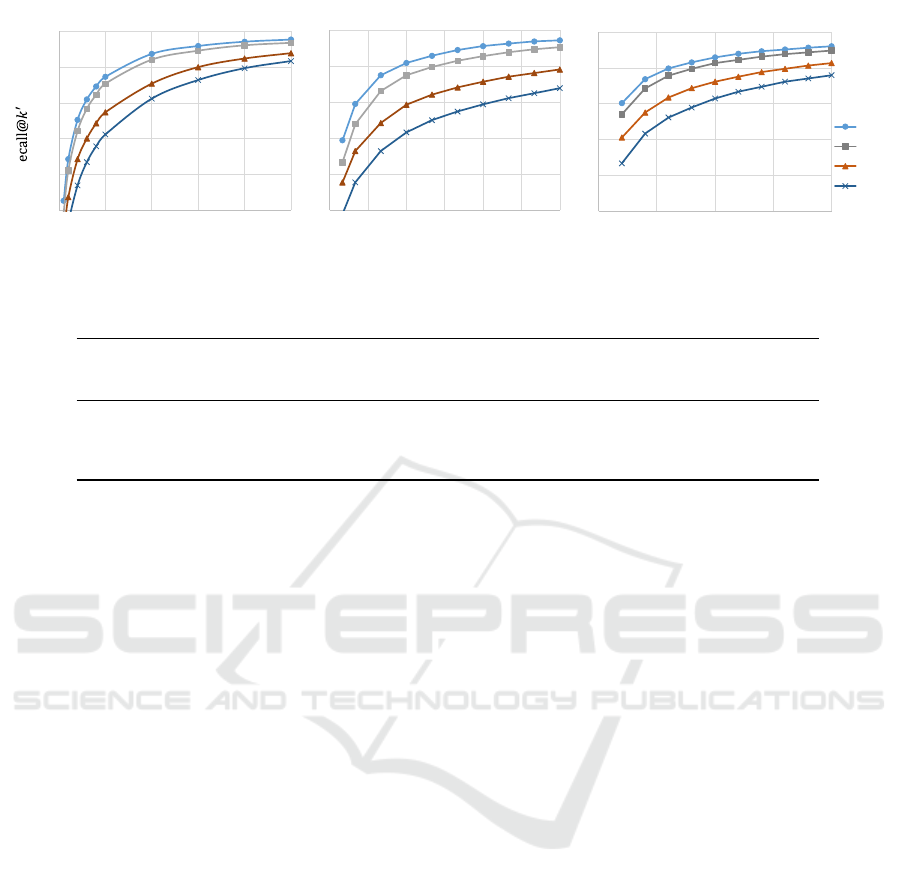
nearest neighbor is included in the candidates.
From Figure 1, it is evident that the filtering
achieves the highest accuracy when prioritizing
e
D
1
and the lowest accuracy when using Hamming dis-
tance, regardless of the dataset. Furthermore, we ob-
serve that even in the case of enumeration based on
Hamming distance, considering the lower bound of
the distance from the query results in better accuracy.
Notably, the accuracy achieved by utilizing conjunc-
tive enumeration closely approaches that of
e
D
1
.
4.4 Closeness to Enumeration in
e
D
1
Order
Figure 1 shows that using conjunctive enumeration re-
sults in filtering performance that is almost as precise
as the enumeration in
e
D
1
order. This is evident in the
similarity between the two enumeration methods. To
quantify the closeness of the enumeration, we employ
a measure based on the ratio of common parts among
an equal number of candidates. Table 5 presents the
recall rates and approximation values for filtering ob-
tained via the other three enumeration methods, con-
sidering the number of candidates where the recall
rate exceeds 90% in
e
D
1
-ordered enumeration for each
dataset. Based on this table, it is evident that for any
dataset, the accuracy and approximation follow the
order: H < H
idx
< Conj..
4.5 Comparison of Filtering Cost
To compare the filtering costs, we examined the case
of the conventional
e
D
1
-ordered enumeration method
and the proposed conjunctive enumeration method.
We adjusted the number of candidates to achieve re-
call rates of 80% and 90% and measured the compu-
tation time required for filtering in each method.
The results are presented in Table 6. For instance,
in the case of the YFCC100M dataset, filtering us-
ing
e
D
1
-ordered enumeration achieves recall rates of
80% and 90% with candidate counts of 0.58 and 1.3
million, respectively, using single-thread serial com-
putation. In the conjunctive enumeration method, the
recall rate tends to decrease with an increasing num-
ber of threads, even with an equal number of can-
didates. To measure the cost for different numbers
of threads, we used the number of candidates for re-
call rates 80% and 90% with 16 threads. For the
Fast Filtering for Similarity Search Using Conjunctive Enumeration of Sketches in Order of Hamming Distance
507

50
60
70
80
90
100
0 1 2 3 4 5
50
60
70
80
90
100
0 3 6 9 12 15 18
50
60
70
80
90
100
0 0.5 1 1.5 2



Conj.



YFCC100M DEEP1B LAION100M
number of candidates 

 




 




 


r
(%)
Figure 1: Comparison of accuracy.
Table 5: Closeness of enumeration to
e
D
1
order.
dataset
k
′
e
D
1
H H
idx
Conj.
(×10
5
) recall recall ∩
e
D
1
recall ∩
e
D
1
recall ∩
e
D
1
YFCC100M 20 94% 81% 55% 85% 64% 92% 80%
DEEP1B 6 91% 72% 42% 79% 55% 88% 75%
LAION100M 8 92% 76% 45% 84% 58% 90% 80%
YFCC100M dataset, the number of candidates for the
conjunctive enumeration method with recall rates of
80% and 90% was set to 0.70 and 1.8 million, respec-
tively.
While filtering with conjunctive enumeration re-
quires slightly more candidates compared to
e
D
1
-
ordered enumeration for all datasets, the accuracy is
comparable. However, even with single-thread serial
processing, the computational cost does not increase
significantly. This observation may be attributed to
the logarithmic delay of the
e
D
1
-ordered enumeration
algorithm relative to the number of enumerations,
while the conjunctive enumeration method exhibits
fast and constant delay. The conjunctive enumera-
tion method demonstrates the potential for speeding
up through parallel processing.
4.6 Total Search Cost
In the previous subsection, we illustrated that the pro-
posed conjunctive enumeration method offers a sig-
nificant reduction in filtering cost compared to the
conventional approach. Nevertheless, beyond the fil-
tering cost, the computational cost of selecting the NN
from filtered candidates plays a crucial role in deter-
mining the overall cost of the NN search. In conjunc-
tive enumeration, to achieve the same recall rate as the
e
D
1
-order enumeration, there is a need to increase the
number of candidates. However, the advantage is that
the filtering cost can be quickly reduced using multi-
thread parallel processing. Note that the cost of NN
selection after filtering increases with the number of
candidates, potentially impacting the efficiency of the
proposed method.
For instance, consider a search with a recall rate
of 80% for the DEEP1B dataset. In the conventional
e
D
1
-order enumeration method, the number of candi-
dates is 2.1 × 10
5
, and filtering takes 0.63 millisec-
onds per query. In contrast, using 16-thread par-
allel processing in the proposed method, the num-
ber of candidates increases to 3.2 × 10
5
, and filter-
ing takes 0.18 milliseconds. For the proposed method
to complete the entire search in less time than the
conventional method, the difference in computation
time for selecting the NN from the candidates must
be less than 0.63 − 0.18 = 0.45 milliseconds. How-
ever, in our experiment environment, the scanning
speed for the NN search in DEEP1B on RAM was 4
nanoseconds per point (using sequential read) and 19
nanoseconds (using random read) when parallel pro-
cessing was performed with 16 threads. Given the
candidate number difference of 1.1 × 10
5
, the com-
putational time difference is magnified by the scan-
ning speed. Even with sequential read, it would take
4 × 10
−9
×1.1 ×10
5
×10
3
= 0.44 milliseconds, indi-
cating that the conventional method and the proposed
method have almost the same search cost. Since
YFCC100M and LAION100M have higher dimen-
sionality compared to DEEP1B, the scanning speed
of the NN search on RAM is slower, which suggests
that the proposed method may have a higher search
cost than the conventional method. Moreover, for
high-dimensional massive datasets like YFCC100M,
it is not practical to load feature data into RAM. This
requires storing feature data on secondary storage,
which in turn, further slows down the process.
ICPRAM 2024 - 13th International Conference on Pattern Recognition Applications and Methods
508

Table 6: Comparison of filtering cost.
1-THD = single-thread, n-THD = n-thread process
dataset recall
e
D
1
conjunctive enumeration
k
′
1-THD k
′
1-THD 2-THD 4-THD 8-THD 16-THD
(×10
6
) (ms/q) (×10
6
) (ms/q) (ms/q) (ms/q) (ms/q) (ms/q)
YFCC100M
80% 0.58 2.5 0.70 1.9 1.4 0.82 0.59 0.51
90% 1.3 6.5 1.8 5.4 3.4 2.2 1.5 1.3
DEEP1B
80% 0.21 0.63 0.32 0.68 0.49 0.34 0.22 0.18
90% 0.55 1.7 0.85 1.9 1.3 0.80 0.55 0.45
LAION100M
80% 0.20 0.52 0.29 0.57 0.42 0.27 0.19 0.16
90% 0.61 1.6 0.87 1.8 1.1 0.68 0.51 0.42
We are currently exploring the method of double
filtering, which involves filtering the narrow-width
sketch’s filtering result using a wider-width sketch or
other projection data. The second filtering stage re-
quires a more compact projection image than the fea-
ture data, with a higher scanning speed and accuracy.
Although it is still in the preliminary experimenta-
tion stage, we have observed that the search speed
can be improved through double filtering, utilizing the
conjunctive enumeration method of the proposed ap-
proach in the first filtering stage. We will provide a
detailed report on this result shortly.
5 CONCLUSION
Although the filtering method proposed in this pa-
per utilizes relatively narrow sketches, it can reduce
the number of candidates to a mere 0.85 million for
DEEP1B when the recall rate is 90%, which is less
than 1/1000 of the dataset size, at a minimal cost.
However, in its current state, the selection in the sec-
ond stage to identify the NN from the candidates is
expensive, making the overall search process not as
rapid. For very large datasets like DEEP1B, it’s fea-
sible to narrow down the candidates with minimal ex-
pense. Hence, rather than using the filtering results
directly for the second-stage search, we can employ
additional filtering to further refine the candidate list.
By using the method of double filtering, we believe
that high-speed and high-precision searches can be
achieved. Though still in the preliminary experimen-
tal phase, when using double filtering, we observed
that the entire search process takes approximately 9.5,
1.4, and 1.8 milliseconds per query for YFCC100M,
DEEP1B, and LAION100M, respectively, at an 80%
recall rate. We will report details of double filtering
shortly.
Unfortunately, it is very difficult to compare the
performance of the filtering proposed in this pa-
per with other studies. At NeurIPS’21 (Simhadri
et al., 2022), a competition was held as “Chal-
lenge on Billion-Scale Approximate Nearest Neigh-
bor Search.” There it competes for filtering-only per-
formance until candidates are selected by an index.
Our filtering method corresponds to Track 1 of the in-
memory index. The applicable conditions for Track
1 are a recall@10 of 65% or higher and a speed
of 10,000 QPS (queries per second) or higher. Re-
call@10 is the recall rate when the number of can-
didates is 10. For DEEP1B, the best record by the
winner is recall@10 = 72% with 10,000 QPS. Our
method takes online search speed into account, so
we think 1,000 QPS is not slow. Double filtering
using our conjunctive filtering runs at recall@10 =
78% in 1 millisecond (1,000 QPS) for DEEP1B. For
LAION100M, it runs at recall@10 = 72% in 1 mil-
lisecond. Empirically, YFCC100M has 4,096 dimen-
sions, so it has only one-tenth the number of points of
DEEP1B, but the search process is more difficult than
DEEP1B. YFCC100M was not used in the competi-
tion. From these facts, it can be said that the proposed
method is very good as an approximation index.
In this paper, the conjunctive enumeration ap-
proach utilizes common low-add combinations for all
queries. In practice, the optimal low-add combination
probably differs for each query. Future work will in-
volve developing a method to select the optimal com-
bination for a given query and further enhancing the
accuracy and speed of the filtering process.
ACKNOWLEDGEMENTS
This research was partially supported by the Japan
Society for the Promotion of Science (JSPS) through
KAKENHI grants numbered 23H03461, 19K12125,
20H05962, 19H01133, 21H03559, and 20K20509, as
well as by a research grant (VIL50110) from VIL-
LUM FONDEN.
Fast Filtering for Similarity Search Using Conjunctive Enumeration of Sketches in Order of Hamming Distance
509

REFERENCES
Amato, G., Falchi, F., Gennaro, C., and Rabitti, F. (2016).
YFCC100M-HNfc6: A large-scale deep features
benchmark for similarity search. In Proc. SISAP’16,
LNCS 9939, Springer, pages 196–209.
Babenko, A. and Lempitsky, V. (2016). Efficient indexing
of billion-scale datasets of deep descriptors. In Proc.
CVPR’16, IEEE Computer Society, pages 2055–2063.
Ciaccia, P., Patella, M., and Zezula, P. (1997). M-tree: An
efficient access method for similarity search in metric
spaces. In Proc. VLBD’97, pages 426–435.
Dong, W., Charikar, M., and Li, K. (2008). Asymmetric
distance estimation with sketches for similarity search
in high-dimensional spaces. In Proc. ACM SIGIR’08,
pages 123–130.
Guttman, A. (1984). R-trees: A dynamic index structure
for spatial searching. In Yormark, B., editor, Proc.
SIGMOD’84, pages 47–57.
Higuchi, N., Imamura, Y., Kuboyama, T., Hirata, K., and
Shinohara, T. (2018). Nearest neighbor search using
sketches as quantized images of dimension reduction.
In Proc. ICPRAM’18, pages 356–363.
Higuchi, N., Imamura, Y., Kuboyama, T., Hirata, K.,
and Shinohara, T. (2019a). Fast filtering for nearest
neighbor search by sketch enumeration without using
matching. In Proc. AusAI’19, LNCS 11919, Springer,
pages 240–252.
Higuchi, N., Imamura, Y., Kuboyama, T., Hirata, K., and
Shinohara, T. (2019b). Fast nearest neighbor search
with narrow 16-bit sketch. In Proc. ICPRAM’19,
pages 540–547.
Higuchi, N., Imamura, Y., Kuboyama, T., Hirata, K., and
Shinohara, T. (2020). Annealing by increasing re-
sampling. In Revised Selected Papers, ICPRAM 2019,
LNCS 11996, Springer, pages 71–92.
Higuchi, N., Imamura, Y., Mic, V., Shinohara, T., Hi-
rata, K., and Kuboyama, T. (2022). Nearest-neighbor
search from large datasets using narrow sketches. In
Proc. ICPRAM’22, pages 401–410.
Imamura, Y., Higuchi, N., Kuboyama, T., Hirata, K., and
Shinohara, T. (2017). Pivot selection for dimension
reduction using annealing by increasing resampling.
In Proc. LWDA’17, pages 15–24.
Lv, Q., Josephson, W., Wang, Z., and and K. Li, M. C.
(2006). Efficient filtering with sketches in the ferret
toolkit. In Proc. MIR’06, pages 279–288.
Mic, V., Novak, D., and Zezula, P. (2015). Improving
sketches for similarity search. In Proc. MEMICS’15,
pages 45–57.
Mic, V., Novak, D., and Zezula, P. (2016). Speeding up sim-
ilarity search by sketches. In Proc. SISAP’16, pages
250–258.
M
¨
uller, A. and Shinohara, T. (2009). Efficient similarity
search by reducing i/o with compressed sketches. In
Proc. SISAP’09, pages 30–38.
Schuhmann, C., Beaumont, R., Vencu, R., Gordon, C.,
Wightman, R., Cherti, M., and Jitsev, . J. (2022).
LAION-5B: An open large-scale dataset for training
next generation image-text models. In arXiv preprint
arXiv:2210.08402.
Shinohara, T. and Ishizaka, H. (2002). On dimension re-
duction mappings for approximate retrieval of multi-
dimensional data. In Progress of Discovery Science,
LNCS 2281, Springer, pages 89–94.
Simhadri, H. V., Williams, G., Aum
¨
uller, M., Douze, M.,
Babenko, A., Baranchuk, D., Chen, Q., Hosseini, L.,
Krishnaswamy, R., Srinivasa, G., Subramanya, S. J.,
and Wang, J. (2022). Results of the NeurIPS’21 chal-
lenge on billion-scale approximate nearest neighbor
search. CoRR, abs/2205.03763.
Wang, Z., Dong, W., Josephson, W., Q. Lv, M. C., and Li,
K. (2007). Sizing sketches: A rank-based analysis
for similarity search. In Proc. ACM SIGMETRICS’07,
pages 157–168.
ICPRAM 2024 - 13th International Conference on Pattern Recognition Applications and Methods
510