Estimation of the Inference Quality of Machine Learning Models for

Cutting Tools Inspection

Kacper Marciniak

1 a

, Paweł Majewski

2 b

and Jacek Reiner

1 c

Faculty of Mechanical Engineering, Wrocław University of Science and Technology, Poland

Faculty of Information and Communication Technology, Wrocław University of Science and Technology, Poland

Keywords:

Machine Vision, Machine Learning, Tool Inspection, Tool Measurement, Inference Quality.

Abstract:

The ongoing trend in industry to continuously improve the efﬁciency of production processes is driving the

development of vision-based inspection and measurement systems. With recent signiﬁcant advances in arti-

ﬁcial intelligence, machine learning methods are becoming increasingly applied to these systems. Strict re-

quirements are placed on measurement and control systems regarding accuracy, repeatability, and robustness

against variation in working conditions. Machine learning solutions are often unable to meet these require-

ments - being highly sensitive to the input data variability. Given the depicted difﬁculties, an original method

for estimation of inference quality is proposed. It is based on a feature space analysis and an assessment of the

degree of dissimilarity between the input data and the training set described using explicit metrics proposed

by the authors. The developed solution has been integrated with an existing system for measuring geometric

parameters and determining cutting tool wear, allowing continuous monitoring of the quality of the obtained

results and enabling the system operator to take appropriate action in case of a drop below the adopted thre-

shold values.

1 INTRODUCTION

Machining is a common manufacturing method used

in the industry to produce high-quality machine and

equipment parts where a high degree of dimensional

accuracy is crucial. Cutting tools used in mass pro-

duction degrade rapidly, negatively impacting their

performance in the machining process and the overall

quality of the manufactured product. For this reason,

tools are subjected to reconditioning, which, in the

case of the hob cutters discussed in this article, invo-

lves removing a layer of material from the tooth attack

face in a grinding process. Removing too little mate-

rial will not fully eliminate the defect (leading to im-

proper tool performance), while using too much allo-

wance will signiﬁcantly shorten its life (Gerth, 2012).

Therefore, an accurate assessment of the degree of

wear and the selection of optimal parameters for the

reconditioning method becomes a critical aspect of

reducing remanufacturing costs while increasing tool

life signiﬁcantly.

https://orcid.org/0009-0000-7098-5907

https://orcid.org/0000-0001-5076-9107

https://orcid.org/0000-0003-1662-9762

The conventional approach to solving the problem

of gear hobbing tool wear estimation involves ma-

nual visual inspection of tools, which is highly inef-

ﬁcient and therefore, various innovative approaches

have been proposed, such as analysis of CNC ma-

chine parameters using multilayer perceptron (MLP)

(Wang et al., 2021) or estimation based on data from

numerical simulations (Bouzakis et al., 2001), (Dong

et al., 2016). Our team proposed a solution in the form

of a machine vision system for inspecting the tooth

rake surfaces of hobbing tools, enabling their dimen-

sioning and unambiguous determination of the wear

level of each tool after the production cycle. This sys-

tem is based on machine learning image processing

models, and it is therefore subject to all their limi-

tations, such as a signiﬁcant susceptibility to the va-

riability of the input data character, which negatively

impacts the model’s accuracy (Szegedy et al., 2014),

(Nguyen et al., 2015), (Dalva et al., 2023). This pro-

blem becomes critical when one considers how di-

verse the tools undergoing the scanning process are,

varying in shape, dimensions, or surface quality and

texture. As a solution to this problem, two fully com-

plementary strategies can be proposed: (1) improving

the robustness of the ML model to the variability of

Marciniak, K., Majewski, P. and Reiner, J.

Estimation of the Inference Quality of Machine Learning Models for Cutting Tools Inspection.

DOI: 10.5220/0012321900003660

Paper published under CC license (CC BY-NC-ND 4.0)

In Proceedings of the 19th International Joint Conference on Computer Vision, Imaging and Computer Graphics Theory and Applications (VISIGRAPP 2024) - Volume 3: VISAPP, pages

359-366

ISBN: 978-989-758-679-8; ISSN: 2184-4321

359

the input data, (2) preparing a methodology to esti-

mate the quality of the inference, which would allow

the results to be evaluated and possibly rejected. This

paper focuses on the second solution, based on fe-

ature space analysis methods, as this approach is hi-

ghly versatile and easily applicable to other machine

vision systems.

Analysing the distribution of deep data features

used in machine learning is a process long familiar

to researchers and data engineers. It is widely used

to evaluate data distributions, determine the level of

heterogeneity, and in classiﬁcation tasks (Umbaugh,

2005). The method has recently begun to be utilised

in the label-free evaluation of machine learning mo-

dels. An example is the ’AutoEval’ method (Deng and

Zheng, 2020), which allows indirect determination of

ML model accuracy on a given test set by analysing

differences in the distribution of input and training

data, calculated as Fréchet Inception Distance (FID)

and referred to as distribution shift. Classiﬁcation ac-

curacy is determined using a regression model. The

cited work develops a general methodology that al-

lows application to various models or data and identi-

ﬁes its limitations. Analysis in feature space using the

FID metric is also widely used in the Generative Ad-

versarial Networks (GANs) evaluation process (Bu-

zuti and Thomaz, 2023).

Considering existing research gaps in the form of

a lack of practically applicable solutions for analy-

sing and evaluating machine learning systems under

industrial conditions, work was undertaken to deve-

lop a methodology for the automatic estimation of in-

ference quality of machine learning models. The pro-

posed solution is based on analysing the data distribu-

tion in the deep feature space and allows the level of

inference quality on a given image to be determined

unambiguously. It is worth noting that the proposed

solution has been developed to be implemented and

practically used in a simultaneously developed indu-

strial machine vision system.

2 MATERIALS AND METHODS

2.1 Problem Deﬁnition

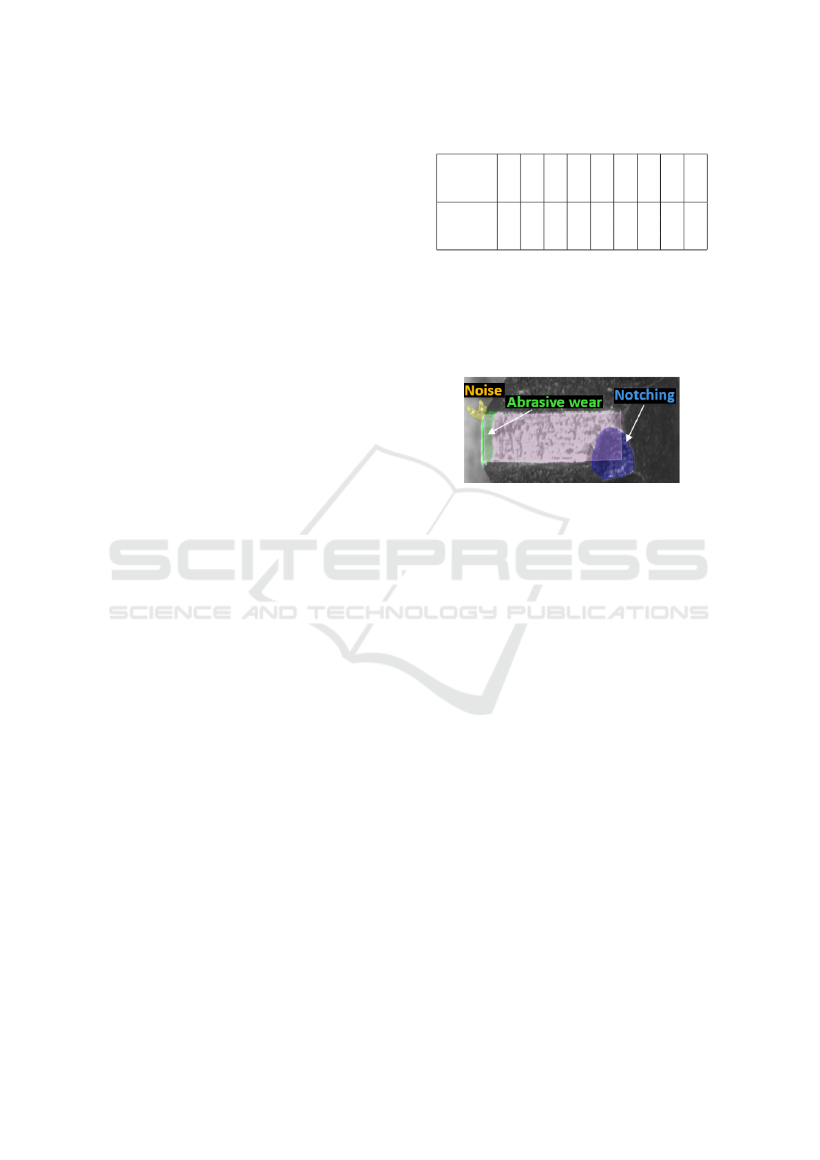
The problem described is the segmentation of tooth

rake faces of cutting tools (hob cutters) to measure

their geometric parameters, as well as the segmen-

tation of defects such as abrasive wear (shallow da-

mage to the surface), notching (deep tooth damage)

and build-up or contamination (Figure 1). This task is

non-trivial because of the signiﬁcant variations of the

data obtained when scanning different tools, which

Table 1: Prepared multi-domain training datasets.

Multi

domain

set

1 2 3 4 5 6 7 8 9

Tools

1 1 3 4 4 5 4 3 3

8 2 6 5 5 6 5 8 7

9 8 9 9 6 7 7 9 9

are due to the following: 1. variations in tool geometry

between the different tool types, 2. different degrees

and ways of wear depending on the working time and

load of the tool, 3. the use of different protective co-

atings on the tools, 4. variable acquisition conditions

resulting from an incorrect scanning process by the

system user.

Figure 1: Examples of typical failures detected on the tooth

rake face.

2.2 Dataset

The dataset was created using raw images of hob teeth

with a dimension of 4024x3036 pixels, from which

regions-of-interest (ROIs) containing tooth rake faces

were cropped. The size of the cropped area was con-

stant for a given tool type, and its values were de-

termined by the nominal tooth length and tool pitch

value.

The prepared dataset contained images of nine

unique tools differing in wear, geometry and coating

used (Figure 2), each containing 50 images with an-

notated rake faces. These sets of tooth images are

referred to in the following paper as sub-domains.

Each set was split in an 80/20 ratio to create inde-

pendent training and test subsets. The study inclu-

ded nine single-domain test datasets containing ap-

proximately ten images of a single tool each and nine

multi-domain training sets with three randomly selec-

ted subdomains (Table 1). This resulted in 9 unique

sets of images and labels for training the test segmen-

tation models and 9 test sets for evaluation.

2.3 Model Preparation

The experiment used Detectron2 implementations of

the FasterRCNN-ResNet101-FPN (Wu et al., 2019)

instance segmentation architecture with PointRend

support (Kirillov et al., 2019). Each of the 19 tra-

VISAPP 2024 - 19th International Conference on Computer Vision Theory and Applications

360

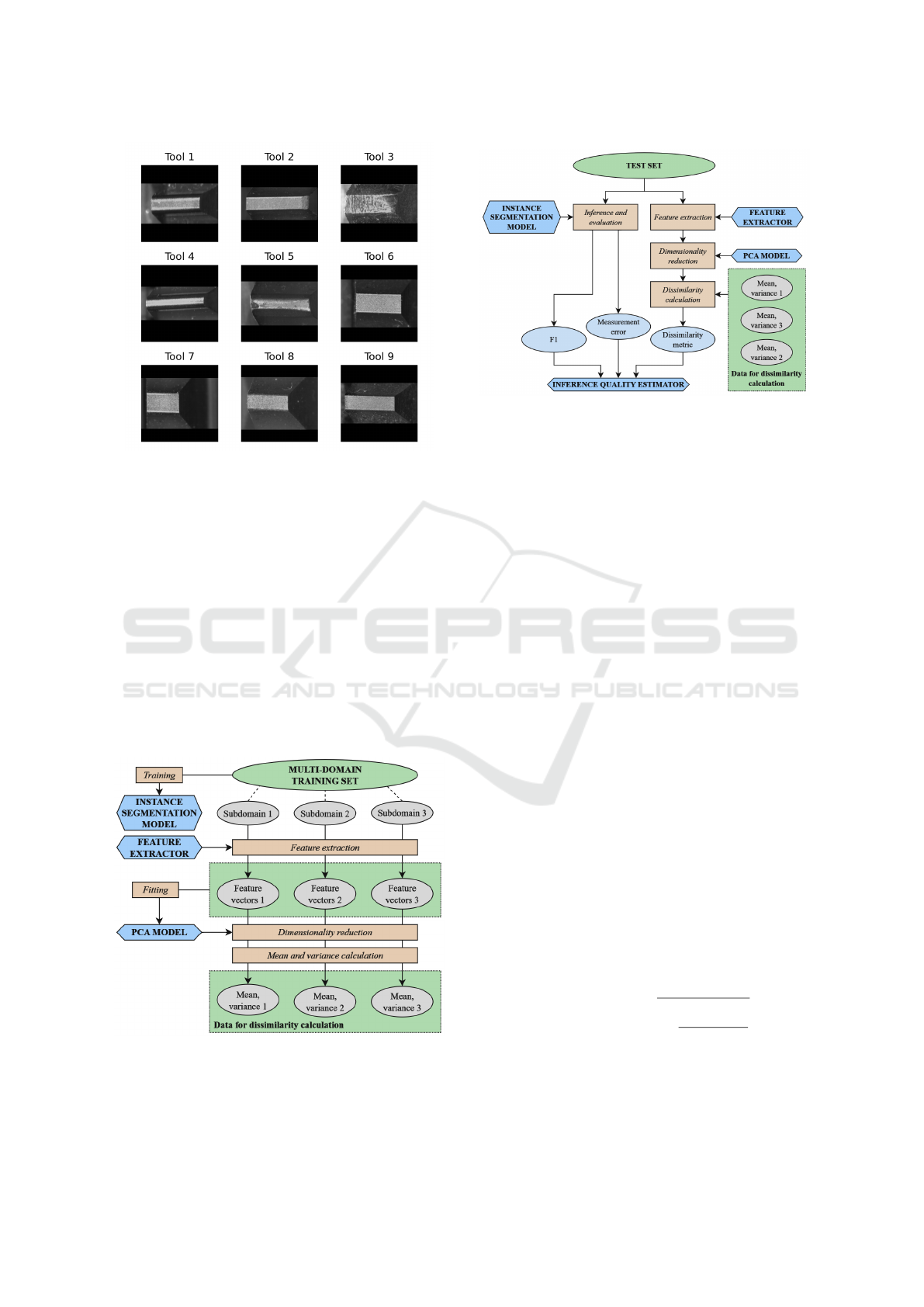
Figure 2: Example images of tools included in the dataset.

ining processes was performed with batch_size = 4

and epochs = 25, except for the ﬁnal model trained on

all subdomain data with a larger epoch number of 35.

The number of epochs was chosen experimentally ba-

sed on the analysis of data from the training process.

2.4 Proposed Method

The experiment proposes a comprehensive processing

pipeline for both single and multi-domain sets (Figure

3), utilised in the preparation of models (instance seg-

mentation, PCA) and data distribution metrics (mean

and variance), which are subsequently used in the de-

velopment of the inference quality estimator (Figure

4).

Figure 3: Proposed pipeline for model training and data ana-

lysis.

Figure 4: Model evaluation and quality estimator prepara-

tion - proposed method.

2.4.1 Feature Extraction

An extractor based on the pre-trained classiﬁcation

model with ResNet-101 architecture (He et al., 2015)

and the ’IMAGENET1K_V2’ set of weights was used

to extract deep features from the images. Before fe-

ature extraction, the images were transformed to a

square shape by padding with black bars and resca-

led to a size of 200x200 pixels. The standard norma-

lisation procedure was applied: mean = [0.485, 0.456,

0.406], std = [0.229, 0.224, 0.225]. The dimensions of

the resulting feature vectors were reduced using Prin-

cipal Component Analysis (PCA). The PCA model

was prepared based on feature vectors related to ima-

ges from training sets from all sub-domains, and the

output dimension was chosen to ensure that at least

99% of the training data variance was maintained.

2.4.2 Determination of the Level of Data

Dissimilarity

The level of dissimilarity between the input image and

reference set was deﬁned as the distance in feature

space between image feature vector F

and data di-

stribution deﬁned by mean µ and covariance σ. The

following metrics were examined:

• Euclidean distance;

• standardised Euclidean distance (1);

• Mahalanobis distance.

D(F

, µ, σ) =

∑

i=1

(µ

− F

)

(1)

Where k is the length of a feature vector.

For models trained on multi-domain sets, two

ways of measuring dissimilarity have been proposed:

Estimation of the Inference Quality of Machine Learning Models for Cutting Tools Inspection

361

1. measuring the distance between the input image fe-

ature vector and the entire data distribution, 2. deter-

mining the distance as a weighted average of the di-

stances of the image feature vector to the subdomains

that form the data set (as explained on Figure 5). The

weighted average is deﬁned as follows (2):

avg

∑

i=1

∗ D(F

, mean(F

), std(F

)) (2)

where N is the number of subdomains and w

is the

weight determined using the average value of the F1

metric (F1

) obtained during the evaluation of the re-

spective subdomain (3):

1.5 − F1

eval

∑

i=1

(1.5 − F1

eval

)

(3)

This approach favours subdomains with a lower F1

value, taking distances to them with more weight

when calculating the dissimilarity metric. d

is the

distance between the i-th subdomain’s image feature

vector.

The proposed metric made it possible to assess the

level of dissimilarity of the input data from the tra-

ining data by determining the weighted average of

the distances to each subdomain while considering

the quality of the model’s inference on the mentioned

subdomains.

Figure 5: Proposed method of calculating distance between

image and multiple subdomains in feature space.

2.4.3 Custom Model Evaluation

A conﬁdence threshold of 0.75 was adopted after ana-

lysing the F1 - conﬁdence score relationship obtained

from the evaluation of the multi-domain model. The

following metrics were proposed to evaluate the mo-

del for a chosen working point:

• pixel-wise F1-score (4) calculated using predic-

tion mask (P) and label mask (L);

• mean of absolute error of rake face width and

length measurement.

F1 =

2 ∗ TP

2 ∗ TP + FP + FN

T P =

∑

(P ∧ L)

∑

FP =

∑

(P∧ ̸ L)

∑

FN =

∑

(̸ P ∧ L)

∑

(4)

Each model was evaluated using images from the

subdomain test sets - raw quality metrics (F1, measu-

rement error) and data dissimilarity were determined.

To assess the quality of the model’s inference as a

function of data dissimilarity, the following metrics

were proposed and tested:

• cumulative average of quality metrics;

• proportion of correct predictions for a given data

dissimilarity threshold;

• squared proportion of correct predictions for a gi-

ven data dissimilarity threshold;

Determination of the proportion of correct pre-

dictions and measurements was carried out for 15

domain distance thresholds and boundary values of

thresh

geo

= 0.050 mm and F

thresh

= 0.90.

2.5 Model Inference Quality Estimator

Preparation

Based on the quality metrics from the model evalu-

ation and the dissimilarity index of the data, the tar-

get estimator should determine the inference quality

in the form of a number between 0 and 1, where 1

indicates the highest quality of the results obtained

and, thus, their highest reliability. The proposed so-

lution involves approximating the relationship of the

quality metrics to the data dissimilarity index with a

mathematical function and using it in the production

process.

2.6 Effect of the Number of New

Samples on the Change in the

Inference Quality

In addition, work was undertaken to determine the

impact of new samples in the training dataset on

the quality of inference by the model. As a result,

a model trained on a multi-domain data set and two

single-domain test sets were selected, for which the

inference quality was substantially lower. For each

model-subdomain test pair, 5, 10, 20 and 40 sam-

ples were randomly selected from the training set of

VISAPP 2024 - 19th International Conference on Computer Vision Theory and Applications

362

the examined subdomain. These samples were used to

supplement the training set and prepare a new model.

The process was repeated ﬁve times, and the results

were averaged. This allowed to plot the dependence

of the inference quality on the subdomain on the num-

ber of corresponding samples from the subdomain in

the training set.

3 RESULTS AND DISCUSSION

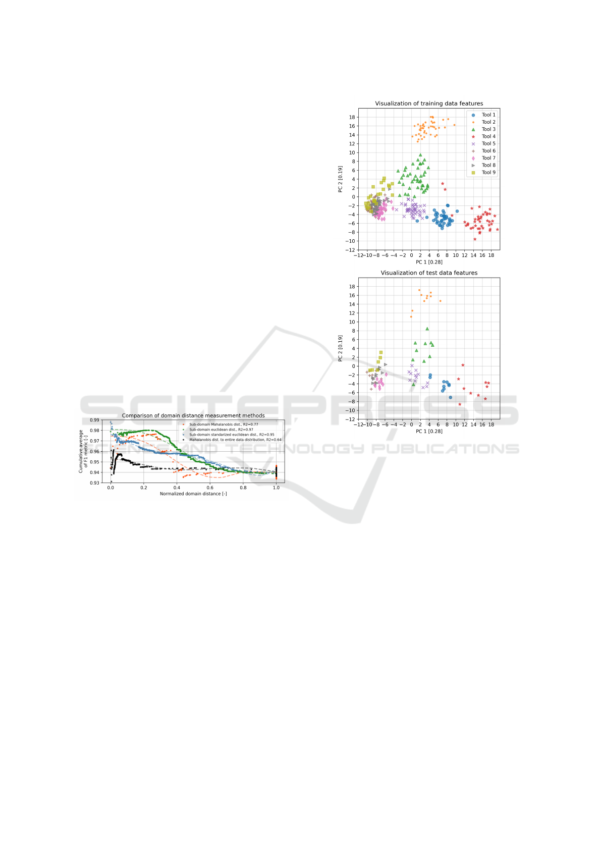
3.1 Data Dissimilarity Calculation

To determine the method for calculating the data dis-

similarity metric, the change in the cumulative ave-

rage of F

value as a function of domain distance

was analysed (Figure 6), and the coefﬁcients of de-

termination for the third-degree polynomial estima-

tion of these runs were determined. Of the analysed

approaches, the Mahalanobis distance determined for

both subdomains and entire data distribution proved

to be the least successful, with a low coefﬁcient of

= 0.77 and R

= 0.64. The method based on the

standardised Euclidean distance with R

= 0.97 and a

shape close to the expected one was the best and was

used in further work.

Figure 6: Comparison of different domain distance measu-

rement methods.

3.2 Inference Quality as a Function of

Domain Distance

All subdomain data from the prepared dataset was put

through a process of feature extraction followed by

dimensionality reduction. The PCA model prepared

reduced the feature vectors from 2048 to 180 dimen-

sions, which resulted in the preservation of 99.004%

of the variance. A graphical visualisation of the distri-

bution of the deep features of the training and test sets

for the ﬁrst two principal components is presented be-

low (Figure 7).

Each of the nine single-domain models, nine

three-domain models and the all-domain model were

evaluated on prepared test sets. The relationships pre-

sented in the graphs below were determined based on

Figure 7: Visualisation of training and eval data features.

the qualitative and dissimilarity metrics obtained. Do-

main distance values ranging from 6.30 to 28.0 and a

median of 12.5 were obtained. Values of the F

me-

tric ranged from 0 (no object detection) to 0.994, with

a median of 0.969. For side face measurement error,

values ranged from 0 to 4.97 mm, with a median of

0.047 mm. The cumulative average of the F

metric

(Figure 8) trended as expected. With an increase in

the difference between the input image and the tra-

ining data set (domain distance), a signiﬁcant decre-

ase in the inference quality metric was observed. It is

worth noting the course of the plots, which were stair-

stepping for some models - large differences in in-

ference quality occurred when transitioning between

test subdomains. The fastest decrease in inference qu-

ality as a function of domain distance was observed

for models prepared using training sets consisting of

images of tools 4, 5 and 6, two of which (tools 4 and

5) are signiﬁcantly similar. At the same time, the lo-

west values were achieved for the high value of do-

main distance for models trained with data from tools

1, 8, 9 and 1, 2, 8.

Estimation of the Inference Quality of Machine Learning Models for Cutting Tools Inspection

363

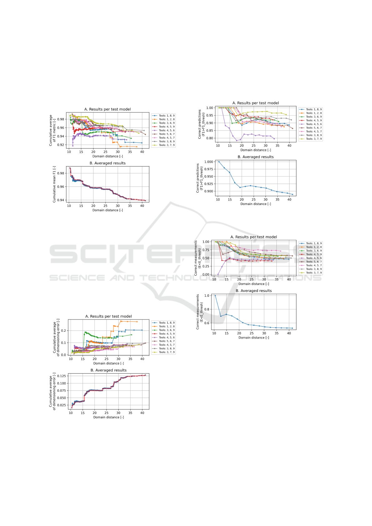
The averaged function took a straight line shape

up to a domain distance value of 20, later plateauing

and holding constant at F

= 0.94. In this evaluation

graph, the red line shows the course of the cumulative

maximum value, which is one of the proposed inputs

to the quality estimator being developed.

Figure 8: Cumulative average of F1 metric in the domain

distance function: A. results per test model, B. averaged re-

sults.

The cumulative average of the tooth rake face di-

mensioning error increases with domain distance, re-

aching values above E

geo

= 0.20 mm for models tra-

ined on tool images 1, 8, 9 and 1, 2, 8. A signiﬁcant

increase in error is also observed for the set that con-

tains similar domains 6 and 9, as well as the charac-

teristic domain 3 (a tool with high wear and unusual

surface texture). The ﬁnal result was an averaged plot

similar to the F

metric, albeit with values increasing

as a function of dissimilarity (Figure 9).

Figure 9: Cumulative average of rake face measurement er-

ror in the domain distance function: A. results per test mo-

del, B. averaged results.

When analysing the number of correct predictions

and measurements, the lowest prediction performance

was recorded for the model trained on sets 4, 5, 6,

whilst the lowest measurement performance was ob-

served with 4, 5, 9 (Figures 10 and 11).

Figure 10: Proportion of correct predictions for given do-

main distance thresholds: A. results per test model, B. ave-

raged results.

Figure 11: Proportion of correct measurements for given do-

main distance thresholds: A. results per test model, B. ave-

raged results.

Any anomalies and deviations in the presented re-

sults may be due to the proposed method of deter-

mining differences between the image and input data

(domain distance). Developing a metric that would

unambiguously relate the differences between the di-

stributions of deep data features and the quality of in-

ference by the deep model is a non-trivial task. It re-

quires further work and testing, including testing on

new data sets and using other feature extractors, for

example, based on our classiﬁcation models.

VISAPP 2024 - 19th International Conference on Computer Vision Theory and Applications

364

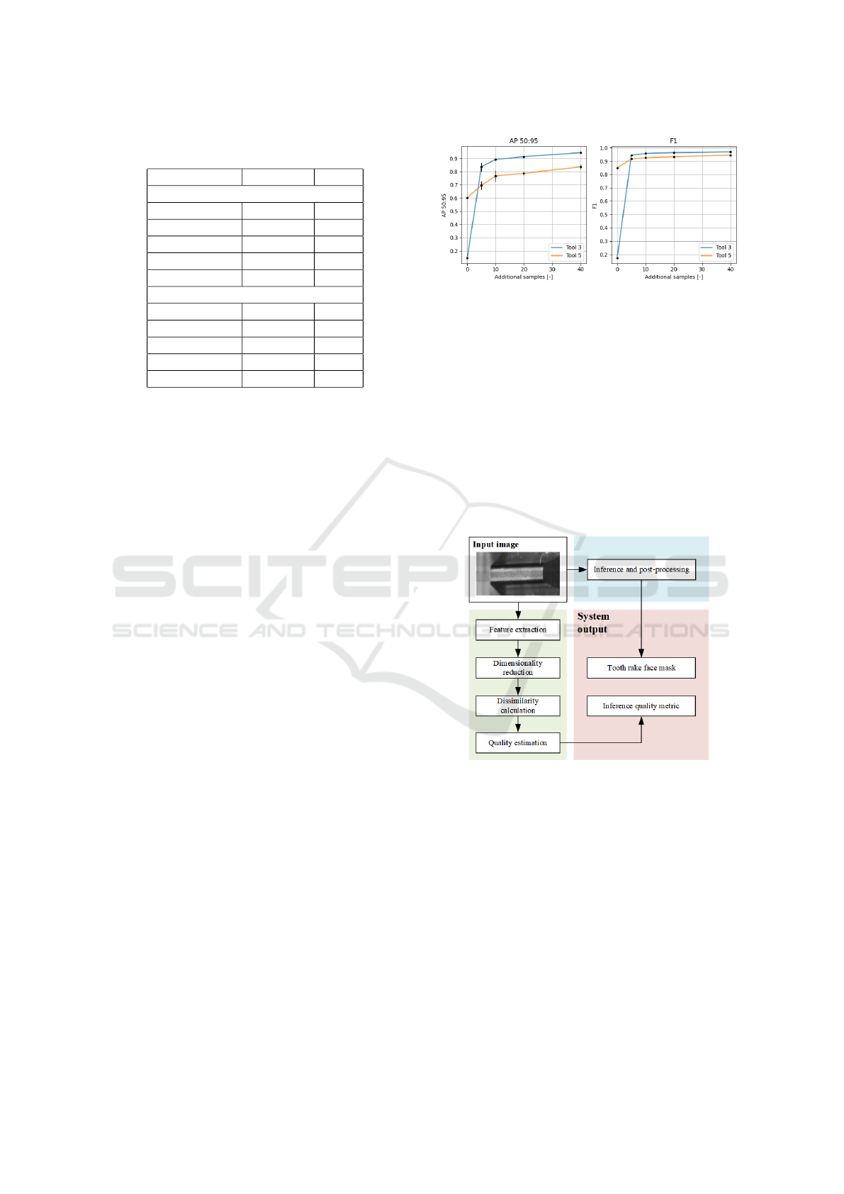
Table 2: Effect of the number of new samples on the change

in the inference quality.

New samples AP 50:95 F1

Tool 2

0 0.146 0.173

5 0.836 0.945

10 0.893 0.958

20 0.913 0.963

40 0.943 0.968

Tool 4

0 0.603 0.849

5 0.696 0.917

10 0.767 0.925

20 0.786 0.933

40 0.836 0.945

3.3 Effect of the Number of New

Samples on the Change in the

Inference Quality

The model selected for the study was trained on a

multidomain built from images of tools 1, 2 and 8.

Images of tools 3 and 5 with inference on which the

model had problems were used as test samples. In

both cases, similar results were observed - the shar-

pest, steepest change in the quality of inference oc-

curred when the ﬁrst samples were added - for tool 2

it was a change in AP

50:95

from 0.146 to 0.83 and F

from 0.173 to 0.945 after adding ﬁve samples (11.9%

of the available set), for tool 4: a change in AP

50:95

from 0.603 d 0.767 and F

from 0.849 to 0.917 for

ten samples (21.3%), with subsequent changes in qu-

ality for both tools being much smaller (Table 2). The

data obtained suggest that even a few samples (10)

from a given domain can signiﬁcantly improve the in-

ference quality of the machine learning (ML) model.

This knowledge can be used to automate the inference

quality control process, where when a large difference

is detected between the input data set and the training

set, the system will perform a feature analysis and se-

lect a sample set for labelling, the size of which will

ensure an improvement in the quality of the model’s

work while minimising the amount of time and effort

to process and prepare the selected training data.

3.4 Integration with the Machine Vision

Inspection System

The proposed methodology has been integrated into a

developed system for cutting tool inspection. During

the inference process, each input image is compared

with the training set of the model used and the degree

of dissimilarity is determined. This value is used to es-

Figure 12: Experiment results for tools 2 and 4.

timate the expected level of inference quality (Figure

13). This information is communicated to the user and

allows an assessment of the level of reliability of the

results obtained so that appropriate action can be ta-

ken:

• accept the results obtained and use them to decide

on the tool regeneration method,

• ignore or modify the results with a low level of

reliability,

• stop the system and select additional training sam-

ples to prepare a new model - in the case of a cri-

tically low level of reliability.

Figure 13: Conceptual scheme of the inference process.

4 CONCLUSIONS

The results presented in this paper showed the possi-

bility of correlating the degree of dissimilarity of the

input and training data in feature space with the infe-

rence quality metrics of the machine learning model.

This demonstrates the potential of using this appro-

ach to estimate the performance quality of ML-based

machine vision systems in production environments.

Such a solution is very much needed for systems with

high input data variability. An example would be cut-

ting tool wear assessment equipment, where the re-

sults’ quality can be signiﬁcantly and negatively af-

Estimation of the Inference Quality of Machine Learning Models for Cutting Tools Inspection

365

fected every time the tool parameters change. A sys-

tem based on the proposed methodology would allow

not only the assessment of the reliability of inference

results but also the automation of the process of tra-

ining data selection by indicating the optimal number

of samples needed.

The machine learning models deployed as part of

this experiment respond differently to the variability

of the deep features extracted from input images, sho-

wing high robustness even to signiﬁcant changes in

some of them while simultaneously being highly sen-

sitive to others. For this reason, further work would

be required to improve the proposed methodology for

determining the degree of dissimilarity of the data by

developing methods that are less general and closely

related to the character of the processed data. The con-

sidered approaches are the use of feature extractors

based on image classiﬁers trained on images of cut-

ting tools acquired with the developed vision system

or direct determination of inference quality with the

use of a regression model.

ACKNOWLEDGEMENTS

We want to thank Wojciech Szel ˛ag and Mariusz

Mrzygłod from the Wrocław University of Techno-

logy, who took an active part in the development and

construction of the machine vision system used, as

well as the staff at TCM Poland for providing the ma-

terials necessary to carry out the work described in

this paper.

REFERENCES

Bouzakis, K.-D., Kombogiannis, S., Antoniadis, A., and

Vidakis, N. (2001). Gear Hobbing Cutting Pro-

cess Simulation and Tool Wear Prediction Models .

Journal of Manufacturing Science and Engineering,

124(1):42–51.

Buzuti, L. F. and Thomaz, C. E. (2023). Fréchet autoen-

coder distance: A new approach for evaluation of ge-

nerative adversarial networks. Computer Vision and

Image Understanding, 235:103768.

Dalva, Y., Pehlivan, H., Altındi¸s, S. F., and Dundar, A.

(2023). Benchmarking the robustness of instance seg-

mentation models. IEEE Transactions on Neural Ne-

tworks and Learning Systems, pages 1–15.

Deng, W. and Zheng, L. (2020). Are labels neces-

sary for classiﬁer accuracy evaluation? CoRR,

abs/2007.02915.

Dong, X., Liao, C., Shin, Y., and Zhang, H. (2016). Ma-

chinability improvement of gear hobbing via process

simulation and tool wear predictions - the internatio-

nal journal of advanced manufacturing technology.

Gerth, J. L. (2012). Tribology at the cutting edge: a study

of material transfer and damage mechanisms in metal

cutting. PhD thesis, Acta Universitatis Upsaliensis.

He, K., Zhang, X., Ren, S., and Sun, J. (2015). Deep resi-

dual learning for image recognition.

Kirillov, A., Wu, Y., He, K., and Girshick, R. (2019). Poin-

tRend: Image segmentation as rendering.

Nguyen, A., Yosinski, J., and Clune, J. (2015). Deep neural

networks are easily fooled: High conﬁdence predic-

tions for unrecognizable images. In Proceedings of

the IEEE Conference on Computer Vision and Pattern

Recognition (CVPR).

Szegedy, C., Zaremba, W., Sutskever, I., Bruna, J., Erhan,

D., Goodfellow, I., and Fergus, R. (2014). Intriguing

properties of neural networks.

Umbaugh, S. (2005). Computer Imaging: Digital Image

Analysis and Processing. A CRC Press book. Taylor

& Francis.

Wang, D., Hong, R., and Lin, X. (2021). A method for

predicting hobbing tool wear based on cnc real-time

monitoring data and deep learning. Precision Engine-

ering, 72:847–857.

Wu, Y., Kirillov, A., Massa, F., Lo, W.-Y., and Gir-

shick, R. (2019). Detectron2. https://github.com/

facebookresearch/detectron2.

VISAPP 2024 - 19th International Conference on Computer Vision Theory and Applications

366