GNNDLD: Graph Neural Network with Directional Label Distribution

Chandramani Chaudhary

, Nirmal Kumar Boran

, N Sangeeth

and Virendra Singh

National Institute of Technology Calicut, Kozhikode, India

National Institute of Technology, Trichy, Tiruchirappalli, India

Indian Institute of Technology Bombay, Mumbai, India

Keywords:

Graph Neural Network, Heterophily, Homophily, Oversmoothing, Decoupling.

Abstract:

By leveraging graph structure, Graph Neural Networks (GNN) have emerged as a useful model for graph-based

datasets. While it is widely assumed that GNNs outperform basic neural networks, recent research shows that

for some datasets, neural networks outperform GNNs. Heterophily is one of the primary causes of GNN

performance degradation, and many models have been proposed to handle it. Furthermore, some intrinsic

information in graph structure is often overlooked, such as edge direction. In this work, we propose GNNDLD,

a model which exploits the edge direction and label distribution around a node in varying neighborhoods

(hop-wise). We combine features from all layers to retain both low-pass frequency and high-pass frequency

components of a node because different layers of neural networks provide different types of information. In

addition, to avoid oversmoothing, we decouple the node feature aggregation and transformation operations.

By combining all of these concepts, we present a simple yet very efﬁcient model. Experiments on six standard

real-world datasets show the superiority of GNNDLD over the state-of-the-art models in both homophily and

heterophily.

1 INTRODUCTION

In many domains, including biological, chemical, so-

cial, etc., data can be naturally modeled as graphs

forming cell or gene graphs, molecular structures, so-

cial networks, and so on. Graphs are powerful data

representations, however, they can not be represented

in Euclidean space. Due to this, traditional machine

learning models are unable to model them. Deal-

ing with graph data presents several issues, including

how to represent or use the structural information of a

graph and how to utilize neighborhoods with no order

and no ﬁxed size. Many existing (Zhu et al., 2020;

Grover and Leskovec, 2016; Hu et al., 2021) sta-

tistical models consider ordered and ﬁxed-size input

for graph data, which cannot capture all information

and may include noise by considering order among

nodes. The Graph Neural Network (GNN) (Scarselli

et al., 2009) is the most recent state-of-the-art (SOTA)

model leveraging machine learning methodologies on

graphs to address these problems. In GNNs, the struc-

tural information is incorporated with the graph enti-

ties, such as node features and/or edge features and/or

labels, etc. Similar to CNNs (Yao et al., 2019), GNNs

can recursively gather information from neighboring

nodes in the graph, which includes both spatial and

node features.

Although GNNs have improved numerous tasks,

the majority of GNN-based models consider the graph

as a homophilous graph (homophily). A network with

the homophily property states that similar nodes are

more likely to attach to one other than dissimilar ones.

Since the majority of real-world networks contain a

variety of nodes and edges, such assumptions are un-

realistic. In a citation network, for example, there

are different node types, such as paper, author, area,

and so on, as well as edges between different types of

nodes. These graphs are referred to as heterophilous

networks (heterophily). Due to the extensive and var-

ied information contained in these graphs, the major-

ity of GNN models are unable to comprehend the het-

erophily aspect of the graph. Many models have been

proposed that are spectral-based and design high-pass

ﬁlters to handle heterophily (Luan et al., 2022; Poiitis

et al., 2022). Some methods (Veli

ckovi

c et al., 2018;

Peng et al., 2021) focus on the selection of neighbors

for aggregation function. These methods tend to have

a higher number of parameters than the usual GNN

and hence require more training time. Some methods

(Zhu et al., 2021; Zhong et al., 2022) learn a com-

Chaudhary, C., Boran, N., Sangeeth, N. and Singh, V.

GNNDLD: Graph Neural Network with Directional Label Distribution.

DOI: 10.5220/0012321400003636

Paper published under CC license (CC BY-NC-ND 4.0)

In Proceedings of the 16th International Conference on Agents and Artiﬁcial Intelligence (ICAART 2024) - Volume 2, pages 165-176

ISBN: 978-989-758-680-4; ISSN: 2184-433X

165

patibility matrix to consider label-to-label relations.

In our research, we explore the node-to-label infor-

mation for each node concerning each neighborhood

hop/layer, terming it as label distribution. This refers

to the details regarding which labels are assigned to

the neighboring nodes. This can give a more robust

and local view of label distribution around a node

type instead of considering a generalized compatibil-

ity matrix for all labels, which gives global informa-

tion.

For node classiﬁcation in graphs, some methods

are based on label propagation (LP), which incorpo-

rates label information (Wang and Leskovec, 2020;

Wang and Leskovec, 2021). Typically, LP-based

methods propagate the label information along the

edges and aggregate it at the nodes. In the proposed

work, the distribution of labels is considered for each

node as its feature, unlike in LP. Our work describes

the type of neighborhood around a node, this dis-

tribution aids the proposed model’s ability to deter-

mine whether the graph is more heterophilous or ho-

mophilous.

Some of the existing methods (Fu et al., 2020)

try to improve the embeddings of graphs with metap-

aths. A metapath is an ordered sequence of the net-

work node and edge types that identify a compos-

ite relation between the node types involved. Since

metapath-based models do not consider the rich node

features, they do not perform well on heterophilous

graphs. In the proposed work, we consider the feature

of nodes with directional information. The directional

label distribution considered is with respect to label

distribution around a node, i.e., we use the distribution

of labels among outdegree nodes and indegree nodes

individually. The nodes which share similar types of

directional label distribution tend to be in the same

class.

We propose a novel GNN model where both

homophilous and heterophilous graphs are consid-

ered. To accommodate the properties of both types

of graphs, we design the model to consider aggre-

gated neighborhood features that are typically consid-

ered in the case of homophilous graphs. To improve

upon heterophily issues, we propose to use directional

label distribution features. So, the model not only

uses structural information for generating node fea-

tures from neighbors but also for generating label in-

formation from its neighbors. It has been observed

that as the number of layers (depth) of the model

grows, the node representation degrades (Liu et al.,

2020). There can be two reasons for this: 1) over-

smoothing of node representation- this is more promi-

nent in the case of small graphs, and 2) noise inclu-

sion in node representation- this is more prominent

in large graphs. To overcome oversmoothing, we de-

couple the aggregation and propagation operations of

GNN. Further, to overcome the noise inclusion prob-

lem, we take each individual layer’s features (Skip

Connection (He et al., 2016)). These features are then

combined with initial features to feed them to a fully

connected layer, which is the ﬁnal layer. As a result of

neighborhood node features and directional label dis-

tribution, our proposed model improves the expressiv-

ity of structural and semantic information in graphs.

In our proposed work, we are considering the feature

of nodes with incoming edge directions in neighbor-

hood message aggregation. If we add outgoing node

features, it may deviate from the performance of the

model. This can be handled by a graph attention net-

work (GAT) (Veli

ckovi

c et al., 2018), and we would

like to look into this further in our future work by in-

cluding the edge direction of the edge feature vector.

The edge feature, which requires a lot of processing

resources, is not used in this paper.

In summary, this work makes the following major

contributions:

1) We propose a novel GNN for node classiﬁ-

cation that considers both the homophily and het-

erophily properties of graphs.

2) We design the node representation by reﬂect-

ing the node features, label distribution, and edge di-

rection information. This representation uses differ-

ent powers of the adjacency matrix depending on the

GNN layer.

3) We carry out in-depth experiments to assess the

effectiveness of our proposed approach on three ho-

mophilous graph datasets and six heterophilous graph

datasets for node classiﬁcation. Experiments show

that our method consistently outperforms other state-

of-the-art models and baselines in the classiﬁcation of

nodes in most datasets.

2 RELATED WORK

2.1 Traditional Graph Neural Networks

To improve graph-based tasks GNN is becoming

widely attractive due to its ability to learn from end

to end. Defferrad et al. (Defferrard et al., 2016)

proposed the early GNN model, which discussed

how convolutional neural networks can be general-

ized for graph-based data. Kipf et al. (Kipf and

Welling, 2017) further improved and simpliﬁed the

GNN model with an approximation, which is now the

typical GNN baseline called the graph convolutional

neural network (GCN). Due to the success of attention

models in other deep learning areas, Velickovic et al.

ICAART 2024 - 16th International Conference on Agents and Artiﬁcial Intelligence

166

(Veli

ckovi

c et al., 2018) proposed a graph attention

network to improve neighborhood aggregation.

2.2 Oversmoothing

Many studies show that oversmoothing occurs in

GCN with numerous layers, which causes the repre-

sentation of nodes in each connected component to

converge to an identical representation. This is a re-

sult of aggregate and transformation processes being

used repeatedly (Yan et al., 2022). Li et al. (Li et al.,

2018) work is the ﬁrst study regarding oversmooth-

ing in GCN. The propagation process, according to

the authors, is a unique symmetric type of Laplacian

smoothing that results in a comparable representa-

tion for nodes belonging to the same class. Liu et al.

(Liu et al., 2020) analyze the same problem and pro-

pose adaptive, structure-aware node representations.

To prevent oversmoothing in GNNs with fewer lay-

ers, authors have talked about decoupling the propa-

gation and transformation operations. To overcome

oversmoothing several empirical solutions are pro-

posed such as residual connections (Li et al., 2019),

skip links (Xu et al., 2018), edge dropout (Rong

et al., 2020), new normalization strategies (Zhao and

Akoglu, 2019), etc.

2.3 Heterophily

The crucial issue of heterophily for GNNs was ﬁrst

explored in (Pei et al., 2020). Although MixHop

(Abu-El-Haija et al., 2019) does not speciﬁcally ad-

dress the heterophily issue, it does mention the chal-

lenge of learning in heterophilous graphs and suggests

using multi-hop neighborhoods. Luan et al. (Luan

et al., 2021) use different ﬁlter channels to each

node’s advantage to adaptively exploit helpful neigh-

bor information. The authors consider the graph as

an undirected graph. Yan et al. (Yan et al., 2022)

suggested a GCN that, under certain circumstances,

adjusts the degree coefﬁcient and signed messages

based on the degree of nodes. These approaches have

numerous common design choices that seem to im-

prove performance in heterophily environments: us-

ing multi-hop neighborhoods, separating neighbor in-

formation from self-information, and integrating in-

formation from several scales of graphs (Lim et al.,

2021).

Ma et al. (Ma et al., 2019) speciﬁcally suggest

DisenGCN which decouples node representations in

GNNs and learns different embeddings with respect

to users’ potential intentions. To encode edge fea-

tures more effectively, several efforts have been made.

Graph Laplacian is used to take edge directions into

account (Zhang et al., 2021; He et al., 2022; Geisler

et al., 2023). According to (Gong and Cheng, 2019),

edge features are encoded using a GNN layer with

an attention-based architecture. The edge feature’s

weights are determined by how similar the character-

istics are between its two nodes.

3 PRELIMINARIES

3.1 Problem Formulation

We focus on the problem of semi-supervised node

classiﬁcation on a graph G = (V, E), where V =

|i = 1, 2, ...n} is the set of nodes, and E ⊆ V × V

is the edge set without self-loops. We consider a di-

rected graph where edge (v

, v

) gives an edge from

node v

to v

. For the subsequent discussions, we con-

sider A ∈ R

n×n

as the asymmetric adjacency matrix,

where (i j)

entry in A, a

i j

= 1 iff (v

, v

) ∈ E oth-

erwise a

i j

= 0. X ∈ R

n×d

is the node feature matrix

where n is the number of nodes in the graph G and d

is the feature dimension. Y ∈ R

n×|C|

is the node label

matrix and entry in Y for node v

is y

i j

= 1 iff v

labeled as c

, otherwise y

i j

= 0, where C is the set of

class labels and c

∈ C.

Node classiﬁcation is a well-studied problem that

is closely related to the graph’s homophily and het-

erophily properties. The following is a formal deﬁni-

tion of node classiﬁcation.

Deﬁnition 1. Node Classiﬁcation: It is the pro-

cess of learning a probability, Q(Y |G; θ), to identify

the class of each node that does not have a label in a

graph, G = (V, E,

Y ), where

Y is the partially observed

label distribution and θ is the model parameters.

3.2 Graph Convolution Networks

The Graph Convolution Network is a multi-layer

feedforward neural network that consists of two

main processes to learn a new feature representa-

tion for feature x

. First, features are transformed,

and second, transformed features from neighbors

are aggregated. For a typical GCN, the em-

bedding of the (k + 1)

layer can be expressed as:

(k+1)

= σ(

) (1)

where H

= X, σ(.) is a non-linear activation; H

and W

are the k

node representation and transfor-

mation trainable parameters respectively.

A is the nor-

malized matrix and there are various ways to rep-

resent it, e.g.,

A = D

−1

, or

A = D

−1

AD, or

GNNDLD: Graph Neural Network with Directional Label Distribution

167

A =

−1

, where

A = A + I (Adding self-loop).

The neighborhood aggregation term

in equation

1 provides a node’s representation after it has been re-

ﬁned by aggregating the representations of its neigh-

bors. And the feature transformation is performed by

σ(.), a technique acquired from conventional neural

networks that deal with nonlinear feature transforma-

tion. GCN builds node representations with several

layers by combining both node properties and graph

structure.

3.3 Homophily and Heterophily

In graphs, most of the time nodes are connected when

they share some common characteristics. As a result,

homophily is a fundamental inherent property of a

graph. Homophily is deﬁned by connected nodes that

are similar to one another. It indicates that there is a

strong likelihood that nearby nodes will have the same

label when referring to the node classiﬁcation prob-

lem. Contrarily, in a graph with heterophily, the adja-

cent node pairs are more different. The homophily

ratio is a statistic that is used to quantify both ho-

mophily and heterophily features, and it is deﬁned as

follows:

Deﬁnition 2. Homophily Ratio: Consider a

graph G, the homophily ratio is given as H(G) =

|{(v

):(v

)∈E∧y

|E|

i.e. H(G) is the fraction of

edges which connects same class nodes.

The neighbors of a node are expected to have the

same characteristics and labels if a graph fulﬁlls the

homophily property. The self-features of the node and

the features of its neighbors are combined by common

aggregation functions like summing to strengthen sig-

nal label matching and increase prediction accuracy.

However, in the instance of heterophily, it is thought

that nodes have unique characteristics and labels. Un-

der this scenario, the accumulation will lessen the sig-

nal and enhance the noise in the feature representa-

tions of the nodes, leading to erroneous predictions.

4 METHODOLOGY

4.1 Directional Label Distribution

It may be best to have some characteristics that can

provide the label distribution around a node because

the homophily and heterophily levels in real-world

datasets can vary. This kind of distribution can make

it clear to the nodes whether they are in a homophily

or heterophily graph; that is, the model will learn

whether the node representation should be similar

to other nodes with the same labels (homophily), or

whether it should be based on different types of nodes.

Typically, a compatible matrix is used in heterophily

graph models to learn the relationships between labels

(Zhu et al., 2021; Zhong et al., 2022). The compatible

matrix is |C| × |C| matrix giving the relation between

each pair of classes. This matrix provides a global

view of how a class is distributed in relation to other

classes. In our approach, the local distribution of class

labels with regard to each node is computed.

We add another dimension to label distribution by

taking direction into account. GCN accepts both di-

rected and undirected graph input, and the edge di-

rection contributes crucial details about a graph. In

spite of the existence of edge direction information in

the input, many earlier techniques, such as GCN and

GAT, ignore it. In their methods, they merely consider

directed graphs, such as Wikipedia-based graphs, as

undirected graphs. In this work, we demonstrate how

losing edge directions will result in the loss of signif-

icant information. We present directional label dis-

tribution by generating three directed edge channels.

The direction of edges is used as a type of edge fea-

ture when constructing these channels, as shown:

[

←−

−→

←−

−→

] (2)

−→

= S

Y (3)

←−

= (S

)

Y (4)

where Z

∈ R

n×|C|

, S

∈ 0, 1

n×n

is an indicator func-

tion, where S

i j

= 1, if there is a path of maximum

k hops from i to j otherwise S

i j

= 0 and S

= 1 if

there is a path of maximum k hops from j to i other-

wise S

= 0 (also S

= 0). Z

gives the occurrence

of each class in the ﬁrst order neighborhood of node

i (here 1 indicates the ﬁrst GNN layer). Take note

that the three channels identify three different types

of neighborhoods: forward (

−→

), backward (

←−

), and

undirected(

←−

−→

]). In order to obtain the direction

information for each node, we concatenate the node

label distribution from these three different channels.

The original node feature and the resultant directional

label distribution vector are concatenated for further

processing.

4.2 Decoupled GNN

It is observed that the performance of deeper GCN

suffers due to the entanglement of propagation and

transformation operations (Liu et al., 2020; Dong

et al., 2021; Klicpera et al., 2019). It is crucial to

comprehend these two actions separately. GCN is

ICAART 2024 - 16th International Conference on Agents and Artiﬁcial Intelligence

168

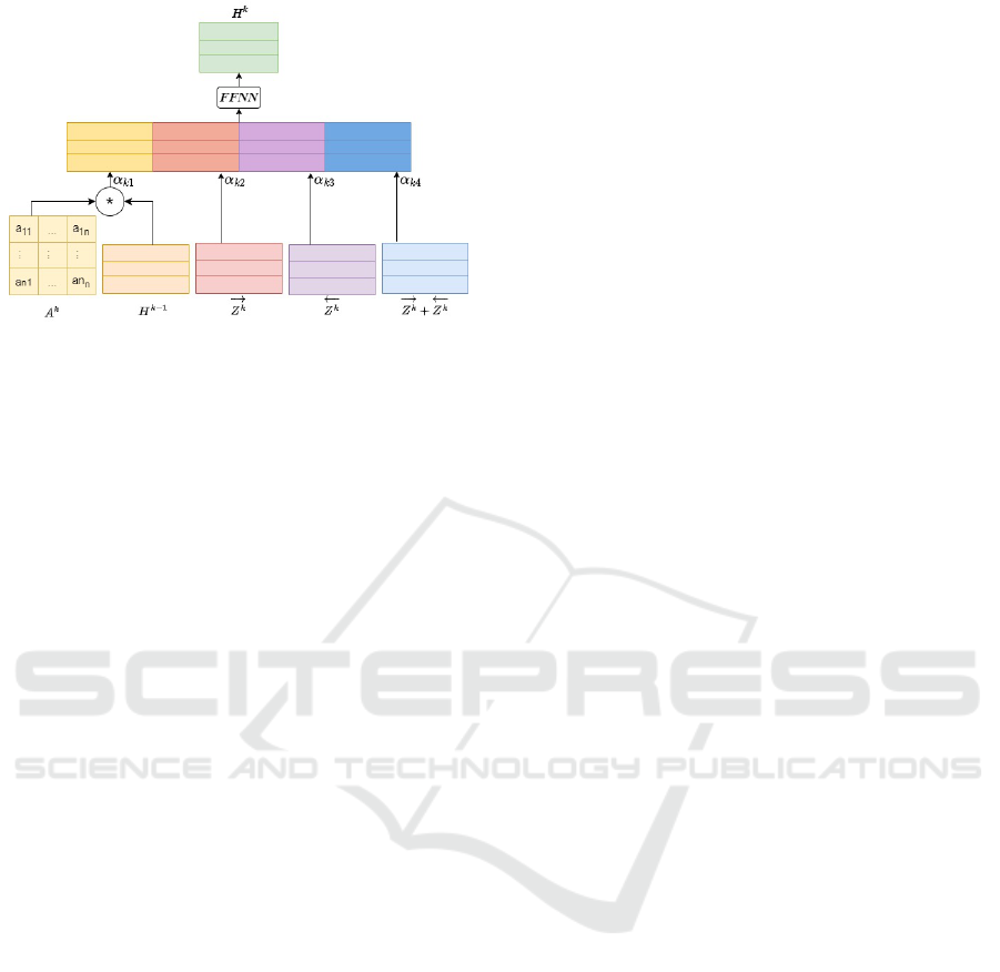
Figure 1: An illustration of k

layer embeddings.

important since it is utilized for graphs, and it is as-

sumed that we can exploit the graph structure deeply.

In some cases, if we are unable to use deeper GCN, its

performance will be marginally higher than the Multi-

Layer Perceptron (MLP). This is due to the presence

of rich initial node features in the majority of the

datasets. As a result, even with just the MLP, we can

achieve some decent results. To overcome the issues

arising from deeper GCNs (Liu et al., 2020), we de-

couple the transformation and propagation.

A recent work (Liu et al., 2020) has used decou-

pled GCN and implements the structure as follows:

Y = so f tmax(A

′

(X)) (5)

where f

(.) is a function that transforms the fea-

tures, for which typically a multilayer perceptron is

used. A

′

is constructed based on graph structure and

propagation strategy. In our work, we adapt the deﬁ-

nition of decoupling as provided by (Liu et al., 2020).

As a result, we use GCN based feature transformation

function, and A

′

is the power adjacency matrix based

on the layer of the model. Our approach decouples

the propagation and transformation operations of typ-

ical GCN by explicitly considering k-hop neighbors

in equation 1 i.e., unlike typical GCN, we multiply

with A

instead of A. This scheme of decoupling prop-

agation and transformation helps create deeper mod-

els without signiﬁcantly affecting performance. This

indicates that the typical drawback of GCN, over-

smoothing, is not observed in a decently deep (40 lay-

ers) GNNDLD model. Though in practice, we usually

do not use a large receptive ﬁeld, however, in the event

of few training nodes, a broad receptive ﬁeld is nec-

essary to include more information. There are some

applications such as social network analysis, where

a large receptive ﬁeld may improve the performance,

but by no means it is sufﬁcient.

The directional label distribution features, along

with the original node features, are helpful in improv-

ing the representation for both graph homophily and

heterophily. The impact of these features is more

prominent in cases of heterophily, as these features

show the distribution of various node labels. In net-

work homophily, the majority of nodes have the same

node type in its surrounding and might have similar

node representation as compared to the heterophilous

network. The embedding of the k

layer for the pro-

posed model is illustrated in Figure 1 and is given as

= FFNN(α

k−1

||α

−→

||α

←−

(

←−

−→

))

(6)

where α ∈ R

kX4

, H

= X, || denotes column-wise

concatenation, and FFNN is feedforward neural net-

work that uses Relu as an activation function.

We take the hidden state vector from all k-layers

and apply max pooling to each node to increase ex-

pressiveness. We next feed the resulting represen-

tation into a feedforward neural network to ﬁnd the

probability distribution of the node labels for classiﬁ-

cation.

Q(Y |G;θ) = FFNN(H

||max(H

, H

..., H

))

(7)

where α and β are learnable parameters and β ∈

. α is learned to decide how much importance is to

be given to node features and label distribution for all

three edge direction channels, whereas β is used to de-

cide how much importance should be given to layer-

wise features. We use cross-entropy loss at the output

layer of our model. Initial node features have been

found to be particularly informative in many graph

datasets. As a result, in addition to taking structurally

updated node features into account through propa-

gation and transformation, we consider initial node

features (H

) that have rich self-knowledge. We are

aware that each layer of a neural network tends to

provide different information, regardless of whether a

graph is heterophilous or homophilous, and thus they

should be addressed accordingly. In typical GCN, the

last hidden state representation is an amalgamation of

information from all k-layers (hops). Sometimes, in

the process of amalgamating information, some im-

portant information gets diluted and some unneces-

sary information gets enhanced. To overcome this

problem we are using the weighted output of each

layer individually. The weighted layer output is fed

into the FFNN to learn which layer features should be

given more importance. This idea is similar to adding

skip connections from every layer with weights (akin

to a ”skip connection” between layers). We employ

an FFNN for our ﬁnal classiﬁcation.

GNNDLD: Graph Neural Network with Directional Label Distribution

169

Intuitions: In equation 6, A

gives the number

of walks of length k between vertices. Studying

these walks provides insights into the graph’s struc-

ture, connectivity, and dynamics. It helps understand

node connectivity and accessibility and is crucial for

measuring node centrality and inﬂuence in the net-

work. If the vertices have a larger number of walks

between them then their features get multiplied by the

number of walks. Unlike GAT (Veli

ckovi

c et al.,

2018), which learns the weight explicitly for each

neighbor our approach implicitly takes weight based

on the number of walks between vertices (utilizing

). Also, A

, captures more structural information

than typical GCN as A

not only shows the connec-

tion/edge between two vertices but also shows how

strongly the two vertices are connected. Traditional

GCNs average node features with those of their neigh-

boring nodes, which is effective in homophily but

may not be effective in heterophily. The nodes in het-

erophily are expected to be connected to various class

nodes, and their representations are distinct from one

another. Therefore, we continue using the initial fea-

tures while also learning new features from various

graph hops. Each layer gathers data differently; the

earliest layers are more local, while the latter ones

gather an increasing amount of global data (implic-

itly, via propagation).

5 EXPERIMENTS

In this section, we examine various GNN models and

assess the performance of the proposed model, GN-

NDLD. Real-world datasets (Luan et al., 2022; Zhu

et al., 2020) are used for node classiﬁcation. We be-

gin by detailing the datasets and experimental setups

used in the model. We compare our model to other

state-of-the-art models and then conduct an ablation

study to validate the model’s various components. Fi-

nally, the performance of GNNDLD is evaluated by

changing the number of layers. We report the average

test accuracy with standard deviation.

5.1 Datasets

We conduct extensive experiments on six datasets

commonly used in the GNN literature for node clas-

siﬁcation tasks. A brief summary of the datasets is

presented in Table 1. In the table, if the homophily

ratio is close to one, the dataset is more homophilic.

On the other hand, if the ratio is close to zero, the

dataset is heterophilic. Homophily is investigated in

citation network datasets such as Cora, CiteSeer, and

PubMed. In these datasets, papers are represented as

nodes, while citations of one publication by another

are represented by edges. The node label of a paper

indicates its academic subject, and the node features

indicate how papers are represented as a bag of words.

For heterophily, three datasets- Chameleon, Squirrel,

Film are considered. Chameleon and Squirrel contain

Wikipedia pages on similar topics. The Film dataset

is a subgraph of the director-actor-writer-ﬁlm graph.

5.2 Experimental Setup and Analysis

Our experiments focus on a transductive environment

in which we have access to all the features of nodes

and a subset of their labels. During training, the

weight of each edge is treated as a free variable.

We compare our model with the following ap-

proaches, 1) Classic GNN models: Vanilla GCN

(Kipf and Welling, 2017), GAT (Veli

ckovi

c et al.,

2018), and GraphSage (Hamilton et al., 2017). 2)

Heterophily focused models: GCNII (Chen et al.,

2020), FSGNN (Maurya et al., 2021), APPNP

(Klicpera et al., 2019), H2GCN (Zhu et al., 2020),

FAGCN (Bo et al., 2021), MixHop (Abu-El-Haija

et al., 2019), and ACM (Luan et al., 2022). 3) Edge

direction focused model: EGNN (Gong and Cheng,

2019) and MagNet (Zhang et al., 2021). 4) Decou-

pled architecture: DAGNN (Liu et al., 2020). We

use the same data splits and training process for all

datasets in order to provide a thorough and fair com-

parison of various models. We use a data split pre-

sented by (Bo et al., 2021), with nodes from each

class accounting for 60%, 20%, and 20% of the to-

tal for training, validation, and testing, respectively.

For our model, the hyperparameter details are given

in Table 2. The searching Hyper-parameters include

learning rate and weight decay for three types of lay-

ers i.e. input layer, hidden layer, and output layer. The

other crucial hyperparameters include epoch, number

of layers, and dropout.

5.2.1 Comparison with Baseline and SOTA

Models

To visualize the performance of our model, we con-

sider real-world datasets with homophily ratios rang-

ing from strong homophily (Cora, CiteSeer, and

PubMed) to strong heterophily (Chameleon, Squirrel,

ﬁlm). Table 3 gives the accuracy and standard de-

viation of GNNDLD and other models. The results

of GCN are from (Zhu et al., 2020), GAT, Graph-

SAGE, GCNII, APPNP, H2GCN, FAGCN, MixHop,

and ACM are from (Luan et al., 2022), FSGNN is

from (Maurya et al., 2021), EGNN is from (Gong

and Cheng, 2019), and MagNet (Zhang et al., 2021).

We have considered the best performance score of ev-

ICAART 2024 - 16th International Conference on Agents and Artiﬁcial Intelligence

170

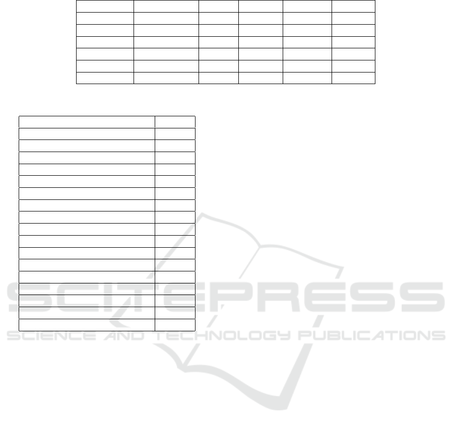
Table 1: Statistics of datasets.

Dataset Hom. Ratio Nodes Edges Features Classes

Cora 0.819 2,708 10,556 1,433 7

CiteSeer 0.703 3,327 9,104 3,703 6

PubMed 0.791 19,717 88,648 500 3

Squirrel 0.22 5,201 198,353 2,089 5

Chameleon 0.23 2,277 36,101 2,325 4

Film 0.22 7,600 33,544 931 5

Table 2: Hyperparameters for GNNDLD.

Hyperparameters Values

weight decay for alpha 0.01

weight decay for beta 0.0001

weight decay for ﬁrst layer 0.001

weight decay for hidden layers 0.0001

weight decay for ﬁnal layer 0.0001

learning rate for alpha 0.01

learning rate for beta 0.01

learning rate for ﬁrst layer 0.01

learning rate for hidden layers 0.01

learning rate for ﬁnal layer 0.01

hidden units 64

epochs 1500

Optimizer Adam

Activation ReLU

dropout 0.6

Layer-wise normalization Yes

Number of layers 3

ery model. We observe that GNNDLD consistently

outperforms across the entire homophily range, from

low to high. The performance improvement of GN-

NDLD over the baseline method GCN is between

5.71% − 45.43%. In two of the heterophily datasets,

Squirrel and Film, GNNDLD outperforms SOTA by

nearly 7.74% and 33.83%, respectively. The perfor-

mance of all existing models on the Film dataset is

consistently poor, i.e., less than 42%, whereas GN-

NDLD could achieve 75.69%. In edge direction fo-

cused models, both EGNN and MagNet perform less

than our model. The accuracy of MagNet greatly de-

grades in the case of homophilous networks. Further-

more, we evaluate DAGNN, a method based on de-

coupling, and ﬁnd that its performance on homophily-

based datasets is inferior compared to GNNDLD

GNNDLD performs better than SOTA on both ho-

mophilous and heterophilous graphs. Overall, the re-

sults indicate that the proposed approach can be gen-

eralized without incurring a high computational cost

for node classiﬁcation tasks in both homophily and

heterophily.

As we cannot include results for all the current

state-of-the-art methods, we referred to Papers With

Code (https://paperswithcode.com/), a free platform

for researchers and professionals to explore the latest

advancements in machine learning research papers,

code implementations, and datasets. The results were

directly obtained from Papers With Code, and our

analysis reveals that our proposed approach outper-

forms all the other methods across various datasets.

Comprehensive results of SOTA approaches are pro-

vided in Appendix A.

5.2.2 Ablation Study

In this section, we consider the effects of various com-

ponents of the proposed model. Table 4 shows the

comparison of the proposed model with other vari-

ants of the model. The ﬁrst variant, GNNDLD-1,

only considers the initial features of nodes and does

not consider directional label distribution. The second

variant, GNNDLD-2 uses the initial features of nodes

with label distribution without considering edge di-

rection. The third variant, GNNDLD-3, considers the

initial features of nodes with directional label distri-

bution without decoupling. As per our observations

from Table 4, the label distribution adds a lot of in-

formation to node features. The directional label dis-

tribution has more impact on a heterophilous dataset

than on a homophilous one.

GCN suffers from oversmoothing in the case of

heterophily graphs such as chameleon, squirrel, and

ﬁlm. GNNDLD-1, which models decoupling, is able

to give better results in the case of heterophily when

compared to GCN. In the case of homophily, over-

smoothing works in favor of node label classiﬁcation,

which is visible from the GCN results. In GNNDLD-

2, the addition of label distribution improves both ho-

mophily and heterophily graphs signiﬁcantly. The

proposed model, GNNDLD, adds direction informa-

tion to the GNNDLD-2 variant, and it is evident that

there is a slight improvement in homophily graphs

and a signiﬁcant improvement in heterophily graphs.

In GNNDLD-3, we remove the decoupling mecha-

nism and observe that it performs poorly in cases of

heterophily graphs due to oversmoothing. This indi-

cates that the directional label distribution is resilient

to oversmoothing.

GNNDLD: Graph Neural Network with Directional Label Distribution

171

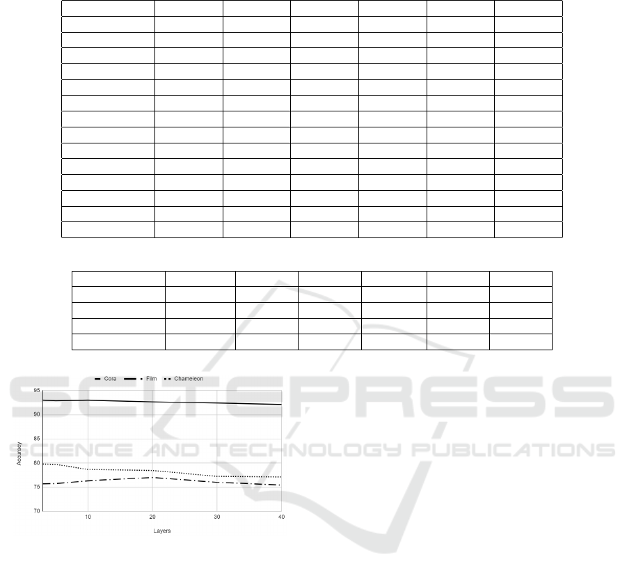
Table 3: Comparison of GNNDLD with baseline and SOTA models: mean test accuracy (%) and standard deviation. The best

results are highlighted in bold format and ”N/A” indicates results not reported in the paper.

Datasets / Models Cora CiteSeer PubMed Chameleon Squirrel Film

GCN 87.28±1.26 76.68±1.64 87.38±0.66 59.82±2.58 36.89±1.34 30.26±0.79

GAT 76.70 ± 0.42 67.20 ± 0.46 83.28 ± 0.12 63.9 ± 0.46 42.72 ± 0.33 35.98 ± 0.23

GraphSAGE 86.58 ± 0.26 78.24 ± 0.30 86.85 ± 0.11 62.15 ± 0.42 41.26 ± 0.26 36.37 ± 0.21

GCNII 88.93 ± 1.37 81.83 ± 1.78 89.98 ± 0.52 62.8 ± 2.87 38.31 ± 1.3 41.54 ± 0.99

FSGNN 87.73±1.36 77.19±1.35 89.73±0.39 78.14±1.25 73.48±2.13 35.67±0.69

APPNP 79.41 ± 0.38 68.59 ± 0.30 85.02 ± 0.09 51.91 ± 0.56 34.77 ± 0.34 38.86 ± 0.24

H2GCN 87.52 ± 0.61 79.97 ± 0.69 87.78 ± 0.28 52.30 ± 0.48 30.39 ± 1.22 38.85 ± 1.17

FAGCN 88.85 ± 1.36 82.37 ± 1.46 89.98 ± 0.54 49.47 ± 2.84 42.24 ± 1.2 31.59 ± 1.37

MixHop 87.61±0.85 76.26±1.33 85.31±0.61 60.50±2.53 43.80±1.48 32.22±2.34

EGNN (best) 88.8 ± 0.3 77.1 ± 0.4 86.7 ± 0.1 N/A N/A N/A

MagNet 79.8±2.5 67.5±1.8 N/A N/A N/A N/A

DAGNN 84.4 ± 0.5 73.3 ± 0.6 80.5 ± 0.5 N/A N/A N/A

ACM (best) 89.75 ± 1.16 82.28 ± 1.12 91.44 ± 0.59 76.08 ± 2.13 69.98 ± 1.53 41.86 ± 1.48

GNNDLD 92.99 ±0.9 86.3±1.24 91.95±0.19 79.78±1.66 77.72±0.84 75.69±0.78

Table 4: Ablation study on different components in GNNDLD. The best results are highlighted in bold format.

Datasets / Models Cora CiteSeer PubMed Chameleon Squirrel Film

GNNDLD-1 84.044 ±1.35 73.6±1.59 88.35±0.43 69.67±2.17 56.66±8.24 32.89±0.67

GNNDLD-2 92.89±1.03 85.68±1.02 92.88±0.29 71.58±2.52 57.75±1.8 73.14±0.85

GNNDLD-3 92.13±1.06 85.38±1.06 91.88±0.28 78.53±1.94 76.29± 1.0 73.71±0.63

GNNDLD 92.99 ±0.9 86.3±1.24 91.95±0.19 79.78±1.66 77.72±0.84 75.69±0.78

Figure 2: Analysis of GNNDLD with an increase in the

number of layers (k) for two types of datasets, 1) Ho-

mophily - Cora 2) Heterophily- Film and Chameleon.

5.2.3 Oversmoothing

To explore the occurrence of oversmoothing, we run

an experiment with varying layers (k) in the model.

GNNDLD is compared for both heterophilous and

homophilous datasets as shown in Figure 2. For

heterophily, we use the Chameleon and Film datasets.

In the case of heterophily, we observe that GNNDLD

has a slightly lower performance from k=3 to k=10,

after which the performance is nearly constant. In

the case of the Film dataset, the performance peaks

at k=20. In the case of homophily, we consider

Cora and the performance is almost constant for

all k values. This analysis shows that the over-

smoothing issue that traditional GCN has is being

addressed by GNNDLD. Due to oversmoothing,

the performance of GCN (Liu et al., 2020) in the

heterophily and homophily based datasets starts to

decline when k is greater than 8 (Rusch et al., 2023).

6 CONCLUSION

We focused on utilizing intrinsic graph information

such as direction and label distribution around a node.

Such information is understudied, and we highlighted

that these simple concepts can boost the performance

of GNN greatly. We demonstrate how our model can

adapt to both homophily and heterophily graphs by

taking into account features from all of the model’s

layers with directional label distribution. Empirically,

this approach shows strong performance across both

heterophily and homophily datasets. In the future,

we would like to add some attention mechanisms that

might further improve the node representation in het-

erophily.

ACKNOWLEDGEMENTS

We are thankful to Indo-Japanese (DST-JST) Joint

Lab Grant on Intelligent CPS for supporting this

ICAART 2024 - 16th International Conference on Agents and Artiﬁcial Intelligence

172

project. This work has also been supported by Na-

tional Security Council Secretariat (NSCS), Govt. of

India.

REFERENCES

Abu-El-Haija, S., Perozzi, B., Kapoor, A., Alipourfard, N.,

Lerman, K., Harutyunyan, H., Steeg, G. V., and Gal-

styan, A. (2019). MixHop: Higher-order graph con-

volutional architectures via sparsiﬁed neighborhood

mixing. In Chaudhuri, K. and Salakhutdinov, R., edi-

tors, Proceedings of the 36th International Conference

on Machine Learning, volume 97 of Proceedings of

Machine Learning Research, pages 21–29. PMLR.

Bo, D., Wang, X., Shi, C., and Shen, H. (2021). Be-

yond low-frequency information in graph convolu-

tional networks. In AAAI, pages 3950–3957.

Chen, M., Wei, Z., Huang, Z., Ding, B., and Li, Y. (2020).

Simple and deep graph convolutional networks. In

III, H. D. and Singh, A., editors, Proceedings of the

37th International Conference on Machine Learning,

volume 119 of Proceedings of Machine Learning Re-

search, pages 1725–1735. PMLR.

Defferrard, M., Bresson, X., and Vandergheynst, P. (2016).

Convolutional neural networks on graphs with fast

localized spectral ﬁltering. In Proceedings of the

30th International Conference on Neural Information

Processing Systems, NIPS’16, page 3844–3852, Red

Hook, NY, USA. Curran Associates Inc.

Dong, H., Chen, J., Feng, F., He, X., Bi, S., Ding, Z., and

Cui, P. (2021). On the equivalence of decoupled graph

convolution network and label propagation. In Pro-

ceedings of the Web Conference 2021, WWW ’21,

page 3651–3662, New York, NY, USA. Association

for Computing Machinery.

Fu, X., Zhang, J., Meng, Z., and King, I. (2020). Magnn:

Metapath aggregated graph neural network for hetero-

geneous graph embedding. In Proceedings of The Web

Conference 2020, WWW ’20, page 2331–2341, New

York, NY, USA. Association for Computing Machin-

ery.

Geisler, S., Li, Y., Mankowitz, D., Cemgil, A. T.,

unnemann, S., and Paduraru, C. (2023). Transform-

ers meet directed graphs.

Gong, L. and Cheng, Q. (2019). Exploiting edge features

for graph neural networks. In 2019 IEEE/CVF Con-

ference on Computer Vision and Pattern Recognition

(CVPR), pages 9203–9211.

Grover, A. and Leskovec, J. (2016). Node2vec: Scal-

able feature learning for networks. In Proceedings

of the 22nd ACM SIGKDD International Conference

on Knowledge Discovery and Data Mining, KDD ’16,

page 855–864, New York, NY, USA. Association for

Computing Machinery.

Guo, Y. and Wei, Z. (2023). Graph neural networks with

learnable and optimal polynomial bases.

Hamilton, W. L., Ying, R., and Leskovec, J. (2017). Induc-

tive representation learning on large graphs. In Pro-

ceedings of the 31st International Conference on Neu-

ral Information Processing Systems, NIPS’17, page

1025–1035, Red Hook, NY, USA. Curran Associates

Inc.

He, K., Zhang, X., Ren, S., and Sun, J. (2016). Deep resid-

ual learning for image recognition. In 2016 IEEE Con-

ference on Computer Vision and Pattern Recognition

(CVPR), pages 770–778.

He, Y., Gan, Q., Wipf, D., Reinert, G. D., Yan, J., and Cu-

curingu, M. (2022). GNNRank: Learning global rank-

ings from pairwise comparisons via directed graph

neural networks. In Chaudhuri, K., Jegelka, S., Song,

L., Szepesvari, C., Niu, G., and Sabato, S., editors,

Proceedings of the 39th International Conference on

Machine Learning, volume 162 of Proceedings of Ma-

chine Learning Research, pages 8581–8612. PMLR.

Hu, Y., You, H., Wang, Z., Wang, Z., Zhou, E., and Gao,

Y. (2021). Graph-mlp: Node classiﬁcation without

message passing in graph.

Kipf, T. N. and Welling, M. (2017). Semi-supervised clas-

siﬁcation with graph convolutional networks.

Klicpera, J., Bojchevski, A., and G

unnemann, S. (2019).

Predict then propagate: Graph neural networks meet

personalized pagerank. In 7th International Confer-

ence on Learning Representations, ICLR 2019, New

Orleans, LA, USA, May 6-9, 2019. OpenReview.net.

Li, G., Muller, M., Thabet, A., and Ghanem, B. (2019).

Deepgcns: Can gcns go as deep as cnns? In 2019

IEEE/CVF International Conference on Computer Vi-

sion (ICCV), pages 9266–9275, Los Alamitos, CA,

USA. IEEE Computer Society.

Li, Q., Han, Z., and Wu, X.-M. (2018). Deeper in-

sights into graph convolutional networks for semi-

supervised learning. In Proceedings of the Thirty-

Second AAAI Conference on Artiﬁcial Intelligence

and Thirtieth Innovative Applications of Artiﬁcial In-

telligence Conference and Eighth AAAI Symposium

on Educational Advances in Artiﬁcial Intelligence,

AAAI’18/IAAI’18/EAAI’18. AAAI Press.

Lim, D., Hohne, F., Li, X., Huang, S. L., Gupta, V.,

Bhalerao, O., and Lim, S.-N. (2021). Large scale

learning on non-homophilous graphs: New bench-

marks and strong simple methods.

Liu, M., Gao, H., and Ji, S. (2020). Towards deeper graph

neural networks. In Proceedings of the 26th ACM

SIGKDD International Conference on Knowledge

Discovery& Data Mining, KDD ’20, page 338–348,

New York, NY, USA. Association for Computing Ma-

chinery.

Luan, S., Hua, C., Lu, Q., Zhu, J., Zhao, M., Zhang, S.,

Chang, X., and Precup, D. (2021). Is heterophily A

real nightmare for graph neural networks to do node

classiﬁcation? CoRR, abs/2109.05641.

Luan, S., Hua, C., Lu, Q., Zhu, J., Zhao, M., Zhang, S.,

Chang, X.-W., and Precup, D. (2022). Revisiting het-

erophily for graph neural networks.

Ma, J., Cui, P., Kuang, K., Wang, X., and Zhu, W.

(2019). Disentangled graph convolutional networks.

In Chaudhuri, K. and Salakhutdinov, R., editors, Pro-

ceedings of the 36th International Conference on Ma-

GNNDLD: Graph Neural Network with Directional Label Distribution

173

chine Learning, volume 97 of Proceedings of Machine

Learning Research, pages 4212–4221. PMLR.

Maurya, S. K., Liu, X., and Murata, T. (2021). Improv-

ing graph neural networks with simple architecture de-

sign.

Pei, H., Wei, B., Chang, K. C.-C., Lei, Y., and Yang, B.

(2020). Geom-gcn: Geometric graph convolutional

networks.

Peng, H., Zhang, R., Dou, Y., Yang, R., Zhang, J., and

Yu, P. S. (2021). Reinforced neighborhood selection

guided multi-relational graph neural networks. ACM

Trans. Inf. Syst., 40(4).

Poiitis, M., Sermpezis, P., and Vakali, A. (2022). Pointspec-

trum: Equivariance meets laplacian ﬁltering for graph

representation learning. In 2022 IEEE/WIC/ACM In-

ternational Joint Conference on Web Intelligence and

Intelligent Agent Technology (WI-IAT), pages 315–

320.

Rong, Y., Huang, W., Xu, T., and Huang, J. (2020). Drope-

dge: Towards deep graph convolutional networks on

node classiﬁcation.

Rusch, T. K., Bronstein, M. M., and Mishra, S. (2023). A

survey on oversmoothing in graph neural networks.

Scarselli, F., Gori, M., Tsoi, A. C., Hagenbuchner, M.,

and Monfardini, G. (2009). The graph neural net-

work model. IEEE Transactions on Neural Networks,

20(1):61–80.

Veli

ckovi

c, P., Cucurull, G., Casanova, A., Romero, A., Li

P., and Bengio, Y. (2018). Graph attention networks.

Wang, H. and Leskovec, J. (2020). Unifying graph convo-

lutional neural networks and label propagation.

Wang, H. and Leskovec, J. (2021). Combining graph convo-

lutional neural networks and label propagation. ACM

Trans. Inf. Syst., 40(4).

Xu, K., Li, C., Tian, Y., Sonobe, T., Kawarabayashi, K.-

i., and Jegelka, S. (2018). Representation learning on

graphs with jumping knowledge networks. In Dy, J.

and Krause, A., editors, Proceedings of the 35th Inter-

national Conference on Machine Learning, volume 80

of Proceedings of Machine Learning Research, pages

5453–5462. PMLR.

Yan, Y., Hashemi, M., Swersky, K., Yang, Y., and Koutra,

D. (2022). Two sides of the same coin: Heterophily

and oversmoothing in graph convolutional neural net-

works. In 2022 IEEE International Conference on

Data Mining (ICDM), pages 1287–1292, Los Alami-

tos, CA, USA. IEEE Computer Society.

Yao, G., Lei, T., and Zhong, J. (2019). A review

of convolutional-neural-network-based action recog-

nition. Pattern Recognition Letters, 118:14–22. Co-

operative and Social Robots: Understanding Human

Activities and Intentions.

Zhang, X., He, Y., Brugnone, N., Perlmutter, M., and Hirn,

M. (2021). Magnet: A neural network for directed

graphs. In Ranzato, M., Beygelzimer, A., Dauphin,

Y., Liang, P., and Vaughan, J. W., editors, Advances in

Neural Information Processing Systems, volume 34,

pages 27003–27015. Curran Associates, Inc.

Zhao, L. and Akoglu, L. (2019). Pairnorm: Tackling over-

smoothing in gnns. CoRR, abs/1909.12223.

Zhong, Z., Ivanov, S., and Pang, J. (2022). Simplifying

node classiﬁcation on heterophilous graphs with com-

patible label propagation.

Zhu, J., Rossi, R. A., Rao, A., Mai, T., Lipka, N., Ahmed,

N. K., and Koutra, D. (2021). Graph neural networks

with heterophily.

Zhu, J., Yan, Y., Zhao, L., Heimann, M., Akoglu, L., and

Koutra, D. (2020). Beyond homophily in graph neural

networks: Current limitations and effective designs.

APPENDIX

To conduct a detailed performance comparison

between GNNDLD and existing approaches, we

refer the Papers With Code website and extracted the

state-of-the-art (SOTA) results for all six datasets.

The following graphs are directly sourced from the

website, and the metric used for comparison in all the

graphs is mean test accuracy. Table 5 presents the

best existing approach till date for all the datasets with

their mean test accuracy values. Figure 3 to Figure 8

shows the mean test accuracy graphs for dataset Cora,

CiteSeer, PubMed, Chameleon, Squirrel, and Film,

respectively. In all the graphs x-axis represents the

SOTA approach sorted based on their publishing year

and y-axis represents their mean test accuracy (%).

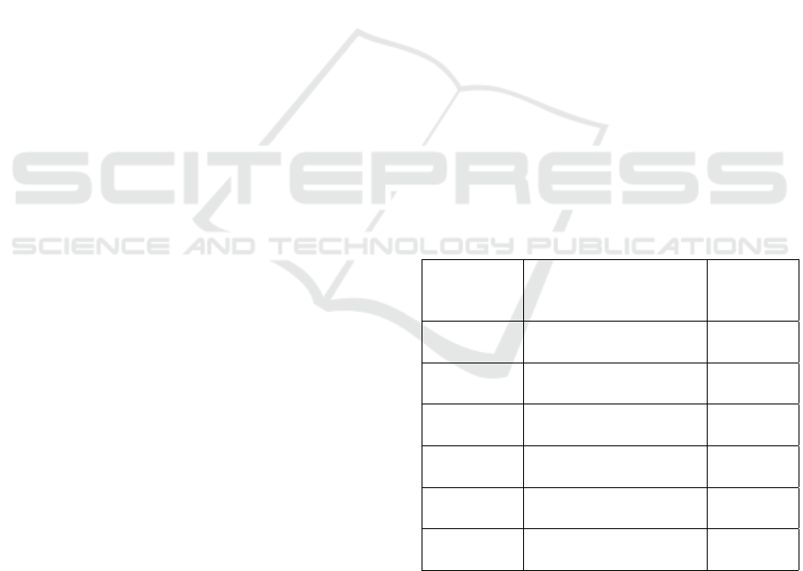
Table 5: Datasets with their best performing approach and

their respective mean test accuracy values.

Dataset SOTA Approach Mean test

accuracy

(%)

Cora ACM-GCN+ (Bo

et al., 2021)

91.17

CiteSeer FAGCN (Bo et al.,

2021)

83.48

PubMed ACM-Snowball-3

(Luan et al., 2022)

91.91

Chameleon ACM-GCN+ (Luan

et al., 2022)

78.21

Sqirrel ACMII-GCN++

(Luan et al., 2022)

71.51

Film FavardGNN (Guo and

Wei, 2023)

43.05

ICAART 2024 - 16th International Conference on Agents and Artiﬁcial Intelligence

174

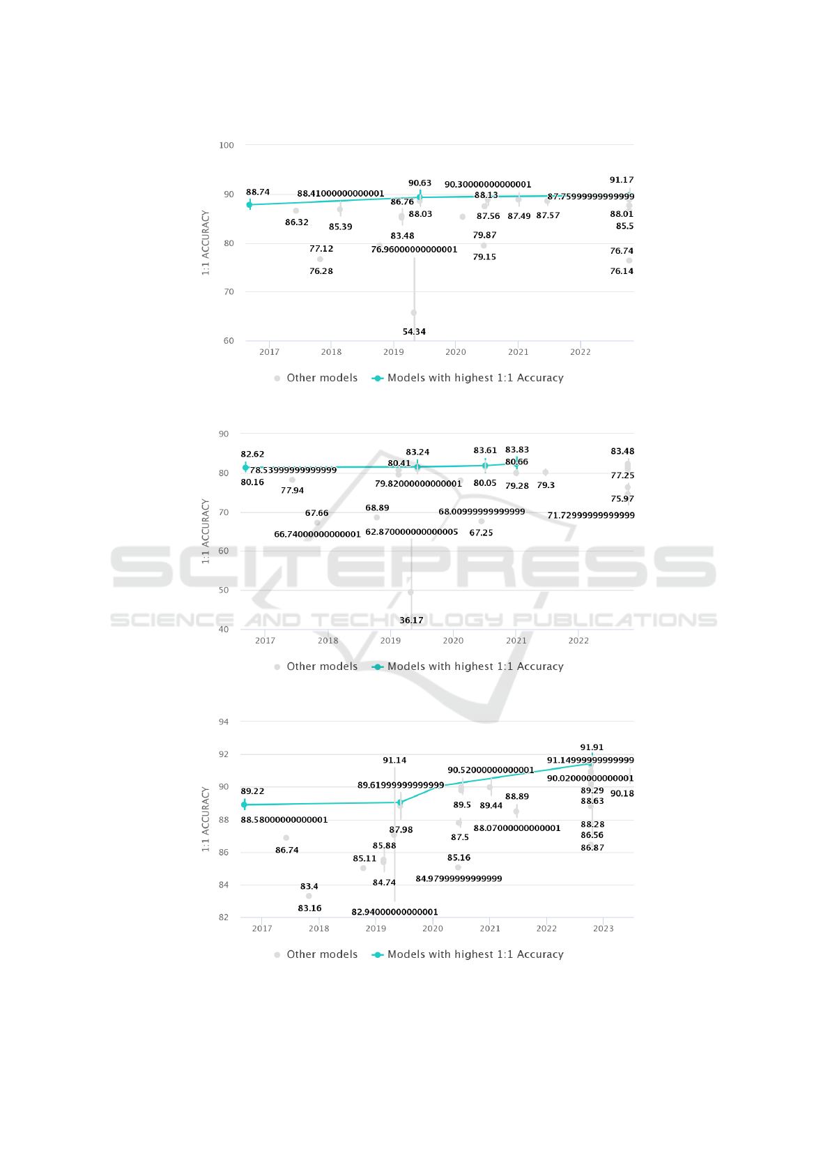
Figure 3: Comparative Performance of Node Classiﬁcation Methods on the Cora Dataset.

Figure 4: Comparative Performance of Node Classiﬁcation Methods on the CiteSeer Dataset.

Figure 5: Comparative Performance of Node Classiﬁcation Methods on the PubMed Dataset.

GNNDLD: Graph Neural Network with Directional Label Distribution

175

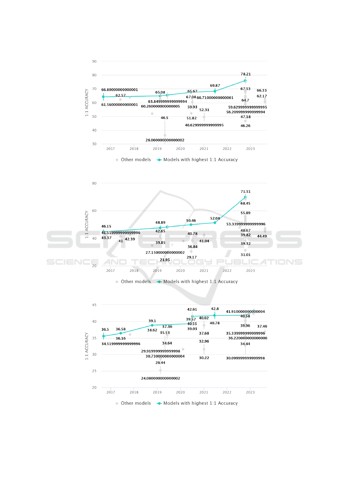
Figure 6: Comparative Performance of Node Classiﬁcation Methods on the Chameleon Dataset.

Figure 7: Comparative Performance of Node Classiﬁcation Methods on the Squirrel Dataset.

Figure 8: Comparative Performance of Node Classiﬁcation Methods on the Film Dataset.

ICAART 2024 - 16th International Conference on Agents and Artiﬁcial Intelligence

176