HierNet: Image Recognition with Hierarchical Convolutional Networks
Levente Tempfli
1 a
and Csan
´
ad S
´
andor
2 b
1
School of Computation, Information and Technology, Technical University of Munich, Germany
2
Faculty of Mathematics and Computer Science, Babes¸–Bolyai University, Cluj-Napoca, Romania
fl
Keywords:
Convolutional Neural Networks, Image Classification, Category Hierarchy.
Abstract:
Convolutional Neural Networks (CNNs) have proven to be an effective method for image recognition due to
their ability to extract features and learn the internal representation of the input data. However, traditional
CNNs disregard the hierarchy of the input data, which can lead to suboptimal performance. In this paper,
we propose a novel method of organizing a CNN into a quasi-decision tree, where the edges represent the
feature-extracting layers of a CNN and the nodes represent the classifiers. The structure of the decision tree
corresponds to the hierarchical relationships between the label classes, meaning that the visually similar classes
are located in the same subtree. We also introduce a simple semi-supervised method to determine these
hierarchical relations to avoid having to manually construct such a hierarchy between a large number of classes.
We evaluate our method on the CIFAR-100 dataset using ResNet as our base CNN model. Our results show
that the proposed method outperforms this base CNN between 2.12-3.77% (depending on the version of the
architecture), demonstrating the effectiveness of incorporating input hierarchy into CNNs. Code is available
at https://github.com/levtempfli/HierNet.
1 INTRODUCTION
In the area of Deep Learning, the problem of im-
age classification is one of the most fundamental and
heavily researched problems. The introduction of
Convolutional Neural Networks (CNNs) was a ma-
jor breakthrough in the field (LeCun et al., 1998;
Krizhevsky et al., 2012). Since then, the appearance
of more sophisticated architectures and training algo-
rithms built on CNNs has increased the performance
of models year by year (Krizhevsky et al., 2012; Si-
monyan and Zisserman, 2015; He et al., 2016; Tan
and Le, 2019).
Traditional CNNs are built sequentially with layer
after layer starting with an input layer and ending with
some flattening and fully connected layer(s). The idea
behind these networks is that the convolutional oper-
ation acts on a small area of the input, thus detecting
small details. Convolutions can extract lower-level
features in the earlier layers, while higher-level fea-
tures in the last layers. This way, a stack of convolu-
tional layers can learn the general visual representa-
tion of an object accurately. However, these sequen-
tial models disregard the hierarchy of the data classes
a
https://orcid.org/0009-0008-5930-0901
b
https://orcid.org/0000-0001-6666-0114
and treat every class equally distinguishable. In real-
ity, groups of classes have similar visual appearances
(e.g., a dog is similar to a cat, while a tulip is much
more similar to other flowers than to animals).
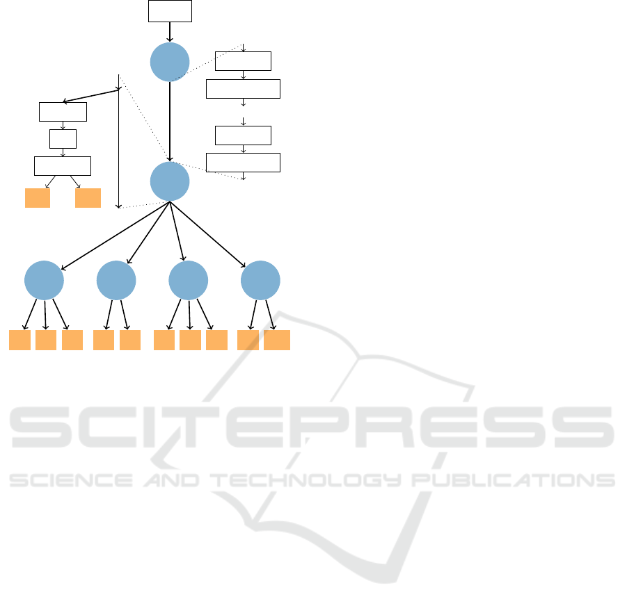
In this paper, we introduce HierNet, a CNN ar-
chitecture that exploits the hierarchy between the
classes. HierNet is organized in a tree-like architec-
ture and can be conceptualized as a decision tree (see
Figure 1). The difference is that the edges in our
tree represent convolutional, feature-extracting oper-
ations, and in the nodes happens the classification of
which route should be taken next (based on the ex-
tracted features in the preceding edge). The categories
outputted by the leaf nodes represent the predicted
class. Although we have to train the whole tree, dur-
ing inference we only have to evaluate just one route
from the root node to a leaf node based on the outputs
of the classifications in the nodes.
To construct our model, we need the hierarchy
of the classes represented as a tree. In such a tree,
the classes are the leaves, and the internal nodes are
the super-classes (or groups of classes) of its child
nodes. While a small number of categories can be
constructed manually, we introduce a method for cre-
ating such a hierarchical tree in an automated way to
handle classification problems with hundreds of cate-
Tempfli, L. and Sándor, C.
HierNet: Image Recognition with Hierarchical Convolutional Networks.
DOI: 10.5220/0012321100003636
Paper published under CC license (CC BY-NC-ND 4.0)
In Proceedings of the 16th International Conference on Agents and Artificial Intelligence (ICAART 2024) - Volume 2, pages 147-155
ISBN: 978-989-758-680-4; ISSN: 2184-433X
Proceedings Copyright © 2024 by SCITEPRESS – Science and Technology Publications, Lda.
147

image
v
1
v
2
e
1
v
3
e
2
c
1
c
2
c
3
v
4
e
3
c
4
c
5
v
5
e
4
c
6
c
7
c
8
v
6
e
5
c
9
c
10
Flatten
FC
Softmax
c
v
3
...
c
v
6
Conv2D
BatchNorm
...
Conv2D
BatchNorm
Figure 1: Basic architecture of HierNet. The edges con-
tain the operations the same as the backbone. In the nodes,
the output of the previous edge is connected to subsequent
edges and to the classification module that outputs the next
node.
gories.
Introducing the hierarchy of classes and internal
nodes also improves the explainability of the net-
work’s decision: compared to a traditional convolu-
tional neural network (where one can only get the out-
put probabilities), HierNet also outputs the probabili-
ties produced by the internal nodes. This information
helps to understand why a certain prediction is made,
and in case of an incorrect decision, it also facilitates
architectural improvement by indicating which part of
the architecture needs to be extended to improve ac-
curacy.
We summarize our main contributions as follows:
• We introduce HierNet, a tree-like CNN architec-
ture that exploits the hierarchy between classes.
• We present a semi-supervised method to cluster
classes into super-classes based on their hierarchi-
cal relations.
• We analyze and compare the results of HierNet
and its backbone model using the CIFAR-100
dataset.
2 RELATED WORK
One of the first papers that introduced a hierarchical
deep CNN architecture for image classification is HD-
CNN (Yan et al., 2015). This work uses a coarse cate-
gory CNN classifier to separate easy classes, and fine
category classifiers for more challenging classes. The
method is built upon a building block CNN, which
can be chosen from top-ranked single CNNs. HD-
CNN probabilistically integrates predictions from fine
category classifiers and achieves lower error with a
manageable increase in memory and classification
time. The main disadvantages of this method are
the slow training time (due to the separate training of
coarse and fine classifiers) and the lack of possibility
to scale to hierarchical classification tasks that have
more than two levels.
A similar approach to ours is the Adaptive Neural
Trees (ANT) (Tanno et al., 2019). ANT has a tree-
shaped architecture with convolutional layers on the
edges (so-called ”transformers”) and classifiers in the
nodes (so-called ”routers” in the internal nodes and
”solvers” in the leaf nodes.). During inference, only
one route is selected. Compared to our method, the
main difference is that their leaf nodes output all of
the classes, and the hierarchy of the tree is not based
on the logical hierarchy between classes: their hierar-
chy is built dynamically during training by randomly
adding leaf nodes and edges, keeping them if they im-
prove the model accuracy, and discarding the change
if they don’t.
Attention Convolutional Binary Trees (ACNet) is
another tree-shaped architecture with convolutional
operations along the edges and routers in the nodes (Ji
et al., 2020). ACNet is constrained to use a binary tree
structure with a pre-defined depth, the operations on
the edges are asymmetrical, and the results are from
the accumulation of leaves.
(Zhu and Bain, 2017) introduces Branch Convo-
lutional Neural Network or B-CNN. This work also
uses a predefined hierarchical tree of classes. Al-
though it has a sequential model, there are classifiers
at various depths of the CNN to predict super-classes
and, finally, the classes in the last classifier. Consider-
ing the classifiers of the super-classes are earlier than
those of the child classes, this paper showed that the
feature extractions learned to classify a super-class
could be reused for subsequent classifiers.
3 MODEL DESCRIPTION
The task of HierNet is learning to classify image
samples into c categories, formally to learn the con-
ICAART 2024 - 16th International Conference on Agents and Artificial Intelligence
148

ditional distribution p(y|x) from a {x
(i)
,y
(i)
}
i∈[[1,N]]
dataset, where x
(i)
∈ X denotes an image, y
(i)
∈ Y
the corresponding label, and N the number of train-
ing samples; X and Y is the set of training images and
the set of c labels, respectively. Next, we present the
basic architecture of HierNet, how the training is per-
formed, and three techniques to enhance the model’s
accuracy.
3.1 Basic Architecture
The architecture is organized around a decision tree,
so we define the architecture with a H = (T,F,C)
triad, where T denotes the topology of the tree, F the
feature extracting operations performed on the edges
and C the classifier operations conducted in the nodes.
Topology. Considering it is a tree, the T topology of
the tree consists of a V set of nodes and E set of edges,
where V = {v
1
,v
2
,...v
n
} and E = {e
1
,e
2
,...,e
m
} =
{(a,b) : a, b ∈ V,a ̸= b}, where (a, b) means that b
is the child of a. There is one and only one root
node root ∈ V without a parent (|{(a,b) : b = root,a ∈
V } ∩ E| = 0) and every other v ∈ V \{root} node has
only one parent (|{(a,b) : b = v,a ∈ V }∩E| = 1). This
topology is constructed from the hierarchy between
the c classes obtained either manually based on the
logical hierarchy or with an algorithm based on a con-
fusion probability matrix (as described in Section ‘4).
Operations. Every edge is assigned with zero or
more feature-extracting operations f ∈ F.
We denote with f
i, j
the j-th operation of the e
i
edge, where i ∈ {1,m}, j ∈ {1,k
i
} and k
i
is the num-
ber of operations in the i-th edge. The direction of
the operations is from the parent node to the child
node. The edge e
i
can be considered as the function
f
i,k
◦ f
i,k−1
◦ ··· ◦ f
i,2
◦ f
i,1
, where f
i,1
gets the input
from the preceding edge (except from f
1,1
, where the
input is the model input – the image). f
i,k
operation’s
output is fed into the next edges (if there are any) as
well as to the classifier of the v
i+1
node. Technically,
a feature extracting operation could be any continu-
ous, derivable function with arbitrary input and out-
put dimensions, but considering that our task is im-
age classification, we use the usual operations used in
convolutional neural networks, like convolutional lay-
ers, batch normalization (Ioffe and Szegedy, 2015),
max pooling and ReLU. It is important to note that
an operation’s output dimension must match the next
operation’s input dimension requirements.
Classification. Every node v
i
(where i > 1) contains
a classifier function c
i
The role of these nodes is the
same as the nodes of a decision tree: to decide to-
wards which child node to send the samples from
the current node route (to which sub-tree). The c
i
function is the composition of 3 functions/operations,
c
i
(x) = c
i,3
(c
i,2
(c
i,1
(x))), where the input of c
i,1
is the
output of the incoming edge. The role of c
i,1
is to
flatten its input by applying a simple flattening or a
Global Average Pooling. The c
i,2
is a fully connected
layer with v
i
out
output neurons, where v
i
out
is the num-
ber of child edges (or child nodes) of v
i
. Formally:
c
i,2
(x) = W ·x + b with W weights and b biases. c
i,3
is
a Softmax function, that outputs a probability distri-
bution over the v
i
out
options. This is used for deciding
the next route by selecting the one with the highest
probability. Let c
e
j
i
be the probability predicted for the
direction towards edge e
j
(or v
k
), where e
j
parent
= v
i
and e
j
child
= v
k
.
The root node of the tree is an exception since
there is no need to classify the input image without
feature extraction. So the root node simply forwards
the input image to f
1,1
.
Backbone Model. For the operations on the edges,
we use the same operations in the same order that
are present in standard CNNs, like ResNet (He et al.,
2016) or VGG16 (Simonyan and Zisserman, 2015).
We call these the ”backbone” models of HierNet. Ev-
ery operation (or layer) present in the backbone model
is spread out from the edge after the root node to the
edges before the leaves. Since the output of an edge is
connected to the inputs of every subsequent edge, op-
erations from the root node to a leaf node are the same
as the operations from the input to the output of the
backbone model. The classifications in the nodes are
an exception because the backbone model only has a
classification function at the end of the model. In con-
trast, HierNet has classifiers at every node (except the
root node), and the number of possible output classes
at a leaf node is much smaller. It is configurable how
we would like to split up the operations of the back-
bone model among the edges on a root-to-leaf path,
but we made a constraint that every edge at an i level
must have the same operations. Figure 2 illustrates the
relation between our model and a backbone model.
During Prediction. We carry out the classification
of the input image the following way: apply all the
operations on the edge after the route node; feed the
output of the operations to the classification function
in the first node after the root; choose a sub-branch
based on the output of the classification function; ap-
ply all the operations in the sub-branch on the feature
HierNet: Image Recognition with Hierarchical Convolutional Networks
149

HierNet Backbone
v
1
v
1
f
1,1
f
1
f
1,2
f
2
f
1,3
f
3
v
2
v
2
v
3
v
4
v
5
f
2,1
f
2,2
f
2,3
v
3
f
3,1
f
3,2
f
3,3
v
4
f
4,1
f
4,2
f
4,3
v
5
f
4
f
5
f
6
v
3
Figure 2: Relation between the HierNet and a backbone
network. The different colors represent the different oper-
ations/layers. The operations follow the same architecture
and order as in the backbone model. The edges on the same
level have the same set of operations.
map obtained previously; feed the output of the last
operations to the first node on the sub-branch; con-
tinue the cycle until reaching a leaf; the classifier in
the leaf should give back the correct class of the in-
putted image in that node. An outputted class in a
leaf node can be transformed easily into a global class
number because we know the order of leaf nodes.
Considering only the operations from the root to a
leaf are evaluated, and the operations on a root-to-
leaf route are exactly the same as the backbone model,
the evaluation time during prediction should be simi-
lar to the backbone model with the slight addition of
the classifiers in the nodes. The pseudocode of the
algorithm used during prediction is presented in Al-
gorithm 1.
Input: input - an RGB image
e ← e[1];
x ← e(x) // e(x) = f
k
(... f
2
( f
1
(x))...)
v ← v[2] // v(x) = c(x), where c = c
i
class ← v(x);
while v /∈ V
lea f s
do
e ← v
child edges
[class];
v ← v
child nodes
[class];
x = e(x);
class = v(x);
end
class ← global class prediction form class
and v;
Algorithm 1: HierNet prediction algorithm.
3.2 Training
HieNet can be trained end-to-end, like the baseline
model. To achieve this, each of the outputted prob-
abilities of the leaf nodes is multiplied by all the
outputted probabilities of the ancestor nodes leading
to that leaf. Formally, let R
v
i
be the set of edges
on the route from the root to v
i
and o
i
is the new
outputted probability distribution of v
i
. In this case
o
i
= c
i
∗
∏
j∈R,k∈{k:v
k
=e
j
parent
}
c
e
j
k
. Then the new clas-
sification outputs of the leaf nodes are concatenated
from left to right. Because only one route corresponds
to an outputted class, there are altogether c number of
categories outputted by the leaf nodes, and we got our
output.
It’s important to note that the order of the out-
putted classes depends on the hierarchical tree given.
Hence, it is necessary for every model to reorder the
labels in the dataset; the categories of the true label’s
one-hot representation match the intended place of
that label in the hierarchy.
We can report two accuracies for every model: a
”conditional accuracy” and a ”routing accuracy.” The
former is calculated from the predictions by the out-
put during training (the concatenated o
j
-s), while the
latter is by following the route from the root to a
leaf based on the classifier outputs of the nodes (the
method outlined in section 3.1 or Algorithm 1).
We use Categorical Cross-entropy loss for the
training of HierNet As far as the training algorithm,
learning rate, or other similar hyperparameters are
concerned, we usually use the same configuration as
the baseline model.
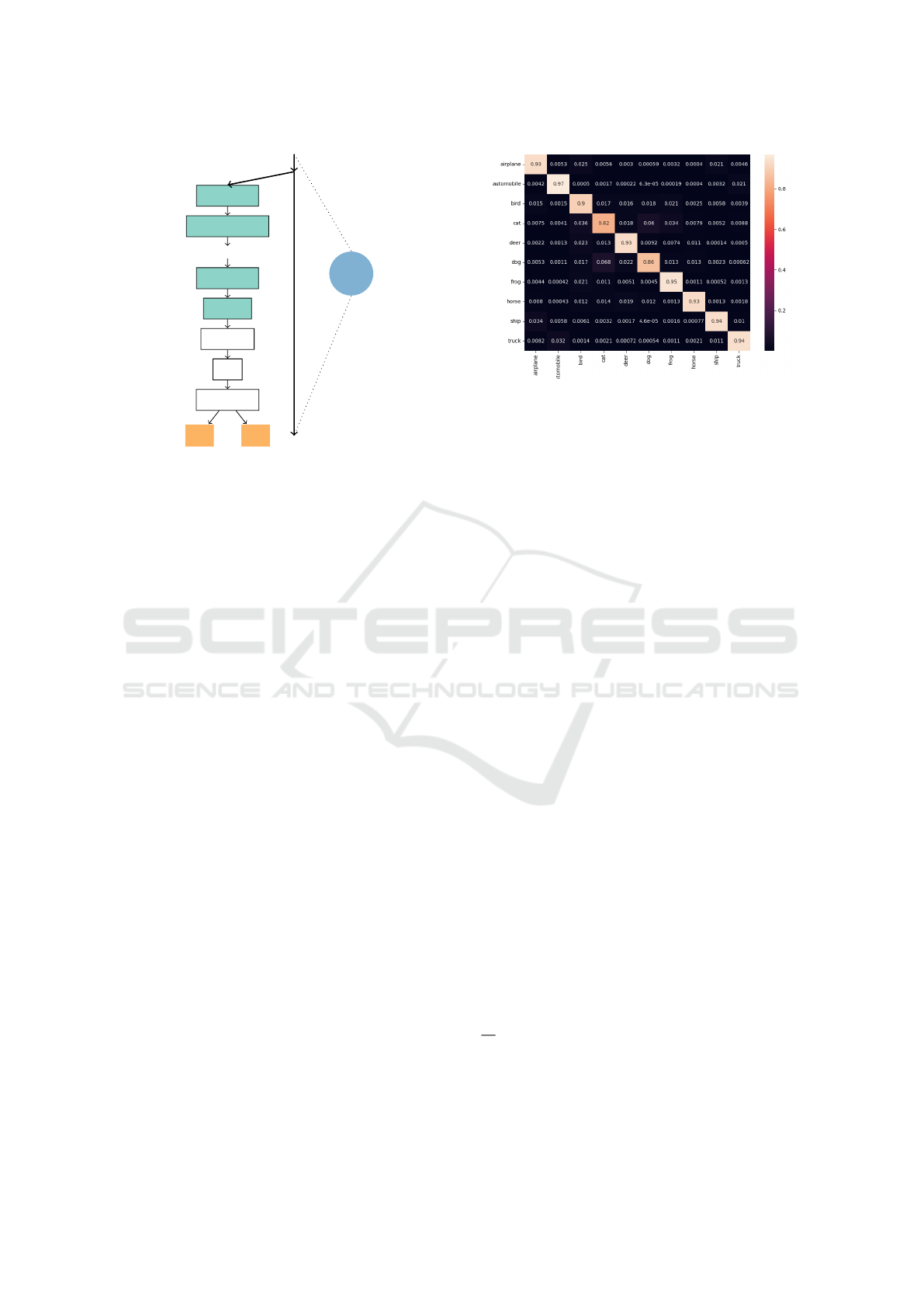
3.3 Additional Layers Before the
Classifier
We present a modification of the architecture in the
nodes to increase their accuracy: Adding a few addi-
tional layers between the input from the edge and the
flattening by the classification function. An illustra-
tion of this modification is shown in Figure 3.
The motivation behind this is that categorizing
into super-classes might require different, indepen-
dent features extracted. Previously the feature map
used by the classifier in the nodes was the same as
the feature map passed to the subsequent layer. But
with this modification, there are additional operations
on that feature map that are only used for the classifi-
cations. These extra layers might extract the features
specific for super-classes categorized by that node.
The additional layers added after the edge input
also follow the backbone model’s architecture. Con-
sidering the last operation from the previous edge cor-
ICAART 2024 - 16th International Conference on Agents and Artificial Intelligence
150

v
2
Conv2D
BatchNorm
...
Conv2D
ReLU
Flatten
FC
Softmax
c
v
3
...
c
v
6
Figure 3: Slight modification of the node: Additional fea-
ture extracting layers (with green background) before the
classifiers to increase node accuracy.
responds to a layer from the backbone model, the few
k added layers in the node correspond to the following
k layers in the backbone model.
The leaf nodes are an exception because we can-
not assign any additional layers to them. The reason
behind this is that the architecture of a root-to-leaf
path is the same as the backbone architecture; hence
the input of the leaf nodes is the output of the last
layer of the backbone model therefore, there are no
remaining layers after the last one to add to the nodes.
The drawback of this approach is the slightly in-
creased model size. Previously during prediction, the
evaluation complexity of a route from the root to a leaf
was similar to the evaluation complexity of the back-
bone model, just with a small surplus of the evalua-
tion of the classifier functions in the nodes. With this
approach, this difference increases by the evaluation
complexity of the added operations in every touched
node, so it is crucial not to overshoot the number of
added layers.
4 HIERARCHY CONSTRUCTION
The topology of our model is constructed from a tree
that represents the hierarchy between the c classes of
the dataset. The leaves of this tree are the c classes,
and the internal nodes represent the super-classes. In
an ideal hierarchical tree, if the visual difference is
small for two classes, the probability of being in the
same super-class is high.
While a hierarchy can be constructed manually for
a few dozen classes, this could be time-consuming
Figure 4: The confusion probability matrix of the 10
CIFAR-10 classes from the validation set evaluated on the
ResNet backbone (n = 5).
when there are hundreds or thousands of classes.
Moreover, a hierarchy constructed by humans may
not be the best option for CNNs: one could say that a
bird and an airplane should belong to the same super-
class since both of them have wings but for the net-
work, their visual similarity is not close at all. To
tackle this problem, we construct the hierarchy based
on the confusion probability matrix of the network.
Confusion Probability Matrix. To group the cat-
egories, we need to have some information about
the visual similarity relations between the classes.
For this, we create a confusion probability matrix
(CPM) similar to a confusion matrix. In a CPM’s
row (corresponding to a true label) the predicted
probabilities are accumulated instead of the predicted
classes. Then every row is divided by the number
of examples belonging to that true label, so the row
contains the average probabilities that represent the
chance of a true class being predicted as another class.
CPM[i][ j] = p represents the probability of an image
with i class being predicted as j class. We construct
the CPM with the trained backbone evaluated on the
validation set. An example with the CPM matrix is
shown in Figure 4.
Grouping Algorithm. To group c number
of classes into g groups based on the CPM,
we define the proximity of classes c
1
, c
2
as
dist(c
1
,c
2
) = CPM[c
1
][c
2
] + CPM[c
2
][c
1
] – the
back and forth confusion probabilities). The prox-
imity of two groups is defined by dist(G
1
,G
2
) =
1
|T |
∑
(c
1
,c
2
)∈T
(CPM[c
1
][c
2
] + CPM[c
2
][c
1
]), where
T = G
1
× G
2
= {(c
1
,c
2
) : c
1
∈ G
1
,c
2
∈ G
2
} – the
average of proximities of all combinations of classes
from the two groups.
The grouping works by first considering every
HierNet: Image Recognition with Hierarchical Convolutional Networks
151

class a different group. It merges the two groups with
the highest proximity at every iteration until there are
no more possible group pairs to merge. During group-
ing, the following constraints are considered: (1) The
combined sizes of the two groups cannot exceed the
g
max
predefined value; (2) The proximity of the two
groups has to exceed the p
min
value. The second one
is necessary to only group classes together that are
close enough and the first one is to avoid too large
groups when the others are small by cardinality.
Although this algorithm only creates groups of
classes from a set of classes, thus resulting in a hi-
erarchical tree with a depth of 2 (level 0: root; level
1: nodes representing the groups, level 2: nodes rep-
resenting the classes), applying it recursively on the
created groups will result in sub-groups, thus deeper
trees.
5 EXPERIMENTS
In this section, we will discuss the results of our
method. First, we will discuss the hyperparameters
that define our model, the range of these parameters
that we tested, and what we found to be the recom-
mended values. Then we will discuss the metrics and
datasets used, followed by the reference models used,
software/hardware configurations, and finally the re-
sults and comparisons.
5.1 Hyperparemeters
Besides the backbone (or reference) model used and
the traditional hyperparameters (e.g. learning rate,
batch size, number of epochs), each HierNet is de-
fined by 4 specific parameters.
Split Point of Backbone CNN. Since the convolu-
tional and other feature-extracting layers are in the
same order on a route from root to leaf as in a se-
quential backbone network, we need to define a split
point. Such a point defines how many of the first lay-
ers belong to the common edge before the first classi-
fier, while the rest belong to the edges leading to the
leaf nodes. We tested with split points ranging from
30% to 85% of the total number of layers. According
to the experiments, lower split points (30 − 50%) per-
formed worse, while higher ones yielded higher accu-
racy, meaning that our model seems to require more
feature extraction for the superclass decision than for
the fine class decision. Although high split points
generally performed better, too high of a split point
(85 − 90%) also resulted in a decrease in accuracy,
meaning that the optimal range is around 70 − 75%.
Number of Additional Classifier Layers. We pre-
sented in 3.3 a modification that increases the accu-
racy of our model by adding some independent lay-
ers for the superclass classifier node. We empiri-
cally showed that the more layers added, the better
the performance, which is understandable because the
model has more parameters to learn the representa-
tion, but it also increases the evaluation time. Adding
just 4% − 12% of the total number of layers as addi-
tional independent layers had a significant increase in
performance compared to not adding any layers at all.
While adding 16%−25% gave even better results, the
leap was not as big as going from 0% to 4% − 12%.
Minimum Proximity of Group Members. The
structure of our tree is defined by the hierarchy or
groups created by our grouping algorithm. One of
the parameters that define the groups produced is the
minimum required proximity of the members of a
group (as described in 4). We have found this to be
the much more important parameter because it gener-
ally defines the allowed variety of objects in a group,
and hence the number of groups. Having too few or
too many groups resulted in a significant drop in per-
formance, and in our case of 100 classes, the opti-
mal number of groups we found was around 6 − 8.
The minimum proximity parameter should be set to
achieve a similar number of groups, in our case it was
around 0.005 − 0.0075.
Maximum Size of Each Group. Restricting the
size of a group turned out to be a much less useful pa-
rameter than minimum proximity. We compared sev-
eral cases where the number of groups was the same,
but in one case it was produced by high p
min
and low
g
max
, and in the other by low p
min
and high g
max
. We
found that controlling the size of a group with p
min
was much more beneficial, so we later decided to just
set g
max
to 50. This allowed quite large groups but still
didn’t allow more than half of the classes to belong to
just one group, which would defeat the purpose.
5.2 Metrics
For our task of classification, we use accuracy as the
metric to measure performance, just like the authors
of (He et al., 2016; Shah et al., 2016). A HierNet
model can be evaluated in two ways, so naturally we
can calculate two different accuracies for each model.
The fast evaluation method is to evaluate only one
branch or path of the decision tree based on the deci-
sion in the superclass classifier node, thus making the
prediction in only one leaf node. The much slower but
ICAART 2024 - 16th International Conference on Agents and Artificial Intelligence
152

slightly more accurate evaluation method is to evalu-
ate every branch of the decision tree for an input im-
age and, similar to training, we can construct a prob-
ability vector by multiplying the output probabilities
along the path to a leaf node, thus predicting from
all classes. Having two evaluation methods means
having two reportable accuracies. The fast scoring
method can be used in cases where higher accuracy
is desired with similar performance as the backbone
network. Conversely, the slower scoring method can
be used when performance is less important.
5.3 Dataset
We use the CIFAR-100 (Krizhevsky et al., 2009)
dataset for our experiments. It consists of 60000 RGB
images with a resolution of 32 × 32 containing 100
classes, each class containing 600 images.
This dataset is more suitable for our purposes
than the CIFAR-10 dataset by the same authors
(Krizhevsky et al., 2009), because it has significantly
more classes that are less feasible to group manually,
allowing us to test the effectiveness of our grouping
algorithm. On the other hand, it has much fewer im-
ages of much lower resolution than ImageNet (Rus-
sakovsky et al., 2015), allowing us to train it on our
own hardware.
Originally, the dataset is split into two sets, one
containing 50000 images, and the other 10000. We
use the first set for training, but we further split the
second set into a validation set and a test set, both
containing 5000 images with the same number of im-
ages per class. We use the validation set to evaluate
the backbone model, to construct the groupings from
the confusion probability matrix, and then to perform
hyperparameter tuning. In this way, we avoid leak-
ing information from the test set into the training, and
we may evaluate the test set only once. The reported
accuracies are measured on the test set.
We use the same 2 image augmentations as the au-
thors of (He et al., 2016), namely: random horizontal
flip and random translation with a factor of 0.125 on
both the horizontal and vertical axis, where the pixels
outside the image are filled with grey.
5.4 ResNet: the Backbone Model
We use two types of ResNet (He et al., 2016) architec-
tures as our backbone reference models: the original
ResNet (He et al., 2016) and a ResNet that uses ELUs
(Shah et al., 2016) (Exponential Linear Units (Clevert
et al., 2015)).
Architecture. Like the authors of (Shah et al.,
2016), we do not use the regular ResNet architec-
ture tailored for ImageNet, but the smaller version
used by the original authors of ResNet (He et al.,
2016) for classifying CIFAR-10 images. The origi-
nal authors(He et al., 2016) define network sizes of
n = {3,5, 7, 9, 18}, where they first have a convo-
lutional layer, followed by 3 × n stacks of residual
blocks, where each stack of residual blocks has half
the feature map size and twice the number of filters of
the previous stack, starting from 32x32 and 16. In the
case of the ResNet with ELU activations (Shah et al.,
2016), they are also based on this architecture, the dif-
ference is in the structure of the residual blocks. In
both cases, we use the same architecture, i.e. a route
from the root node to a leaf node corresponds exactly
to a ResNet (or ELU ResNet), with the slight differ-
ence of the additional superclass classifier branch and
the reduced fully connected layer (and softmax out-
put) sizes in the leaves. We define the number of ad-
ditional classifier layers and split points in terms of
the number of residual blocks rather than individual
layers (but to get the number of layers, multiply by 2
and add 2).
Training. In terms of training, we trained with al-
most the same hyperparameters as the original authors
(He et al., 2016). Namely, we use gradient descent
with a batch size of 128, a weight decay of 0.0001,
and a momentum of 0.9, but there is a slight differ-
ence in the learning rate schedule. All HierNets use a
similar schedule to the n = 18 ResNet, namely, we use
0.01 to warm up the network for 2000 iterations, then
we use 0.1 to 32K, 0.01 to 48K, and 0.001 after that.
We have found that transfer learning (transferring the
weights of a trained backbone CNN to a HierNet) is
very beneficial, so we perform it before each training
of a HierNet. We re-implemented the backbone mod-
els, trained them, and used the resulting accuracies as
a reference.
5.5 Software and Hardware
Configurations
For ease of implementation, all HierNet and back-
bone ResNet models were implemented in Python
3.8.10 using TensorFlow v2.7.0. The tf.Data input
pipeline was used to load the dataset and a custom
non-sequential keras. The model was defined to con-
tain the HierNet architecture. We ran the tests on
a machine equipped with 16GB of RAM, an Intel
7600K CPU, and an Nvidia GTX 1080TI GPU. The
training time was about 1.5-2 hours for the smaller
ResNet models of size 20 and 4-5 hours for ResNets
HierNet: Image Recognition with Hierarchical Convolutional Networks
153

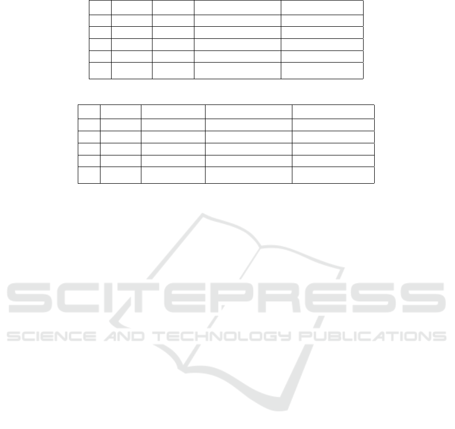
Table 1: Comparison of the accuracy of our HierNet and the backbone ResNet for different network sizes.
n #layers ResNet Ours w/ slow eval. Ours w/ fast eval.
3 20 65.96 68.89 68.08
5 32 67.08 70.65 70.45
7 44 68.12 71.25 70.75
9 56 68.38 72.15 72.01
18 110 71.33 73.45 73.27
Table 2: Comparison of the accuracy of our HierNet and the backbone ELU ResNet for different network sizes.
n #layers ELU ResNet Ours w/ slow eval. Ours w/ fast eval.
3 20 65.54 68.30 68.16
5 32 67.88 70.71 70.43
7 44 68.79 70.83 70.79
9 56 69.03 72.47 72.29
18 110 72.93 74.37 74.15
with 110 layers.
5.6 Grouper Algorithm Results
We would like to briefly present the results of our
grouping algorithm to show that the groups produced
do indeed contain visually similar classes. The fol-
lowing groupings have been generated based on the
confusion probability matrix of the backbone ResNet
(n = 9) with the settings p
min
= 0.0075 and g
max
= 50:
• GROUP 1: baby, girl, woman, boy, man
• GROUP 2: palm tree, forest, pine tree, willow
tree, maple tree, oak tree
• GROUP 3: aquarium fish, trout, flatfish, ray,
shark, dolphin, whale
• GROUP 4: wardrobe, chair, television, bed,
couch, keyboard ...
• ...
5.7 HierNet Results
Finally, we present the performance of our HierNet
model in comparison to the ResNets (He et al., 2016;
Shah et al., 2016). The accuracies are reported for
the test set, which was evaluated only once after the
hyperparameter tuning had been completed.
Table 1 shows the performance improvements
provided by our HierNet architecture compared to us-
ing a regular, sequential ResNet. As well as improv-
ing for each network size, the accuracy of the small-
est HierNet (n = 3) is comparable to that of the second
largest ResNet (n = 9), and the second largest HierNet
outperforms the largest ResNet (n = 18) by 0.82%,
despite being half the length. In terms of parame-
ters, each run had the grouping parameters g
m
ax = 50
and p
m
in = 0.0075, additional classifier blocks of
{2,3,4,5,4} and split points of {5,9,12,16,38}. The
latter two were defined in residual blocks, not layers.
Table 2 shows the results with the ResNet using
ELU activations. As in the previous case, our Hi-
erNet has better performance for each network size,
and smaller HierNets come close to or even exceed
the performance of much larger ResNets. In every
case, g
m
ax was set to 50 and p
m
in was set to 0.005,
additional classifier blocks to {2, 3, 2, 5, 4} and split
points to {6,9,15,19,38}.
We can see a slight difference between our two
evaluation methods, with the slower one tending to
have a slightly higher accuracy. This is understand-
able because by training the whole tree, not just a
branch, we are training the network on the output of
the slow evaluation method, so the increase in accu-
racy of the faster method is just a ’by-product’ of the
training.
6 CONCLUSION
This paper presented HierNet, a convolutional neural
network architecture. HierNet exploits the visual sim-
ilarities and hierarchy between classes. We achieved
this by constructing a tree for the hierarchical rela-
tionships, where the edges represent the feature ex-
traction convolutions and the nodes have the classifier
or routing function. In this way, classes in the same
group can share the feature extraction operation, but
be independent of the other groups.
The results of our experiments confirm that this
ICAART 2024 - 16th International Conference on Agents and Artificial Intelligence
154

architecture works as intended. And although we
outperformed the backbone networks in almost every
case, there is room for improvement.
An improvement might be a more sophisticated
grouping algorithm. Our grouping algorithm often
produces group trees where, for example, one group
has 40 classes while others have only a few. Although
it’s probably impossible to construct a completely bal-
anced tree, because some classes are more distinct
while another large set of classes are more similar,
we could improve our algorithm to take into account
how balanced the hierarchy tree is.
Regarding training, since we used the same opti-
mizer, learning rate schedule, and weight decay as for
the backbone models, it is very likely that what works
for the baseline models is not optimal for HierNet, so
we could also investigate the training settings more.
Finally, it might be useful to investigate which
features are extracted by the shared edges and which
features are extracted by the edges of the individual
groups. We could visualize this with an approach sim-
ilar to the one described in (Zeiler and Fergus, 2014).
REFERENCES
Clevert, D.-A., Unterthiner, T., and Hochreiter, S.
(2015). Fast and accurate deep network learning
by exponential linear units (elus). arXiv preprint
arXiv:1511.07289.
He, K., Zhang, X., Ren, S., and Sun, J. (2016). Deep
Residual Learning for Image Recognition. In Pro-
ceedings of 2016 IEEE Conference on Computer Vi-
sion and Pattern Recognition, CVPR ’16, pages 770–
778. IEEE.
Ioffe, S. and Szegedy, C. (2015). Batch normalization: Ac-
celerating deep network training by reducing internal
covariate shift. In International conference on ma-
chine learning, pages 448–456. PMLR.
Ji, R., Wen, L., Zhang, L., Du, D., Wu, Y., Zhao, C., Liu,
X., and Huang, F. (2020). Attention convolutional bi-
nary neural tree for fine-grained visual categorization.
In Proceedings of the IEEE/CVF Conference on Com-
puter Vision and Pattern Recognition, pages 10468–
10477.
Krizhevsky, A., Hinton, G., et al. (2009). Learning multiple
layers of features from tiny images.
Krizhevsky, A., Sutskever, I., and Hinton, G. E. (2012).
Imagenet classification with deep convolutional neu-
ral networks. In Pereira, F., Burges, C. J. C., Bottou,
L., and Weinberger, K. Q., editors, Advances in Neu-
ral Information Processing Systems 25, pages 1097–
1105. Curran Associates, Inc.
LeCun, Y., Bottou, L., Bengio, Y., and Haffner, P. (1998).
Gradient-based learning applied to document recogni-
tion. In Proceedings of the IEEE, volume 86, pages
2278–2324.
Russakovsky, O., Deng, J., Su, H., Krause, J., Satheesh,
S., Ma, S., Huang, Z., Karpathy, A., Khosla, A.,
Bernstein, M., Berg, A. C., and Fei-Fei, L. (2015).
ImageNet Large Scale Visual Recognition Challenge.
International Journal of Computer Vision (IJCV),
115(3):211–252.
Shah, A., Kadam, E., Shah, H., Shinde, S., and Shingade,
S. (2016). Deep residual networks with exponential
linear unit. In Proceedings of the third international
symposium on computer vision and the internet, pages
59–65.
Simonyan, K. and Zisserman, A. (2015). Very deep con-
volutional networks for large-scale image recognition.
In Bengio, Y. and LeCun, Y., editors, 3rd Interna-
tional Conference on Learning Representations, ICLR
2015, San Diego, CA, USA, May 7-9, 2015, Confer-
ence Track Proceedings.
Tan, M. and Le, Q. (2019). EfficientNet: Rethinking model
scaling for convolutional neural networks. In Chaud-
huri, K. and Salakhutdinov, R., editors, Proceedings of
the 36th International Conference on Machine Learn-
ing, volume 97 of Proceedings of Machine Learning
Research, pages 6105–6114. PMLR.
Tanno, R., Arulkumaran, K., Alexander, D., Criminisi, A.,
and Nori, A. (2019). Adaptive neural trees. In In-
ternational Conference on Machine Learning, pages
6166–6175. PMLR.
Yan, Z., Zhang, H., Piramuthu, R., Jagadeesh, V., DeCoste,
D., Di, W., and Yu, Y. (2015). Hd-cnn: Hierarchical
deep convolutional neural networks for large scale vi-
sual recognition. In 2015 IEEE International Confer-
ence on Computer Vision (ICCV), pages 2740–2748.
Zeiler, M. D. and Fergus, R. (2014). Visualizing and under-
standing convolutional networks. In European confer-
ence on computer vision, pages 818–833. Springer.
Zhu, X. and Bain, M. (2017). B-cnn: branch convolutional
neural network for hierarchical classification. arXiv
preprint arXiv:1709.09890.
HierNet: Image Recognition with Hierarchical Convolutional Networks
155