Detection of Energy Drifts in Waste Water Treatment Plants Using

Dynamic Clustering

Lucie Martin

, Muriel Dugachard

, Yuqi Wang

and Guillaume Scherpereel

Veolia Research and Innovation, Chemin de la Digue, Maisons-Lafﬁtte, France

Keywords:

Dynamic Clustering, K-Means, PLS Regression, Energy Consumption, Drift Detection,

Waste Water Treatment Plants.

Abstract:

The sanitation process is energy intensive. There are therefore environmental issues for treated wastewater

companies which must always optimize and reduce their energy expenditure. This paper aims to characterize

the energy consumption patterns of the Waste Water Treatment Plants (WWTPs). Once these patterns have

been established, their evolution is monitored through time. This work is based on the 78 most energy-intensive

treated wastewater treatment plants in France. The consumption is studied from 2019 to the beginning of

2020. Energy expenditure depends on the operating condition of the WWTP, such as the volume of treated

wastewater, the organic-based pollution, the rainfall, the amount of suspended solids, the temperature and

the pH of the efﬂuent. This relation is modeled using PLS regression, which can be used to characterize the

WWTP’s energy consumption behavior. WWTPs’ load patterns are grouped into clusters using K-means.

Five different consumption patterns are obtained for the year 2019. A dynamic K-means is employed to

update patterns on a daily basis. Potentials drifts may have been detected thanks to the statistical distances of

the treatment plants compared to the average characteristics of each of the groups.

1 INTRODUCTION

Sewage treatment and more specially Waste Water

Treatment Plants (WWTPs) are energy-consuming.

Aerator blowers and the pumps are the most signif-

icant consumers of energy in a wastewater treatment

system. Water pumps are used for water transporta-

tion whereas aeration’s systems are used during the

biological treatment. Oxygen is diffused in the water

and consumed by bacteria. The organic-based pollu-

tion, nitrogen and phosphorus are removed by those

bacteria.

To reach a lower CO

footprint and to reduce

costs, wastewater treatment companies are invited to

reduce and manage their energy efﬁciency. Those

objectives are described in the (ISO 50001, 2018)

standard. This standard implies better energy con-

sumption measurement, more efﬁcient use, reduced

consumption and continuous improvement of energy

management.

https://orcid.org/0009-0002-6864-1181

https://orcid.org/0009-0001-1894-6692

https://orcid.org/0000-0003-1022-9135

https://orcid.org/0009-0005-4534-336X

Better energy consumption monitoring is reﬂected

in deployment of sensors in WWTPs and the use of

Machine Learning algorithm. For instance, (Harrou

et al., 2021) uses Machine Learning to detect en-

ergy consumption drifts. Furthermore, (Bagherzadeh

et al., 2021) tries different feature selection methods

to explain and predict energy consumption of the Mel-

bourne East WWTP.

To improve energy management, a recurrent idea

is to compare those forecasts with real data. This is

an intra-plant analysis and does not compare with en-

ergy consumption of other WWTPs. However, it can

be done by grouping together WWTPs following their

energy consumption behavior (i.e. load pattern recog-

nition). Thus, it is possible to identify WWTPs with

lower energy costs and better behavior. Once types

of patterns are deﬁned, it can be interesting to ana-

lyze how they evolved. A change in energy consump-

tion pattern through time can be an energetic drift or

the effect of a corrective action. The proposed solu-

tion for energy management improvement is to use

dynamic clustering methods on WWTPs energy con-

sumption.

Most of the research on energy consumption clus-

tering focus on households and buildings expendi-

Martin, L., Dugachard, M., Wang, Y. and Scherpereel, G.

Detection of Energy Drifts in Waste Water Treatment Plants Using Dynamic Clustering.

DOI: 10.5220/0012320500003654

Paper published under CC license (CC BY-NC-ND 4.0)

In Proceedings of the 13th International Conference on Pattern Recognition Applications and Methods (ICPRAM 2024), pages 661-670

ISBN: 978-989-758-684-2; ISSN: 2184-4313

661

tures. There are few works on industrial plants and

even more speciﬁcally WWTPs. Clustering methods

on WWTPs energy consumption are used to charac-

terize the daily plant inputs. In (Borzooei et al., 2020),

K-Means and Gaussian Mixtures are computed on

meteorological data to identify weather characteris-

tics. Those characteristics are used in a physical

model of energy consumption estimation. (Qiao and

Zhou, 2018) clustered daily efﬂuent concentrations

with Density-Peak method to train Neural Network

on different water quality characteristics. (Li et al.,

2019) is using the same principle replacing Density-

Peak clustering by Fuzzy C-Means and Neural Net-

work by RBF and Linear Regression.

Thus there is a lack in the domain. No cluster-

ing between WWTPs energy consumption seems to

have been done. What tells the state of the art on load

pattern recognition in general? (Rajabi et al., 2020)

gives a comparative study of time series clustering

techniques applied on energy consumption. Most of

them are using K-Centroid methods such as K-Means

or Fuzzy C-Means. The study also explores Hierar-

chical clustering, Probabilistic methods and Density-

Peak clustering.

Energy consumption are times series. Thus, raw

data and summarized ones can both be used. Summa-

rized data can imply a loss of information. However,

raw data can be very time consuming even more if

used with speciﬁc distances, such as Dynamic Time

Warping (Sard

a-Espinosa, 2018). (Shahzadeh et al.,

2015) compared the use of Full Load Pattern, Aver-

age Daily Load Pattern and Regression Coefﬁcients

as inputs of the K-Means. The best results are found

for Regression Coefﬁcients. (Wang et al., 2016) de-

composed the loads in different state with the SAX

methods. Then, Markov Chains allow to model the

consumption behavior. Adaptive K-Means are run on

the Markov chains transition matrices. In this case

study, the number of WWTP and the amount of miss-

ing data impose to summarized data. The aim of the

paper is to deﬁne WWTP energy consumption behav-

ior by summarizing data.

A lot of papers focus on dynamic versions of clus-

tering. General articles such as (M

arquez et al., 2018)

or (Silva et al., 2014) present dynamic clustering for

data streams. However, a few papers explore this

subject in energy load pattern recognition. Among

them, (Ben

ıtez et al., 2016) studied dynamic cluster-

ing of daily loads for households consumption. Eu-

clidean and Hausdorff distances were both analysed

to obtains energy consumption trajectories. But, this

method uses hourly consumptions that are not avail-

able here. Thus what kind of dynamic clustering al-

gorithm can be implemented to ﬁt this data?

Table 1: Number of WWTPs represented per biological pro-

cess.

Biological Process Number of WWTPs

Activated Sludge 51

Bioﬁlter 18

Membrane BioReactor 4

Moving Bed Bioﬁlm Reactor 4

Sequencing Batch Reactor 1

Other 1

This paper proposes a method to dynamically

cluster WWTPs by their energy consumption pat-

terns. It tries to answer the following questions: How

to deﬁne WWTP energy consumption pattern? And,

how to monitor clusters evolution?

Section 2 details the case study and the proposed

method. Section 3 describes all the results obtained.

Finally, Section 4 explains the choices made and

presents the future works.

2 CASE STUDY AND METHODS

2.1 Case Study

This study focuses on 78 municipal WWTPs from the

200 most energy consuming plants operated by Veo-

lia in France. For each WWTP, the biological process

is known. Number of plants per process are presented

in Table 1. Usually, processes with a small footprint

such as Sequencing Batch Reactors (SBR), Mem-

brane Bioreactors (MBR) or Moving Bed Bioﬁlm Re-

actor (MBBR) are supposed to be more energy con-

suming (Stricker et al., 2017).

Besides the process, the plants size in population

equivalent (PE) is given. It can be deﬁned as the num-

ber of people the plant has been designed for. In this

study, the smallest plant size is 50 000 PE.

The activity inside the plant can be represented

by two indicators: treated wastewater volume and

level of contamination. This level is measured by the

Chemical Oxygen Demand (COD). It is a measure of

organic-based pollution. Volume of treated wastew-

ater (m³) is a daily measure whereas the COD (kg)

measures frequency depends of the plant size. That

introduces missing data.

For each plant, the daily energy gross consump-

tion in kWh is known. Often, the gross energy con-

sumption is highly correlated with the size of the

plant. The biggest WWTPs usually consume more

than the smallest ones because they have been manu-

factured to receive more treated wastewater and con-

tamination. To remove the size effect, speciﬁc con-

sumptions are used: energy consumption per cu-

ICPRAM 2024 - 13th International Conference on Pattern Recognition Applications and Methods

662

bic meter of treated wastewater (kWh/m³) and en-

ergy consumption per kilograms of COD removal

(kWh/kg).

Additional data are available to describe the plants

operations such as the daily rainfall (mm), the quan-

tity of inﬂuent total suspended solids (kg), the pH and

temperature (°C) of the efﬂuent, the loading rate of

cubic meter (%) and organic loading rate (%) (COD)

of treated wastewater compared to the size in PE.

The data are available from February 3

2019 to

April, 1

2020.

2.2 Methods

The aim of the study is to dynamically cluster

WWTPs in order to monitor their energy consump-

tion behavior. But ﬁrst, how to deﬁne an energy con-

sumption behavior? The proposed method is inspired

by (Shahzadeh et al., 2015), which develops a cluster-

ing technique of load pattern using classic Linear Re-

gression Coefﬁcients. Those coefﬁcients give an ex-

planation of the consumption that can be interpreted

as the plant energy consumption behavior. Moreover,

raw data are computationally intensive. The issue in-

creases when switching to the dynamic methods. This

supports the choice of regression. The Linear Regres-

sion model is replaced by PLS Regression to better

adapt to highly correlated data. A MinMax normal-

isation on the coefﬁcients is applied. After initial

clusters are found, static K-Means are transformed

to be dynamic, by adapting the method proposed in

arquez et al., 2018).

2.2.1 Explaining Energy Consumption with

Partial Least Square Regression

For each WWTP a regression model is run to ex-

plain energy consumption. (Shahzadeh et al., 2015)

uses Ordinary Least Squares (OLS) to explain house-

hold consumption by endogenous variable as tem-

perature. OLS assume that there is no correlation

between all the endogenous variables (Geladi and

Kowalski, 1986). This is not the case in all WWTPs.

For instance, for some WWTPs, organic loading rates

are very correlated to the temperature of the efﬂuent.

OLS can conduct to non informative coefﬁcients. In

this case, we have a multiple output regression since

we want to estimate both consumption per cubic me-

ter and consumption per kilogram of COD removal.

Like endogenous variables, those two exogenous vari-

ables can be correlated together in a few WWTPs. To

avoid misleading results due to correlations, Partial

Least Squares Regression (PLS) is preferred to OLS.

Partial Least Square Regression is a combina-

tion of the Linear Regression and Principal Com-

ponents Analysis (Vancoken, 2004). PLS creates a

new space where endogenous variables are indepen-

dent while maintaining the relationship with the target

variables. Those new axes are called principal com-

ponents (PCs). New PCs are computed recursively.

Their also called latent variables. Those latent vari-

ables are used to compute the regression.

To limit the noise, the number of components is

constrained. It is possible to create as many compo-

nents as the number of used endogenous variables.

However, using all components can introduce noise

and is equivalent to OLS. K-Fold Cross Validation

method is employed to choose the h principal com-

ponents of the model. h is the number of PCs that

minimizes the prediction error.

Model quality assessment can be done in two dif-

ferent ways. First by evaluating endogenous variables

signiﬁcance. Second, by minimizing the prediction

error. Model selection is done at the initialisation of

the Dynamic Clustering. The model learns on a train-

ing set and is evaluated on a test set. The training

set corresponds to the data of the whole year of 2019.

The test set corresponds to the data of the ﬁrst two

months of 2020.

In this study, the prediction errors are quantiﬁed

by the Root Mean Squared Errors (RMSE).

RMSE

∑

t=1

( ˆy

− y

)

(1)

Predicted consumption is denoted by ˆy

and real con-

sumption is denoted by y

at time t ∈ [[1, T ]] for

WWTP j ∈ [[1, J]]. The best model is obtained with

the minimal third quartile of WWTPs RMSE.

In PLS models, Student tests can not be used to

test variables signiﬁcance because PCs forbid to com-

pute random variable. Thus, Variable Importance in

the Projection (VIP) is used (Xia, 2013). It quanti-

ﬁes the importance of the p variables to construct the

h PCs. The higher the VIP is, the more the variable

explains the target variables. The variable X

is impor-

tant if V IP

> 1. The VIP formula is the following:

V IP

∑

l=1

cor

(y,t

)

∑

l=1

cor

(y,t

(2)

where t

are the coordinates of X

on the l PC and w

the weight of X

on t

∑

l=1

cor

(y,t

) is the ”redun-

dancy of the h ﬁrst PCs on y”. VIPs means are com-

puted to summarized results on all WWTPs.

2.2.2 Initialisation with Static K-Means

Endogenous variables don’t have same units and or-

ders of magnitude. Thus, PLS coefﬁcients are nor-

malized to have the same weight in the clustering.

Detection of Energy Drifts in Waste Water Treatment Plants Using Dynamic Clustering

663

Following (Shahzadeh et al., 2015), MinMax normal-

isation between 0 and 1 offers better partitions than

standardization.

K-Means are run with greedy K-Means++ initial-

isation. The number of k groups is chosen using the

elbow criterion on inertia (Syakur et al., 2018). The

inertia is the sum of squared errors. The error is de-

ﬁned as the distance between an observation and the

center of its associated cluster. The number of clus-

ters increases until the decrease in inertia is no longer

signiﬁcant. The elbow point is the inﬂection point in

the inertia curve.

To assess the quality of clustering, Silhouette

(Rousseeuw, 1987) and Davies-Bouldin (DB) (Davies

and Bouldin, 1979) indices are computed. Both in-

dices measure cohesion between WWTPs in the same

cluster and separation of the clusters at the same

time. Silhouette index is computed between -1 and 1.

Global quality of the clustering is given by the silhou-

ette indices mean. Data are perfectly grouped if mean

silhouette equals 1. The calculation is as follows:

s( j) =

b( j) − a( j)

max(a( j), b( j))

(3)

where a( j) is the average intra-cluster distance and

b( j) is the average extra-clusters distance.

DB index is the mean of ratios between distances

inside the cluster and outside the cluster. The Closer

to 0 is DB index, the better the quality of the cluster-

ing is. The following formula is applied:

DB =

∑

k=1

max

′

̸=k



+ δ

′

d(c

, c

′

)



(4)

where k ∈ [[1, K]] is the cluster number, c

is the center

and δ

is the mean distance between all observations

in cluster k.

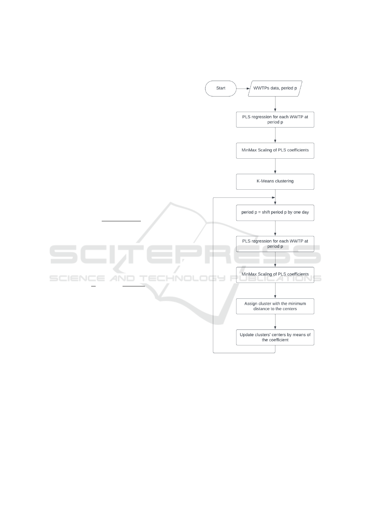
2.2.3 Implementation of Dynamic K-Means

There are four kinds of clustering (Ben

ıtez et al.,

2016): (I) static data with static number of clus-

ters, (II) static data with dynamic number of clusters

through time, (III) dynamic data with static number of

cluster and (IV) dynamic data with dynamic number

of clusters. In this case, only case (III) is considered.

First step consists in computing static K-Means

on period p. Then period p is shifted by one day.

New coefﬁcients are computed and normalised to the

reference period. The normalisation step allows the

stability of the clusters from one period to the next.

Distances between coefﬁcients and each cluster cen-

ter of the previous period are computed. WWTPs are

allocated to the nearest cluster. Then cluster centers

are updated doing the mean of new normalized coefﬁ-

cients within the clusters. Then, the process goes back

to the shifting period step and so on. Full algorithm is

depicted in Figure 1.

Figure 1: Diagram of the full WWTPs Dynamic Clustering

algorithm.

One can add a memory parameter at the centers

updating step (M

arquez et al., 2018). This allows to

smooth the impact of the previous periods. In this

case, the choice was made to omit he memory param-

eter. Indeed, information about the previous period

is already contained in the coefﬁcients since period is

only shifted by one day.

To assess Dynamic K-Means quality, adjusted-

Rand index is used in addition to Silhouette and

DB indices. Rand index is a measure of agreement

ICPRAM 2024 - 13th International Conference on Pattern Recognition Applications and Methods

664

between two consecutive partitions of Dynamic K-

Means (Rand, 1971). It is computed as:

RI =

a + b





(5)

where a is the number of WWTPs couples in com-

mon in both partitions, b is the number of couples

separated in both partitions and





refers to all pos-

sible couples. If partitions match perfectly, Rand in-

dex values 1. To ensure that random partitions will

effectively have a Rand index valuing 0, the index is

normalised by a Rand index for a random partition.

Thus, adjusted-Rand index formula is:

ARI =

RI − E[RI]

max(RI) − E[RI]

(6)

E[RI] is the expected Rand index for a random parti-

tion. By deﬁnition, max(RI) values 1.

3 RESULTS

3.1 Fitting the PLS Model

PLS Regression is computed with two target vari-

ables: energy consumption per kilogram of COD re-

moval and energy consumption per cubic meter of

treated wastewater. On average, a WWTP consumes

approximately 1 kWh/m³ of treated wastewater and 2

kWh/kg of COD removal (Stricker et al., 2018).

Which variables can provide a more comprehen-

sive explanation for consumption patterns? Vari-

ous combinations of the loading rates, suspended

solids, rainfall, temperature and pH are tested. As

in (Stricker et al., 2017), a logarithmic transforma-

tion has been previously applied to both loading rates.

Most correlated variables to the consumption per kilo-

gram of COD removal are the organic loading rate and

the suspended solids whereas for the consumption per

cubic meter of treated wastewater, it is the loading rate

of cubic meter, the rainfall and the temperature.

All PLS Regressions were trained on the whole

year 2019. COD data collection can raise missing

value. Thus, WWTPs have 48 to 363 observations in

2019. To choose among all variables, RMSE is com-

puted for each speciﬁc consumption per WWTP for

January and February 2020. Test sets have 7 to 60

observations. RMSE results are depicted in Figure 2.

The best model is the one with the lowest third

quartile of RMSE. For the energy consumption per

kilogram of COD removal, the best model is the one

using the two loading rates and the rainfall with 75%

of the RMSE under 0.35 kWh/kg of COD. For the en-

ergy consumption per cubic meter of treated wastew-

ater, the best model is the one using the two loading

rates, temperature and pH with 75% of the RMSE un-

der 0.24 kWh/m³ of treated wastewater.

However, two models seem to have the lowest

third quartile of RMSE for both speciﬁc consump-

tions. It is the one with the two loading rates only

(75% of RMSE under 0.35 kWh/kg of COD and un-

der 0.26 kg/m³ of treated wastewater) and the one

with loading rates and rainfall (75% of RMSE under

0.35 kWh/kg of COD and under 0.26 kg/m³ of treated

wastewater).

To choose between those two models, VIP are

used. Figure 3 shows the VIPs in the model using

loading rates and rainfall. One can see that the rain-

fall importance is very low. Since third quartiles of

RMSE are really closed to the model without rain-

fall and the model with less variables gives better ex-

plainability, then the selected model only uses organic

loading rate and loading rate of cubic meter.

3.2 Deﬁning the Clusters at the First

Period

K-Means clusterings are computed on 3 combina-

tions of the coefﬁcients obtained by PLS Regression.

First clustering uses all the coefﬁcients for both tar-

gets. The aim is to include all information from

the regression. The second clustering does not em-

ploy the intercepts in order to group WWTPs. Inter-

cepts are supposed less informative on the behavior

since they are output-independent. Finally, last clus-

tering only uses organic loading rate coefﬁcient to ex-

plain the consumption per kilograms of COD removal

and loading rate of cubic meter coefﬁcient to explain

the consumption per cubic meter of treated wastew-

ater. Those coefﬁcients are chosen because they are

the most correlated to their respective target variables

(Respective average Pearson Coefﬁcients are -0.8 and

-0.85). Results of those 3 clusterings are represented

in Table 2.

Table 2: Number of clusters, Silhouette and Davies-Bouldin

indices for the 3 computed clusterings.

Clustering

Silhouette

index

All coefﬁcients 0.32 1.03

Without Intercepts 0.34 0.91

Respective loading rates 0.43 0.69

The more homogeneous the formed groups are,

the closer the Silhouette index is to 1 and the DB in-

dex is to 0. The best partition is reached using the

respective loading rates of the speciﬁc consumption.

The coefﬁcients distribution for each WWTP within

the clusters is shown by Figure 4.

Detection of Energy Drifts in Waste Water Treatment Plants Using Dynamic Clustering

665

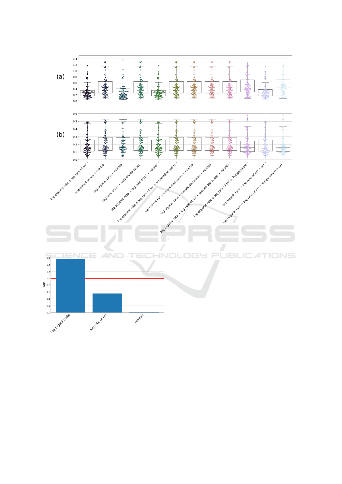
Figure 2: (a) Distribution of the RMSE in kWh/kg of COD per PLS model implemented. (b) Distribution of the RMSE in

kWh/m³ of treated wastewater per PLS model implemented.

Figure 3: VIP for each variables obtained with the models

using organic loading rate, loading rate of cubic meter and

rainfall.

One can interpret the groups as:

• Cluster 1. Consumption in kWh/kg of COD

removal increases a lot with the increase of

the organic loading rate whereas consumption in

kWh/m³ of treated wastewater rises slightly with

the increase of the loading rate of cubic meter.

• Cluster 2. Consumption in kWh/kg of COD

removal rises sharply with the increase of the

organic loading rate whereas consumption in

kWh/m³ of treated wastewater increases very

slightly with the increase of the loading rate of

cubic meter.

• Cluster 3. Consumption in kWh/kg of COD re-

moval increases very slightly with the increase of

the organic loading rate whereas consumption in

kWh/m³ of treated wastewater increases sharply

with the increase of the loading rate of cubic me-

ter.

• Cluster 4. Consumption in kWh/kg of COD re-

moval increases very slightly with the increase of

the organic loading rate whereas consumption in

kWh/m³ of treated wastewater increases sharply

with the increase of the loading rate of cubic me-

ter.

• Cluster 5. Consumption in kWh/kg of COD

removal increases slightly with the increase of

the organic loading rate whereas consumption in

kWh/m³ of treated wastewater rises very slightly

with the increase of the loading rate of cubic me-

ter.

ICPRAM 2024 - 13th International Conference on Pattern Recognition Applications and Methods

666

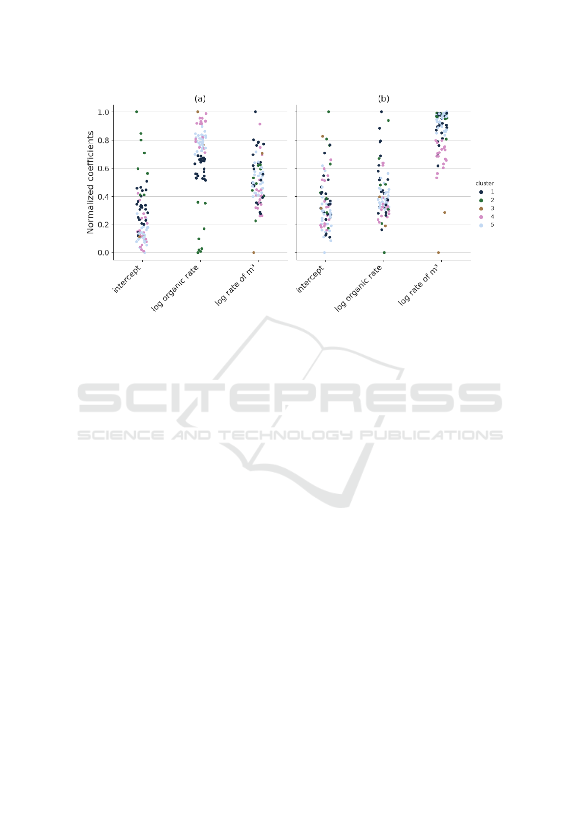
Figure 4: Distribution of the coefﬁcients per cluster. (a) Coefﬁcients for the consumption in kWh/kg of COD. (b) Coefﬁcients

for the consumption in kWh/m³ of treated wastewater.

64% of the WWTPs are in cluster 1 or cluster 5.

Those two clusters are the ones with less impact of the

inﬂuent on the consumption per cubic meter. Also,

the impact of inlet COD on consumption per kilo-

grams of COD is not extreme.

As said before, some biological processes are

known to require more energy than others (Stricker

et al., 2017). Chi-Square test between biological pro-

cess and clusters has been carried out. P-Value ob-

tained equals 1% which is under 5%. This means that

there is a relationship between biological processes

and clusters. Indeed, processes with a small footprint

such as MBR and MBBR are over represented in clus-

ter 2. Respectively, they represent 25% and 37% of

the WWTPs in cluster 2 whereas they represent 5%

of the whole sample. Those are the clusters with the

biggest inﬂuence of the organic loading rate.

3.3 Evolution of the Clusters During 3

Months

Initialization was made on the whole year before Jan-

uary 2

, 2020. From this date, Dynamic Clustering

was computed until April 1

, 2020. Movement be-

tween clusters are quantiﬁed using adjusted-Rand in-

dex, on consecutive period. If the adjusted-Rand is

not 1, then at least one WWTP has changed cluster.

Figure 5 summarized all consecutive adjusted-Rand

indices from January 2

, 2020 to April 1

, 2020.

For the ﬁrst day of Dynamic Clustering, adjusted-

Rand index does not reach 1. There is a lot of move-

ment between clusters: 57 WWTPs change cluster at

the January the 3

. This change is supposed to be the

convergence period of the Dynamic Clustering. After

January 3

, change in clusters are fewer. Clusters are

more stable. During the following shifts, 29 changes

are detected.

Figure 5 also depicts DB and Silhouette indices.

They measure clusters consistency through the dy-

namical process. Silhouette index trend is upward.

Each day, the clusters appear to become more coher-

ent. Results are not so clear regarding DB index. The

best clustering quality is reached during the month of

February.

An example of those changes during the month

of March is represented in Figure 6. Four kinds of

changes have been recorded. After January 3

, 2020,

half of the movements are between clusters 4 and

5. Those two clusters differentiate themselves by the

loading rate of cubic meter inﬂuence on energy con-

sumption. Members of cluster 5 consumption is less

inﬂuenced by the loading rate of cubic meter than

members of cluster 4.

About 30% of the changes are between clusters 1

and 5. They are characterized by a change of inﬂu-

ence in the organic loading rate on the energy con-

sumption. Members of cluster 5 consumption is less

inﬂuenced by the organic loading rate than members

of cluster 1.

Few WWTPs change clusters between 3 and 4.

Those movements show a change in the inﬂuence rate

of treated wastewater among clusters with already a

Detection of Energy Drifts in Waste Water Treatment Plants Using Dynamic Clustering

667

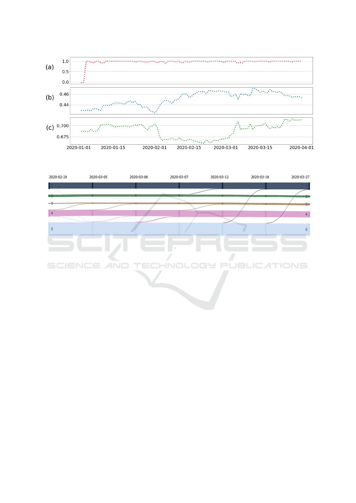
Figure 5: (a) Consecutive adjusted-Rand index between January 2

2020 and April 1

2020, (b) Silhouette Index obtained

at each step of Dynamic Clustering, and (c) DB index obtained at each step of Dynamic Clustering.

Figure 6: Recorded movements between clusters during the month of March.

higher impact of treated wastewater on energy con-

sumption.

Finally, 10% of the movements are between clus-

ters 1 and 2. Those are the two clusters with the

biggest impact of organic loading rate on energy con-

sumption. It is interesting to notice that only MBR

and MBBR processes are involved in those changes.

4 DISCUSSION AND FUTURE

WORKS

Other techniques have been explored. Namely, use of

raw data has been considered. Speciﬁc K-Means us-

ing Dynamic Time Warping have been tried (Sard

Espinosa, 2018). This technique is very computation-

ally intensive and results lead to difﬁcult-to-interpret

clusters. K-Shapes were also considered. (Yang et al.,

2017) uses K-Shapes on building energy loads. Nev-

ertheless, it is difﬁcult to introduce exogenous vari-

ables since K-Shapes are not suitable for multivariate

times series. Thus, use of raw data has been aban-

doned.

Data summary was tested with ARIMA-type mod-

els instead of regression. Those kinds of model are

classically used to summarize time series information.

For instance, (Nepal et al., 2020) applies ARIMA-

type models on building energy consumption after

clustering by day. However, this technique requires a

lot of analysis to ﬁt the data. By the way, existing au-

tomatic algorithms are not reliable and time consum-

ing. This leads to conserve the method of (Shahzadeh

et al., 2015) using Regression Coefﬁcients.

Then, relatively simple PLS Regression model

has been implemented. Further works may focus on

adding information on previous data such as lags or

moving averages. However, adding more coefﬁcients

can reduce the interpretability of results.

As speciﬁed in (Rajabi et al., 2020), K-Centroids

clustering methods are widely implemented in energy

load pattern recognition. This article focuses on clas-

sic K-Means. Yet, this technique has some limitations

like it only deals with spherical clusters, results are

subject to the randomness of the initialisation. In ad-

dition, K-Means is a hard clustering method. It is

not well suited for overlapping data points. To ﬁnd

out more, fuzzy clustering can be considered (Rajabi

et al., 2020). It can smooth the drift between two pe-

riods during the dynamical analysis. Fuzzy clustering

could be put in competition against Density-based or

Hierarchical algorithm.

ICPRAM 2024 - 13th International Conference on Pattern Recognition Applications and Methods

668

One possible extension is to move to dynamic

number of clusters. Currently, number of clusters is

ﬁxed through time. But, if each WWTP of one cluster

changes behavior, this cluster may not have any in-

terest, while a new behavior can emerge. That’s why,

moving to dynamic number of clusters could be inter-

esting.

Next step will be to detect automatically anoma-

lies during clusters changes. For instance, highlight-

ing WWTPs with constant increase of the distance to

the center. In the case of fuzzy clustering, the mem-

bership of a WWTP to a cluster can also be used.

5 CONCLUSIONS

With the aim of achieving lower CO

footprint and re-

ducing costs, treated wastewater companies improve

their energy efﬁciency. This article proposes a method

to manage those expenditures by grouping WWTPs

following their energy consumption patterns. Then,

those load patterns are analysed dynamically.

The load pattern of a WWTP is characterized by

the coefﬁcients of PLS Regression. This model ex-

plains the consumptions per kilograms of COD and

per cubic meters of treated wastewater by the two

loading rates of the plants.

The WWTPs are grouped basing on their energy

consumption behaviors by using K-Means methods.

Five distinct clusters are obtained. A majority of

WWTPs are in clusters with less impact of the loading

rate of cubic meter on consumption per cubic meters.

WWTPs with MBR or MBBR processes are over rep-

resented in clusters where the loadings of inlet COD

have a big impact on energy consumptions. As behav-

iors evolve, on average 60% of movements between

clusters are due to a change of loading rate of cubic

meter inﬂuence on energy consumption.

This method provides easily interpretable results

thanks to the employment of Regression model co-

efﬁcients. However, K-Means introduce limits. It is

a hard clustering method and it is subject to the ran-

domness of the initialisation.

Next step will be to detect anomalies during clus-

ters changes with statistical method. For instance

by analysing the evolution of the distances with the

groups centers.

ACKNOWLEDGEMENTS

We would like to thank Veolia Water France, for its

support throughout this project. We are also grateful

to the Veolia Water France for providing us the data

we needed to complete this project.

We would also like to thank our colleagues at Ve-

olia Research and Innovation for their feedback and

support during the research process.

REFERENCES

Bagherzadeh, F., Nouri, A. S., Mehrani, M.-J., and Then-

nadil, S. (2021). Prediction of energy consumption

and evaluation of affecting factors in a full-scale wwtp

using a machine learning approach. Process Safety

and Environmental Protection, 154:458–466.

Ben

ıtez, I., D

ıez, J.-L., Quijano, A., and Delgado, I.

(2016). Dynamic clustering of residential electric-

ity consumption time series data based on hausdorff

distance. Electric Power Systems Research, 140:517–

526.

Borzooei, S., Miranda, G. H. B., Abolfathi, S., Scibilia,

G., Meucci, L., and Zanetti, M. C. (2020). Appli-

cation of unsupervised learning and process simula-

tion for energy optimization of a WWTP under vari-

ous weather conditions. Water Science and Technol-

ogy, 81(8):1541–1551.

Davies, D. and Bouldin, D. (1979). A cluster separation

measure. Pattern Analysis and Machine Intelligence,

IEEE Transactions on, PAMI-1:224 – 227.

Geladi, P. and Kowalski, B. R. (1986). Partial least-squares

regression: a tutorial. Analytica Chimica Acta, 185:1–

17.

Harrou, F., Cheng, T., Sun, Y., Leiknes, T., and Ghaffour, N.

(2021). A data-driven soft sensor to forecast energy

consumption in wastewater treatment plants: A case

study. IEEE Sensors Journal, 21(4):4908–4917.

ISO 50001 (2018). Syst

emes de management de l’

energie

— Exigences et recommandations pour la mise en

oeuvre. Standard, Organisation Internationale de Nor-

malisation, Geneva, CH.

Li, Z., Zou, Z., and Wang, L. (2019). Analysis and fore-

casting of the energy consumption in wastewater treat-

ment plant. Mathematical Problems in Engineering,

2019:8690898.

arquez, D. G., Otero, A., F

elix, P., and Garc

ıa, C. A.

(2018). A novel and simple strategy for evolving pro-

totype based clustering. Pattern Recognition, 82:16–

30.

Nepal, B., Yamaha, M., Yokoe, A., and Yamaji, T. (2020).

Electricity load forecasting using clustering and arima

model for energy management in buildings. Japan Ar-

chitectural Review, 3(1):62–76.

Qiao, J. and Zhou, H. (2018). Modeling of energy consump-

tion and efﬂuent quality using density peaks-based

adaptive fuzzy neural network. IEEE/CAA Journal of

Automatica Sinica, 5(5):968–976.

Rajabi, A., Eskandari, M., Ghadi, M. J., Li, L., Zhang, J.,

and Siano, P. (2020). A comparative study of clus-

tering techniques for electrical load pattern segmen-

Detection of Energy Drifts in Waste Water Treatment Plants Using Dynamic Clustering

669

tation. Renewable and Sustainable Energy Reviews,

120:109628.

Rand, W. M. (1971). Objective criteria for the evaluation of

clustering methods. Journal of the American Statisti-

cal Association, 66(336):846–850.

Rousseeuw, P. J. (1987). Silhouettes: A graphical aid to

the interpretation and validation of cluster analysis.

Journal of Computational and Applied Mathematics,

20:53–65.

Sard

a-Espinosa, A. (2018). Comparing time-series cluster-

ing algorithms in r using the dtwclust package.

Shahzadeh, A., Khosravi, A., and Nahavandi, S. (2015).

Improving load forecast accuracy by clustering con-

sumers using smart meter data. In 2015 International

Joint Conference on Neural Networks (IJCNN), pages

1–7.

Silva, J., Faria, E., Barros, R., Hruschka, E., de Carvalho,

A., and Gama, J. (2014). Data stream clustering: A

survey. ACM Computing Surveys, 46.

Stricker, A.-E., Husson, A., and Canler, J.-P. (2017).

Consommation

energ

etique du traitement intensif des

eaux us

ees en france :

etat des lieux et facteurs de vari-

ation. Technical report, Irstea centre de Bordeaux, 50,

avenue de Verdun 33612 Cestas cedex.

Stricker, A.-E., Husson, A., and Canler, J.-P. (2018).

Consommations

energ

etique des stations d’

epuration

franc¸aises,

Etat des lieux et recommandations. Tech-

nical report, Irstea centre de Bordeaux, 50, avenue de

Verdun 33612 Cestas cedex.

Syakur, M., Khusnul Khotimah, B., Rohman, E., and

Dwi Satoto, B. (2018). Integration k-means cluster-

ing method and elbow method for identiﬁcation of the

best customer proﬁle cluster. IOP Conference Series:

Materials Science and Engineering, 336:012017.

Vancoken, S. (2004). La r

egression PLS. Groupe de Statis-

tique, Universite de Neuch

atel.

Wang, Y., Chen, Q., Kang, C., and Xia, Q. (2016). Clus-

tering of electricity consumption behavior dynamics

toward big data applications. IEEE Transactions on

Smart Grid, 7(5):2437–2447. Cited By :187.

Xia, X. (2013). The Study of a Class of the Brownian

Derivative System. International Journal of Differ-

ential Equations and Applications, 12(1).

Yang, J., Ning, C., Deb, C., Zhang, F., Cheong, D., Lee,

S. E., Sekhar, C., and Tham, K. W. (2017). k-shape

clustering algorithm for building energy usage pat-

terns analysis and forecasting model accuracy im-

provement. Energy and Buildings, 146:27–37.

ICPRAM 2024 - 13th International Conference on Pattern Recognition Applications and Methods

670