Comparison Between Graph Databases and RDF Engines for Modelling

Epidemiological Investigation of Nosocomial Infections

Lorena Pujante-Otalora

, Manuel Campos

1,2

, Jose M. Juarez

and Maria-Esther Vidal

MedAILab, Department of IT and Systems, University of Murcia, Campus Espinardo, Murcia, 30100, Spain

Murcian Bio-Health Institute, IMIB-Arrixaca, El Palmar, Murcia, 30120, Spain

Leibniz University of Hannover and L3S Research Center and TIB Leibniz Information Centre for Science and

Technology, Hannover, Germany

Keywords: Graph Database, Knowledge Graphs, Epidemiology, Benchmark, Neo4j, GraphDB.

Abstract: We have evaluated the performance of property and knowledge graph databases in the context of

spatiotemporal epidemiological investigation of an infection outbreak in a hospital. Specifically, we have

chosen Neo4j as graph database, and GraphDB for knowledge graphs defined following RDF and its extension

RDF*. We have defined a domain model describing a hospital layout and patient movements. For

performance comparison, we have created ten graphs with different sizes based on MIMIC-III, implemented

three epidemiological queries in Cypher, SPARQL and SPARQL* and defined three benchmarks that measure

the execution time and main memory consumption of the three queries in each graph and database engine.

Our research suggests that query complexity is a more determinant factor than graph size in the performance

of the query executions. Neo4j presents better times and memory consumption than GraphDB for simple

queries, but GraphDB is more efficient when traversing big subgraphs. Between RDF and RDF*, RDF* offers

a more compact and human-friendly modelling and a better performance of the query execution.

1 INTRODUCTION

In recent years, we have witnessed an exponential

growth in data to be stored and processed at any area,

what is called “big data”. This vast amount of data

with no rigid schemes and generally stored across

multiple machines promoted some new type of

databases, encompassed in the term NoSQL

databases (Leavitt, 2010). Graph databases are

NoSQL databases that represent data as property

graphs, providing an efficient storage and

management of highly interconnected data. The

interest in modelling data as property graphs has

increased in recent years due to their advantages in

network analysis and the semantic web. Related to

this context, we also find knowledge graphs, a

semantic web technology that links massive and

cross-domain data used on tasks like information

retrieval, hidden linkage identification, and

knowledge-driven decision support (Li et al., 2022).

Unlike graph databases, which present different

strategies to model the internal representation of the

graphs, knowledge graph databases usually represent

data as a set of triples in the form of <subject,

predicate, object> following RDF (Resource

Description Framework).

In the field of medicine and healthcare, both

property and knowledge graphs are increasingly used

in tasks such as validation of diagnoses (Gu et al.,

2022; Yin et al., 2021), prediction of patient clinical

pathways (Trevena et al., 2022), suggestions of

treatment plans(LIU et al., 2022) and drugs (Rivas &

Vidal, 2021) and integration of heterogeneous

healthcare data and electronic health records for a

common storage (Freedman et al., 2020) and its

interoperability (Kiourtis et al., 2019). We think a

graph can be a valuable tool for modelling a hospital

and the patients’ movements during their stays. Thus,

we could examine the connections between patients

and medical staff through the hospital layout over

time. In (Pujante-Otalora et al., 2023), we studied

how graphs are used in spatiotemporal

epidemiological research.

In this paper, we empirically evaluate the

performance of property and knowledge graphs to

solve spatio-temporal queries that correspond to tasks

of the epidemiological research of hospital infectious

outbreaks. In particular, the knowledge graphs are

Pujante-Otalora, L., Campos, M., Juarez, J. and Vidal, M.

Comparison Between Graph Databases and RDF Engines for Modelling Epidemiological Investigation of Nosocomial Infections.

DOI: 10.5220/0012319900003657

Paper published under CC license (CC BY-NC-ND 4.0)

In Proceedings of the 17th International Joint Conference on Biomedical Engineering Systems and Technologies (BIOSTEC 2024) - Volume 2, pages 23-36

ISBN: 978-989-758-688-0; ISSN: 2184-4305

based on triples and delimited by RDF 1.1 (RDF 1.1

Concepts and Abstract Syntax, n.d.) and its extension

RDF* (RDF-Star and SPARQL-Star, n.d.). To this

aim, we have designed a domain model for hospitals

focused on spatially and temporally describing the

patients' movements during their stay. We have also

generated graphs of different sizes, taking as a source

the freely-available database MIMIC-III (Johnson et

al., 2016), which comprises information about

patients admitted to critical care units at a large

tertiary care hospital. We have chosen Neo4j as the

graph database engine for the property graphs and

GraphDB for the knowledge graphs. For the

evaluation, three queries that represent three tasks

from the epidemiological research process have been

defined and implemented in Cypher -Neo4j query

language-, SPARQL 1.1 (SPARQL Protocol and RDF

Query Language)(SPARQL 1.1 Query Language,

n.d.) and its extension SPARQL*. These queries can

be defined as reachability and pattern-matching

graph-based tasks and have different levels of

complexity (number of required and optional paths,

length of the paths, number and type of the variables

to retrieve). Finally, we discuss the results of our

evaluation and outline the different conditions that

benefit the studied engines.

To summarize, our contributions are as follows:

i) Design of a domain model that describes a

hospital layout and the movements of the

inpatients as a log of all their events.

ii) Description of three epidemiological

research queries in terms of graph tasks and

their paths.

iii) An empirical study of the performance of

property graphs and knowledge graphs

based on the queries.

This paper is organised as follows: Section 2

summarizes related works. Section 3 describes the

graph database engines (Section 3.1), the domain

model (Section 3.2), the queries (Section 3.3), the

datasets (Section 3.4), the storage use (Section 3.5)

and the benchmarks (Section 3.6). Experimental

results and their discussion are in Section 4.

Conclusions are in Section 5.

2 RELATED WORK

In the past few years, several works that aim to

compare graph databases and knowledge graph

databases have been published. These comparisons

focus on the performance of the database, mainly

measured as the execution time of a set of queries that

address different graph tasks (adjacency, reachability,

pattern matching, shortest path, etc.) over real-world

or synthetic datasets of various sizes. The graph tasks,

the query strategy and the datasets affect the results

of the studies. (Hohenstein & Jergler, 2019) studied

fairness in the most applied methods in graph

database comparisons.

These comparative works often focus solely on

property or knowledge graph databases. In the case of

knowledge graph databases, GraphDB and Stardog

are among the RDF engines that appear the most and

with the best results. (Atemezing & Amardeilh, 2018)

studied the bulk loading, scalability and query

execution time of four RDF engines (GraphDB,

Oracle 12c, Stardog, Virtuoso) over two real-world

datasets from the EU Publications Office. (Bellini &

Nesi, 2018) compared the execution time of a set of

ten RDF engines against a Smart City RDF

Benchmark dataset.

In the case of graph databases, Neo4j is

commonly compared, presenting promising results.

(Wang et al., 2020) compared three graph databases

(Neo4j, TigerGraph, TuGraph) against some

synthetic social networks. (Ferro & Sinico, 2018)

compared three graph databases (ArangoDB, Neo4j,

OrientDB) and a relational database (PostgreSQL)

against a dataset based on an Italian Business

execution time and RAM and CPU usage of four

graph databases (JanusGraph, Nebula Graph, Neo4j,

TigerGraph) against data from the LDBC Social

Network Benchmark

0F0F.

Works that compare graph databases with RDF

engines are less common. (Kovács et al., 2019)

compared the execution times of two graph databases

(Neo4j, JanusGraph) with an RDF engine

(Blazegraph) using a dataset loaded with information

from Wikidata. (Li et al., 2022) compared the

execution time of four triple stores (GraphDB,

Virtuoso, RDF4j, Fuseki) with a graph database

(Neo4j) and an Ontology-Based Data Access

database (Ontop) against a dataset of topological data.

Our work differs from this last one in that their

queries represent geometrical operations for spatial

analysis of polygons based on points, while our

spatial representation of a hospital is based on relative

relations (next to, opposite, inside) of its architectural

elements (room, corridor, floor). Besides, we consider

the temporal dimension.

HEALTHINF 2024 - 17th International Conference on Health Informatics

3 DATA AND METHODS

3.1 Graph Database and RDF Engine

Neo4j is a database engine that relies on labelled

property directed multigraphs, which are

implemented in native structures. That is, the

underlying structure of the database has been

designed to store data in the form of nodes and edges.

Neo4j presents a schema-less and implements its own

query language, Cypher. It provides an API REST

and official drivers for several programming

languages.

GraphDB is a graph database used to store and

manage knowledge graphs that can perform semantic

inferencing. It is fully compliant with RDF 1.1 and

SPARQL 1.1, and it is one of the few commercial

graph databases that entirely supports their extensions

RDF* and SPARQL*. GraphDB implements the

RDF4J framework interfaces in pursuit of

compatibility with RDF serialization formats and

easy application integration. GraphDB offers an

official API REST for administration tasks but not

querying the database.

It is noteworthy that both databases are

implemented in Java. Some newer graph databases

implemented in C++ (e.g., TigerGraph) may offer

faster results.

3.2 Domain Model

Our model aims to represent patients’ movements

during their hospital stay. This model focuses on both

the temporal and the spatial dimensions. The spatial

dimension consists of a hierarchy of locations that

goes from bed to building, passing through rooms,

corridors, areas and floors. There are also spatial

relations between some locations of the same level in

the hierarchy, such as being next to or opposite some

other location. For example, a room can be next to

another, but not opposite a corridor. The spatial

dimension also covers the hospitalization units and

services that care for the patients during their stay.

The locations form the physical spatial dimension,

and the units and services are the logical spatial

dimension. For the temporal dimension, there is a log

with the hospital episodes of each patient, where each

episode represents an hospital stay and consists of a

set of all its events. An event represents any

movement of the patient in the hospital (a stay in a

room, a surgical operation, taking radiography, etc.)

or other actions, such as getting the results of a

microbiological test. Each episode and event has a

start and end date and time. Events may occur in a

time moment (both dates and times will be the same)

or interval. Some of them are connected to a location,

so they are the union point between temporal and

spatial dimensions. Events can also be connected to

the hospitalization units that cared for the patient.

In the model, some relations have properties. That

is the case of all the relations from the spatial

dimension, which have a weight to represent how

close the two locations are. The relation that connects

a microbiological test with the microorganism found

also has a property to mark if the microorganism is

multidrug-resistant. The right side of Figure 1 shows

the entire domain model. Given the lack of detailed

information on the dataset about the hospital layout

and what happened during the hospitalizations, we

have used a reduced version of the domain, shown on

the left side of Figure 1. The explanation of the

complete model is out of the scope of this work.

The implementation of our domain model differs

from property graph to knowledge graph. Neo4j

presents a schema-less model where nodes and edges

can belong to one or several classes that act like labels

since they do not restrict the number and datatype of

the properties of its nodes and edges. Moreover, nodes

and edges hold their own information in the form of

properties. When translating the domain model to an

RDF ontology, we find that it is an abstract

representation that does not differentiate data from

metadata since it is based on the concept of statement:

a triple made of a subject, a predicate and an object.

The subject denotes a resource defined by a URI

(Uniform Resource Identifier), and the predicate

denotes a property or relation of the subject. The object

is the value of the data property or the URI of another

resource (the subject of one statement can be the object

of another). The class (or classes) of a resource is also

the object of a statement. In a graph representation,

subjects and objects would be the nodes, and predicates

would be the edges between them.

A significant difference between a Neo4j graph

and an RDF knowledge graph is how implement

edges with properties. In RDF it is not possible to

make a statement where an edge is a subject. There

are four approaches to solve this problem: standard

reification, n-ary relations, singleton properties and

named graphs. We have chosen standard reification,

which consists in creating a new class to represent the

edges as resources (nodes), making possible

statements that have them as subjects and their data

properties as objects. On the other hand, RDF* allows

making statements about other statements. So it is

possible to define a statement that represents that two

resources are linked, which is the subject of another

statement that adds a property to the relation.

Comparison Between Graph Databases and RDF Engines for Modelling Epidemiological Investigation of Nosocomial Infections

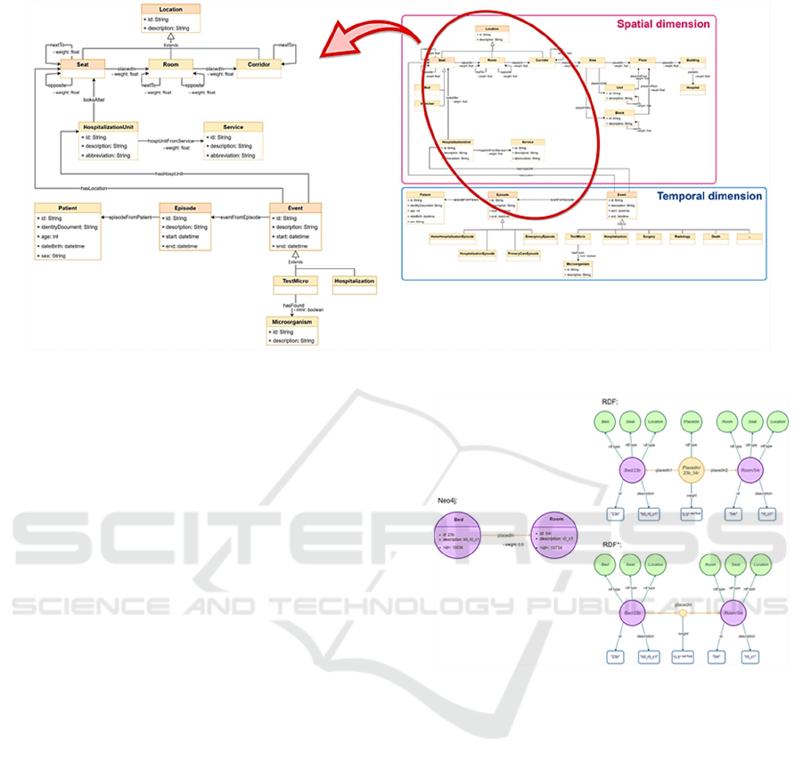
Figure 1: Domain model.

Figure 2 shows a graphical representation in each

data model of the edge placedIn between a Bed and a

Room, which has the property weight. From here on,

we will refer to Neo4j nodes and RDF and RDF*

resources as “nodes of individuals” and to the nodes

with the name of the classes and the value of the data

properties as “nodes of literals”.

3.3 Query Definition

We defined three queries representing relevant

clinical tasks for detecting and studying an infection

outbreak. All these queries could be described as

reachability and pattern-matching graph-based tasks,

where the paths are temporarily and semantically

conditioned. Tables 1, 2 and 3 show the description

and characteristics of every query. Figure 3 shows a

schematic representation of each query. Each query is

defined by the following characteristics:

• A general description of the query as a graph-

based task.

• Number of required and optional paths, where

“required” means that the path must match with

the data and “optional” means that it is not

mandatory that all of these paths match, but at

least one must do it.

• Tentative number of steps (number of traversed

edges) that each path should have in a

pseudocode version of the query defined

directly over the domain model diagram. When

translated to Cypher, SPARQL and SPARQL*,

these paths and their length may change.

Figure 2: Graphical representation of the relation placedIn

between two nodes Bed and Room with their properties. In

Neo4j nodes, <id> property is an internal identifier. In

RDF* representation, the small yellow node symbolises the

statement that links the purple nodes and on which a new

statement is added to link to it the weight property.

3.4 Dataset Characteristics

We have generated ten graphs of different sizes from

MIMIC-III. We have used admissions and transfers

tables to get the stays and ward movements of the

patients, services table to get the services responsible

for the patients and microbiologyevents table to get

their positive microbiological tests.

Since the information provided by MIMIC-III

only partially covers the classes and relations of our

domain model, we have extended it by creating a

fictitious hospital with a simple layout.

In the physical spatial dimension, MIMIC-III

works with wards. For each ward, we have created a

HEALTHINF 2024 - 17th International Conference on Health Informatics

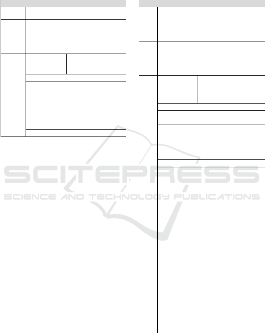
Table 1: Description of Query 1.

Query 1 (Q1)

Clinical

task

Outbreak detection.

Description

Given a Service and a Microorganism,

find all the Patients hospitalised under

that Service who had an infection of the

given Microorganism. The search is

within a time interval.

Characteristics

Graph-based

task

Find the nodes that

are the union points

between two nodes.

Required paths: 2

Description

Number of

steps

- From the given

Microorganism to

connected Patients

- From the given Service

to connected Patients

Optional paths: 0

set of rooms with a maximum of ten beds. There must

be sufficient beds in each ward to encompass the

maximum number of simultaneous hospitalised

patients if we compacted all its hospitalisations in just

one year. Then, these beds are homogenously

distributed between the rooms.

We organised the rooms into four groups

(surgical, medical, mixed and neonatal) according to

the type of service that attends the most

hospitalisations in their wards. All the rooms are

located on a single floor and distributed in two

parallel main corridors. These corridors are divided

into several shorter corridors, each with a maximum

of twenty rooms. Our fictitious hospital has 156

Surgical rooms with 1,413 beds, 23 Medical rooms

with 179 beds, 56 Mixed rooms with 510 beds and 4

Neonatal rooms with 13 beds. Figure 4 is a schematic

representation of the hospital layout where we can see

the four groups of rooms and their distribution. For

the logical spatial dimension, we have added to each

service several hospitalization units, such that no

hospitalization unit attends more than 1,500

hospitalisations.

Note that the specific design for this example did

not impact the resolution of the queries, and other

distributions would be possible since the data model

allows for more complex designs while the classes

used are the same.

To evaluate the scalability of the queries at the

maximum extent with the data available, it is

necessary to generate graphs of different sizes. We

generated every graph to comprise the whole MIMIC-

Table 2: Description of Query 2.

Query 2 (Q2)

Clinical

task

Outbreak detection from the index patient.

The index patient is the first patient that

catches the attention of the researchers.

This patient may not be the first person

infected.

Description

Given a Patient and a Microorganism, find

all the Patients spatially connected with

them and who had an infection of the given

Microorganism. The search is within a time

interval.

Characteristics

Graph-based

task

Find all the connected

nodes to two nodes

through some specific

paths.

Required paths: 2

Description

Number

of steps

- From the given Patient to all

the Seats they have been

- From the Patients found in

the optional paths to the given

Microorganism

Optional paths: 6

Description

Number

of steps

- From the Seats to their

connected Locations via

placedIn until Area

1-3

- From the Rooms to other

adjacent Rooms

- From the Areas to other Areas

belonging to the same Logic

zone (group of areas, not

necessarily contiguous, with

some common characteristics)

- From all the Locations found

in the previous paths to their

connected Seats

1-3

- From the Seats of the

previous path to their

connected Patients

- From the Events of the given

Patient to the Hospitalization

Units that cared for them.

Then, from these

HospitalizationUnits to other

connected Patients

III dataset in one year and then picked sets of events

(with their linked episodes, patients and

microorganisms) such that it goes from around

Comparison Between Graph Databases and RDF Engines for Modelling Epidemiological Investigation of Nosocomial Infections

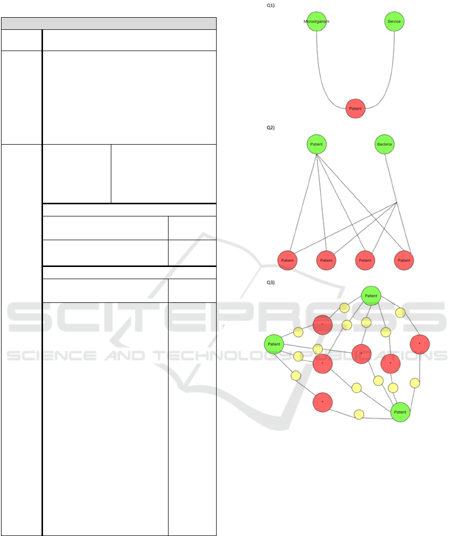
Table 3: Description of Query 3.

Query 3 (Q3)

Clinical

task

Investigation of contagion sources

Description

Given a set of Patients and a period of

time, find the shared Locations,

Hospitalization Units, Services and

Microorganism between them. That is,

we want to find what connects

patient_1 with patient_2, patient_1 with

patient_3, patient_2 with patient_3,

etcetera.

Characteristics

Graph-based

task

Find the nodes that are

the union points

between a given set of

nodes through some

specific paths.

Required paths: 1

Description

Number

of steps

From the given Patients to

all their Events

Optional paths: 6

Description

Number

of steps

- From each Event to every

other Event passing through

their:

• shared Hospitalization

unit.

• shared Service.

• shared Locations. That

is, first from the Event to

its connected Seat and

from this to its higher-

level Locations, and

then the inverse path.

2-8

• shared Locations,

through Logic zone.

• adjacent Rooms.

- From each TestMicro to

every TestMicro passing

through their shared

Microorganisms.

25,000 events up to 475,000 events in MIMIC-III

with successive increments of 50,000 events.

In total, we have ten graphs called G1 to G10,

being G1 the smaller and G10 the bigger. The hospital

layout and number of hospitalization units and

services are the same in all the graphs. Hence, there

is a different density of events per location.

Figure 3: Schematic representation of each query. Green

nodes represent the initial nodes given as a parameter, and

red nodes represent the result nodes after traversing the

defined required and optional paths, represented with the

black lines. In the case of Q3, red nodes have an asterisk

because they can be of any class since they are the union

between some initial nodes. Yellow nodes represent all the

nodes of the traversed paths, which are returned with the

red ones.

Table 4 shows for each graph the number of nodes

of the classes that most significantly impact the

execution of the queries. These are the most

numerous classes, and their nodes are often the start

or end of the queries or a connection between paths.

Table 5 shows the main “general graph features” of

each graph, differentiating between each graph

representation.

HEALTHINF 2024 - 17th International Conference on Health Informatics

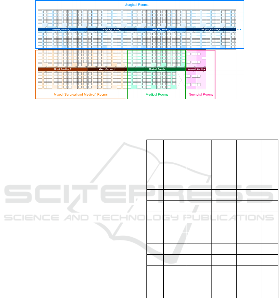
Figure 4: Schematic representation of our MIMIC-III hospital room layout. To simplify this figure, each corridor (except

Neonatal_Corridor) has half the number of rooms actually assigned, and only a portion of the Surgical corridors are shown.

Regarding the specific domain, a big hospital in

Spain would be the Complex University Hospital of La

Coruña in Galicia with about 1,300 beds. It registers

about 37,000 admissions yearly according to the

National Institute of Statics of Spain. This number is

near the 38,000 patients in the most extensive graph.

3.5 Storage Use

Concerning the disk space required to store the

graphs, we have observed a noteworthy difference

between Neo4j and GraphDB, which could be critical

for the scalability of large graphs. To optimise the data

storage, Neo4j uses linked lists of fixed-size records to

store each data type (nodes, edges, properties).

GraphDB combines an entity pool (files where all the

entities -URIs, literals, RDF* triples- are stored as 32-

bit or 40-bit internal IDs) with two main indexes,

subject-predicate index and predicate-object index.

Figure 5 shows how much disk space each graph

needs to be stored in each database engine. As

expected, the implementations in RDF* of the graphs

are a bit lighter than in RDF. The difference between

these two technologies goes between 6.2% and 14.4%

and increases with the size of the graph. It is worth

mentioning that each database usually represents an

increase of about 55 MB in RDF and RDF*. In Neo4j,

this increase goes from 5 MB in the last graphs to 12

MB in the first ones.

An interesting side finding was that although the

number of nodes and edges has been multiplied by 17,

the size to store the graphs has only been increased

around 7 times in RDF and 6.5 times in RDF*. In

contrast, G10 is 20 times bigger than G1 in Neo4j.

These findings could suggest that future studies

would need to analyse at which point graphs stored in

Neo4j are bigger than in GraphDB.

Table 4: Classes with a high impact on the execution of the

queries.

Graph

# Patients

# Events

# Events with

Location

# TestMicro

# Microorganisms

G1 1,903 25,050 8,054 16,722 135

G2 5,702 75,039 24,612 49,560 197

G3 9,028 125,200 39,458 84,351 219

G4 14,027 173,307 61,862 109,379 227

G5 14,114 225,214 63,139 159,633 257

G6 15,471 275,625 71,090 201,674 288

G7 17,244 324,776 77,864 243,646 298

G8 20,032 375,211 89,471 281,996 303

G9 27,276 425,141 122,393 298,212 304

G10 38,066 474,922 169,435 299,870 304

3.6 Benchmark Characteristics

In this work, we analysed the performance of the

database engines when executing the queries defined.

We set two representative measures:

• Execution Time: it represents the time

between sending the query request to the

API and receiving its answer.

• Maximum Main Memory: it is the amount of

main memory required to execute the task.

We got the maximum main memory by

Comparison Between Graph Databases and RDF Engines for Modelling Epidemiological Investigation of Nosocomial Infections

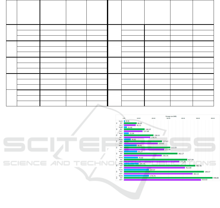
Table 5: General graph features. RDF and RDF* are deployed in GraphDB. The numbers are represented in thousands.

Graph

Database

Engine

# Nodes of

individuals

# Nodes

literals

# Edges

Graph

Database

Engine

# Nodes of

individuals

# Nodes

literals

# Edges

Neo4j 31 0 66

Neo4j 312 0 643

RDF 54 49 230 RDF 519 431 2,286

RDF* 31 49 208 RDF* 312 431 2,079

Neo4j 90 0 186

Neo4j 365 0 750

RDF 145 134 648 RDF 614 495 2,689

RDF* 90 134 593 RDF* 365 495 2,440

Neo4j 148 0 305

Neo4j 422 0 866

RDF 238 215 1,064 RDF 710 566 3,107

RDF* 148 215 974 RDF* 422 566 2,819

Neo4j 208 0 430

Neo4j 490 0 1,008

RDF 323 303 1,473 RDF 793 663 3,544

RDF* 208 303 1,358 RDF* 490 663 3,240

Neo4j 260 0 534

G10

Neo4j 565 0 1,168

RDF 425 362 1,885 RDF 870 774 3,997

RDF* 260 362 1,720 RDF* 565 774 3,692

using a background process that measures

the main memory consumption of the

database engine while the query is running.

Then, we pick the maximum value.

From here on, we will refer to the execution time

as “time” and to the maximum main memory

consumption as “memory”.

We have configured three benchmarks to study the

performance of Neo4j and GraphDB. Each

benchmark evaluates one of the proposed queries in

the ten graphs (G1, G2…). For each graph, we have

defined 12 sets of values representing each month of

the year. These 12 sets are requested three times.

Then, we calculated the mean of the time and memory

values.

For each query, we have selected the patient,

microorganism or service that is in the third quartile

of the nodes of its class with more connections. In

queries requiring a set of patients, we always used 15.

These patients have been chosen randomly between

those with more connected patients than the third

quartile. We consider that 15 is a high enough number

to represent a significant outbreak.

To ensure that cache memory is not preserved

between different processes, each query request is

executed in cold cache.

Regarding the execution features, we have

worked with Neo4j CE 4.4.18 and GraphDB Free

10.2.0. We have implemented all the queries in

Cypher, SPARQL and SPARQL*. The requests have

been made locally. For the communication with the

Figure 5: Storage size of each graph on each database

engine.

databases we have used Neo4j Python Driver(Neo4j

Python Driver, 2023)

1F1F for Neo4j and

SPARQLWrapper(SPARQLWrapper, 2022)2F2F Python

library for GraphDB. The experiments were run on a

PC with an Intel i9-12900K, 16GB RAM and 1TB

M2 drive, running a 64-bit Linux Ubuntu 22.04.

4 EXPERIMENTAL RESULTS

AND DISCUSSION

4.1 Query 1

Q1 consists of the intersection of two short required

paths with a fixed length. It can be observed in

Figures 6a and 6b that Neo4j performs better in time

HEALTHINF 2024 - 17th International Conference on Health Informatics

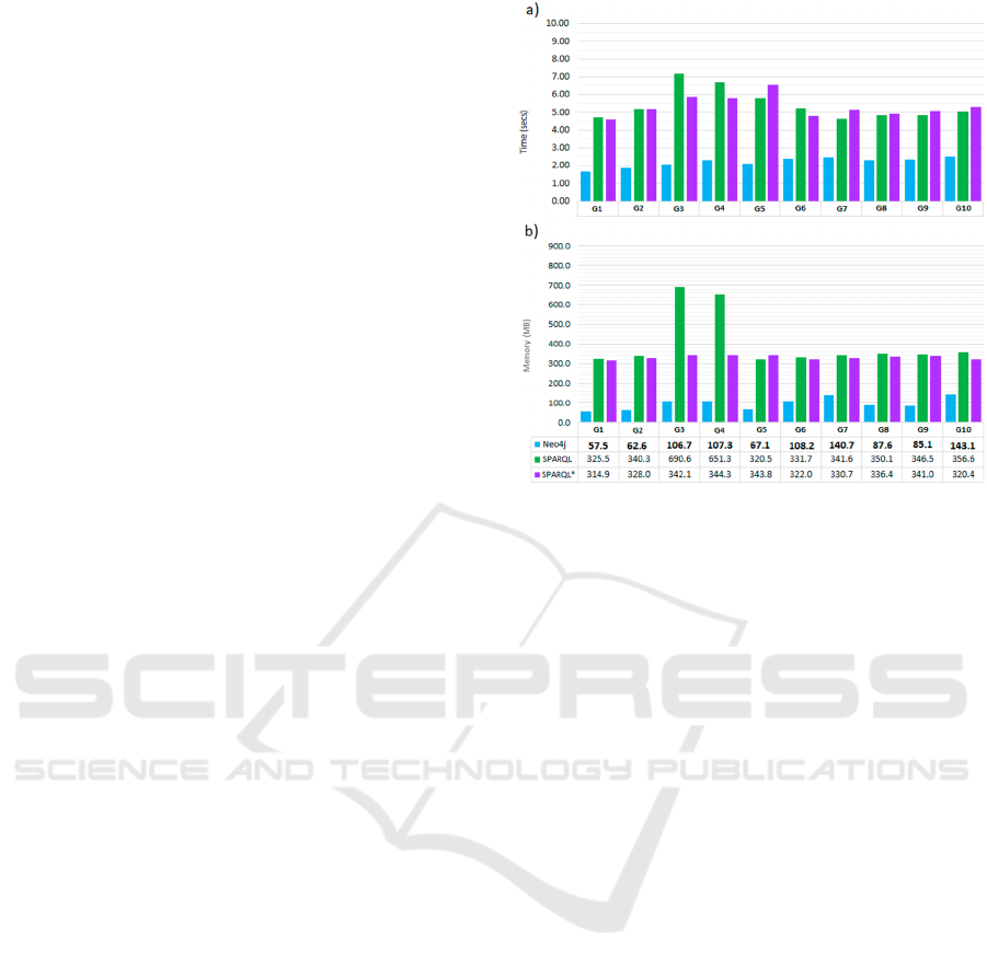
and memory in all the graphs. Another finding is that

SPARQL* requires a less time and memory than

SPARQL for almost all the graphs.

We can also observe that both the time and the

memory remain stable for all the graphs even though

the proportions of TestMicro per Microorganism and

Events per Service increased significantly. The only

exception is found in G3 and G4, where the memory

in SPARQL doubles that of the rest of the graphs. This

exception will be present in the rest of the queries and

might be related to a change in the query schedule,

which can be corroborated by the curves depicted by

the time series in SPARQL and SPARQL*. They

grow slightly and stay higher until G5, then descend,

and finally remain stable until the last graph.

The time behaviour of the three engines can be

explained if we assume that the number of results

(Patient nodes) of a query is related to the number of

edges and nodes traversed. For each Patient node, it

is necessary to traverse a path to its connected

Microorganism nodes and other path to its connected

Services. For example, if none of the Microorganism

nodes is the requested one, then the paths to the

Service nodes will not be traversed.

In Table 6, we have calculated for every graph the

average number of results (number of distinct Patient

nodes returned) for each month's set. Then, we have

divided it between the average time of Q1 in that

graph to measure how much time is needed to get a

result. This table shows that the number of results

does not increase with the graph’s size (total number

of nodes and edges) and that the time per result

depicts similar curves to the execution time.

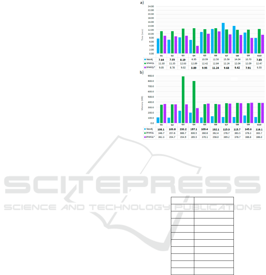
4.2 Query 2

Q2 is a query that traverses a complete tree from a

Patient node to all the Patient nodes connected with

it through some optional paths over the entire domain

model. Note that the proportions of Events per Bed

and Events per HospitalizationUnit are high and

increase in each graph, implying an “explosion” of

paths to traverse. Thus, Q2 is a suitable query to

understand better how the engines behave when

traversing large subgraphs.

The period used as a parameter in the query is 30

days, which is a period even larger than the usually

considered in the initial investigation of an outbreak.

Figures 7a and 7b show the time and memory of

executing Q2. Regarding time, SPARQL and

SPARQL* are faster than Neo4j (except for the three

Figure 6: Comparison of Neo4j, SPARQL and SPARQL*

for Q1 executions in the graphs G1 to G10. a) Execution

time comparison in seconds. b) Maximum main memory

consumption comparison in MB. In memory chart, for

every graph the smallest value is marked in bold.

most minor graphs), and the difference grows with the

size of the graphs. If we observe Neo4j time, we can

differentiate two rises. The first one goes from G1 to

G5. The second one starts on G7 and does not seem

to have a maximum nearby.

We have calculated the average time per result as

in Q1, where results are the Patient nodes connected

to the starting one. The results are in Table 7, where

we can see that the time curves also happen in the

time per result series. But note that in the first hill, the

time per result grows with the number of results,

while in the last rise, the number of results remains

around 40, and the time per result only increases. We

suspect that from G5 to G7, there must be a change in

the strategy selected by the query scheduler.

In SPARQL and SPARQL*, time and memory

present curves with similar shapes and values to those

we got in Q1. Table 7 shows two similar behaviours

in the average time per result whose start and end

graphs coincide. This fact supports the supposition

that the query scheduler of GraphDB starts to change

the strategy with graphs with a size similar to G4

(around 500,000 nodes and 1,300,000 edges), and this

change is effective when the graph has a size similar

to G6 (around 1,000,000 nodes and 2,000,000 edges).

Comparison Between Graph Databases and RDF Engines for Modelling Epidemiological Investigation of Nosocomial Infections

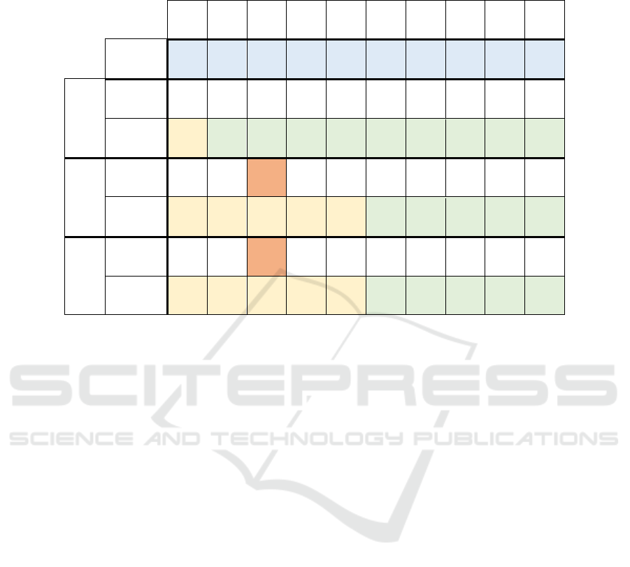
Table 6: Comparison of Neo4j, SPARQL and SPARQL * for Q1 executions in the graphs G1 to G10 of the average time to

get a result. We also show the average time of the query in each graph (Figure 6-a). We have marked the groups of

neighbouring graphs with similar behaviour in yellow and green. We have also marked the time relative maximum in orange.

G1 G2 G3 G4 G5 G6 G7 G8 G9 G10

Avg

#Results

14 25 26 31 34 38 36 36 37 38

Neo4j

Avg time

(secs)

1.69 1.85 2.07 2.29 2.09 2.40 2.47 2.30 2.33 2.50

AvgTime/

AvgRes

0.12 0.07 0.08 0.07 0.06 0.06 0.07 0.06 0.06 0.07

SPARQL

Avg time

(secs)

4.73 5.19

7.16 6.68 5.77 5.21 4.62 4.82 4.83 5.04

AvgTime/

AvgRes

0.33 0.21 0.28 0.22 0.17 0.14 0.13 0.13 0.13 0.13

SPARQL *

Avg time

(secs)

4.59 5.19

5.88 5.80 6.55 4.78 5.15 4.91 5.08 5.31

AvgTime/

AvgRes

0.32 0.21 0.23 0.19 0.19 0.13 0.14 0.14 0.14 0.14

4.2.1 Query 2: Version that Returns the

Solution Paths

Given the aim of Q2, it could be interesting that in

addition to the Patient nodes, it also returned the

traversed paths from the starting Patient to the Patient

nodes in the tree’s leaves. We have defined a modified

version to return the effective paths so we can study

if “saving” the paths along the query execution

implies a significant increase in time and memory.

Figures 7c and 7d show the time and memory of

executing the modified version of Q2. Neo4j time and

memory series show the same curves but with

increases of around 130% in time and 120% in

memory. SPARQL and SPARQL* present very

different behaviours between time and memory. Like

Neo4j, memory keeps the same curve with a slight

increase of around 105%. On the contrary, in time, we

can find that from G1 to G5, the query is about 125%

slower, and for the rest, the increase in time is around

155%.

Neo4j has a more significant memory

consumption than SPARQL and SPARQL*, possibly

due to how the queries are built. In Neo4j, it has been

necessary to add explicit instructions to save the

traversed paths as lists in new variables that must be

kept in memory. These instructions must also be

responsible for the overtime in this version of Q2. In

the case of SPARQL and SPARQL*, we did not need

to use explicit instructions for saving paths. However,

we had to add a new query connected to the original

one with a UNION sentence to keep the paths

between the Location nodes. This new query should

not imply a relevant cost in memory since the nodes

and edges it traverses should be already cached.

However, traversing them again and joining the

results of both queries should mean overtime.

4.3 Query 3

Q3 traverses the trees from 15 given Patients (15 is a

fixed value parameter, as commented on above) to

their Events. Then, some optional paths are defined to

search for the union nodes between the Events from

different Patients. Thus, it is a query where the

exploration of the graph is not as crucial as the

repetitive passage over a set of nodes and edges.

Therefore, the relation between time and memory

should differ from the other queries.

As we can see in Figures 8a and 8b, that is the case

of Neo4j. We find that the maximum memory is

around 120MB (with some exceptions in G3 and G4

that might be related to the strategy of the query

scheduler), a low number compared with those in Q2.

However, time in all the graphs is similar to that of

the biggest graphs in Q2.

HEALTHINF 2024 - 17th International Conference on Health Informatics

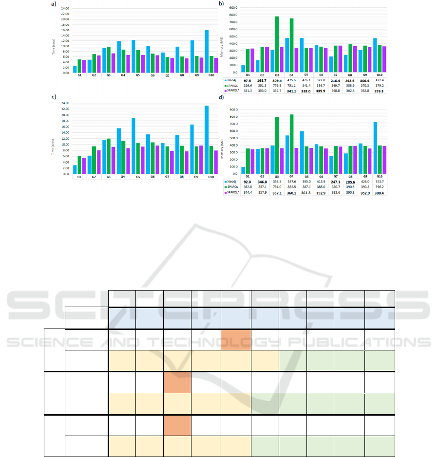
Figure 7: Comparison of Neo4j, SPARQL and SPARQL* for Q2 executions in the graphs G1 to G10. a) Execution time

comparison in seconds for original Q2. b) Maximum main memory consumption usage comparison in MB for original Q2.

c) Execution time comparison in seconds for alternative Q2. d) Maximum main memory consumption comparison in MB for

alternative Q2. In memory charts, for every graph the smallest value is marked in bold.

Table 7: Comparison of Neo4j, SPARQL and SPARQL* for original Q2 executions in the graphs G1 to G10 of the average

time to get a result. We also show the average time of the query in each graph (Figure 7-a). We have marked the groups of

neighbouring graphs with similar behaviour in yellow and green. We have also marked the time relative maximum in orange.

G1 G2 G3 G4 G5 G6 G7 G8 G9 G10

Avg

# Results

13 26 29 33 34 43 40 40 36 41

Neo4j

Avg time

(secs)

2.62 4.86

9.25 11.86

12.21 9.94 7.60 9.76 12.14 16.08

AvgTime/

AvgRes

0.20 0.19 0.31 0.36 0.36 0.23 0.19 0.25 0.34 0.39

SPARQL

Avg time

(secs)

4.99 6.98

9.51 8.60 8.42 7.20 5.82 6.08 6.23 6.21

AvgTime/

AvgRes

0.37 0.27 0.32 0.26 0.25 0.17 0.14 0.15 0.17 0.15

SPARQL*

Avg time

(secs)

4.78 6.40

7.26 6.67 6.70 6.55 5.43 5.37 5.66 5.61

AvgTime/

AvgRes

0.36 0.25 0.25 0.21 0.20 0.15 0.13 0.14 0.16 0.14

This difference between time and memory could

be explained because the nodes and edges between

the Events are charged in memory the first time they

are accessed and remain cached for the rest of the

accesses.

In the case of queries in SPARQL and SPARQL*,

they present memory consumptions with values

similar to those in Q1 and Q2, while the time is much

longer than in any other query.

Before analysing time, it is necessary to comment

that for the experiments, 15 Patients were chosen

between those in the quarter of Patients with more

connected Patients. However, it does not mean that

there must exist connections between all 15 Patients.

What is more, in this work, a bigger graph does not

have to mean more connection between a set of

patients. In Table 8, we can observe that the average

number of results (the number of different paths that

connect a Patient with another) does not increase with

the size of the graphs. In fact, the maximum number

of results is in G7, and the minimum is in G4. The

time series of Neo4j follows the direction of the

number of results: when the number of results

Comparison Between Graph Databases and RDF Engines for Modelling Epidemiological Investigation of Nosocomial Infections

increases, time increases too, and the same when the

number of results decreases.

Curiously, SPARQL* presents a curve more similar

to Neo4j than SPARQL. In fact, the time differences

between SPARQL and SPARQL* stand out in this

query compared to the rest: here, SPARQL presents

times between 115% and 153% bigger than SPARQL*.

This significant difference may be because the majority

of the computation in this query is in traversing edges

with properties, which in SparQL* are represented

with a single edge (actually a statement of a statement),

while SparQL requires one “node of individuals” and

two edges (see Figure 2). Thus, we can judge that the

“edges with properties” from SPARQL* speed up

traversing the graph. Under this assumption, we can

observe that in Q1, where the edges with properties are

barely traversed, the time difference is not so

pronounced, and even in some graphs, SPARQL* is

slower than SPARQL.

4.4 General Aspects

Our experiments suggest that there are common

characteristics between queries related to time and

memory.

First, in Neo4j, there is a strong relation between

time and memory that is perceptible in Q1 and Q2,

but not in Q3. Q1 and Q2 consist of exploring a tree

in which traversing new edges and nodes is the main

computing effort. Contrarily, Q3 works with a limited

set of nodes traversing different combinations of

edges between them. These opposite behaviours give

us a clue about how Neo4j manages memory: as new

edges and nodes are traversed, they are saved in

memory and not deleted until the end of the query (as

long as there is enough memory) to avoid the costly

work of fetching data from disk.

Concerning Neo4j, it is shown that memory usage

does not depend so much on the total size of the graph

but rather on the subgraph to be traversed.

In the case of GraphDB, SPARQL and SPARQL*

present a memory usage similar, but clearly different

from Neo4j. We can observe that in all the

benchmarks, the memory is between 325MB and

400MB (with the exceptions in G3 and G4) and

increases or decreases slightly depending on the

query complexity and the data to save during the

execution (for example, the number of classes of

nodes and edges to return). The size of the graph also

affects the memory usage in GraphDB. We can find

clues about this in Q2 and Q3, where memory

gradually increases from G1 to G10 although the

traversed subgraphs are not necessarily bigger

because they are in a bigger graph.

Figure 8: Comparison of Neo4j, SPARQL and SPARQL*

for Q3 executions in the graphs G1 to G10. a) Execution

time comparison in seconds. b) Maximum main memory

consumption comparison in MB. In memory chart, for

every graph the smallest value is marked in bold.

Table 8: Average number of results of Q3 executions in the

graphs G1 to G10.

Graph Avg #Results

G1 1683

G2 1340

1598

G4 1060

G5 2453

G6 3030

4138

G8 3715

G9 2595

G10 1517

The results strongly suggest Neo4j and GraphDB

work with different memory usage schemes. But to

better understand GraphDB memory usage, it would

be necessary to measure its memory consumption

during query execution and analyse how it changes

from the start to the end. This way, we could confirm

our supposition that memory consumption is stable

throughout the execution and that the maximum

memory is not a peak like in Neo4j.

Regarding time, the results yielded some

interesting findings regarding Neo4j and GraphDB.

While in Neo4j, time changes depending on the type

of query and the size of the subgraph to traverse, in

HEALTHINF 2024 - 17th International Conference on Health Informatics

SPARQL and SPARQL*, time oscillations are lighter.

In Q1 and Q2, they start from a high minimum base

time (around 5 seconds, as opposed to Neo4j’s 2

seconds), but the maximum does not exceed more

than three times the minimum, in contrast to the

maximum times of Neo4j, which can multiply the

minimum by eight.

5 CONCLUSIONS AND FUTURE

WORK

In this research work, we evaluated the performance

of property and knowledge graphs based on triple

stores in the context of spatiotemporal

epidemiological investigation of an infection

outbreak in a hospital. Specifically, we chose Neo4j

as the graph database engine, which has its own data

model and query language, Cypher; and for

knowledge graphs, we used RDF and RDF* as

standard technologies to define the graphs, SPARQL

and SPARQL* languages to query data and GraphDB

database to store the graphs. We defined a domain

model that describes a hospital layout, the

organisation of its healthcare workers and the path of

its patients as a log of all their events. We stated three

queries that are steps of the epidemiological

investigation process and designed a benchmark to

evaluate the queries' time execution and memory in

ten graphs of different sizes whose data come from

the open-data clinical dataset MIMIC-III.

Our experiments provide convincing evidence

that neither in Neo4j nor GraphDB time and memory

are influenced by the total size of the graph, but for

other factors like the complexity of the query (number

of required and optional paths and their length), the

size of the traversed subgraph and if the goal of the

query is retrieving the leaves of a tree or do additional

paths between a set of nodes. Neo4j's performance

highly depends on these factors. For simple queries

and small traversed subgraphs, time and memory can

be half of those of GraphDB. On the other hand, time

and memory on GraphDB present minimum values

much higher than Neo4j but with less aggressive

growth. Thus, SPARQL and SPARQL* will scale

better than Neo4j for queries that need to traverse big

subgraphs.

Our research suggests that the extensions

provided by RDF* with respect to RDF, such as the

addition of the statements about other statements that

allows defining edges with properties, seem

promising for a more complete, compact and

comprehensible modelling. Furthermore, our

experiments suggest that RDF* offers a better

performance of the query execution and less storage

size for the graphs.

It is worth mentioning that RDF and RDF* are

W3C standards and not proprietary formats, as it is

Neo4j. This offers the advantage of greater flexibility

and solidity when choosing between possible

additional tools to work with.

To further compare property graph and knowledge

graph technologies in our context, we plan to define

queries for the rest of the epidemiological

investigation process tasks and, especially, queries to

execute general graph tasks (shortest path,

community detection) over our domain. It would also

be necessary to generate synthetic data that covers the

whole domain model.

ACKNOWLEDGEMENTS

This work was partially funded by the CONFAINCE

project (Ref: PID2021-122194OB-I00), supported

by the Spanish Ministry of Science and

Innovation, the Spanish Agency for Research

(MCIN/AEI/10.13039/501100011033) and, as

appropriate, EFRD A way of making Europe; and by

the GRALENIA project (Ref: 2021/C005/00150055)

supported by the Spanish Ministry of Economic

Affairs and Digital Transformation, the Spanish

Secretariat of State for Digitization and Artificial

Intelligence, Red.es and by the NextGenerationEU

funding. This research was also partially funded by

Fundación Séneca, Región de Murcia (Spain) (Ref:

21460/FPI/20).

REFERENCES

Atemezing, G. A., & Amardeilh, F. (2018). Benchmarking

commercial RDF stores with publications office

dataset. Lecture Notes in Computer Science (Including

Subseries Lecture Notes in Artificial Intelligence and

Lecture Notes in Bioinformatics), 11155 LNCS, 379–

394. https://doi.org/10.1007/978-3-319-98192-5_54

Bellini, P., & Nesi, P. (2018). Performance assessment of

RDF graph databases for smart city services. Journal of

Visual Languages and Computing, 45, 24–38.

https://doi.org/10.1016/J.JVLC.2018.03.002

Ferro, N., & Sinico, L. (2018). Graph Databases

Benchmarking on the Italian Business Register. CEUR

Workshop Proceedings, 2161. https://ceur-ws.org/Vol-

2161/paper43.pdf

Freedman, H., Miller, M. A., Williams, H., & Stoeckert, C.

J. (2020). Scaling and querying a semantically rich,

electronic healthcare graph. CEUR Workshop

Comparison Between Graph Databases and RDF Engines for Modelling Epidemiological Investigation of Nosocomial Infections

Proceedings, 2807. https://ceur-ws.org/Vol-2807/paper

C.pdf

SPARQLWrapper. (2022). https://github.com/RDFLib/

sparqlwrapper

Gu, Z., Yang, X., Jia, W., Xu, C., Yu, P., He, X., Chen, H.,

& Lin, Y. (2022). StrokePEO: Construction of a

Clinical Ontology for Physical Examination of Stroke.

Proceedings - 2022 9th International Conference on

Digital Home, ICDH 2022, 218–223.

https://doi.org/10.1109/ICDH57206.2022.00041

Hohenstein, U., & Jergler, M. (2019). Database

performance comparisons: An inspection of fairness.

DATA 2019 - Proceedings of the 8th International

Conference on Data Science, Technology and

Applications, 243–250. https://doi.org/10.5220/00079

26602430250

Johnson, A. E. W., Pollard, T. J., Shen, L., Lehman, L. H.,

Feng, M., Ghassemi, M., Moody, B., Szolovits, P.,

Anthony Celi, L., & Mark, R. G. (2016). MIMIC-III, a

freely accessible critical care database. Scientific Data,

3(1), 160035. https://doi.org/10.1038/sdata.2016.35

Kiourtis, A., Mavrogiorgou, A., Menychtas, A.,

Maglogiannis, I., & Kyriazis, D. (2019). Structurally

Mapping Healthcare Data to HL7 FHIR through

Ontology Alignment. Journal of Medical Systems,

43(3). https://doi.org/10.1007/S10916-019-1183-Y

Kovács, T., Simon, G., & Mezei, G. (2019). Benchmarking

graph database backends - What works well with

wikidata? Acta Cybernetica, 24(1), 43–60.

https://doi.org/10.14232/ACTACYB.24.1.2019.5

Leavitt, N. (2010). Will NoSQL Databases Live Up to Their

Promise? Computer, 43(2), 12–14. https://doi.org/10.11

09/MC.2010.58

Li, W., Wang, S., Wu, S., Gu, Z., & Tian, Y. (2022).

Performance benchmark on semantic web repositories

for spatially explicit knowledge graph applications.

Computers, Environment and Urban Systems, 98.

https://doi.org/10.1016/J.COMPENVURBSYS.2022.1

01884

LIU, D., WEI, C., XIA, S., & YAN, J. (2022). Construction

and application of knowledge graph of Treatise on

Febrile Diseases. Digital Chinese Medicine, 5(4), 394–

405. https://doi.org/10.1016/J.DCMED.2022.12.006

Monteiro, J., Sá, F., & Bernardino, J. (2023). Experimental

Evaluation of Graph Databases: JanusGraph, Nebula

Graph, Neo4j, and TigerGraph. Applied Sciences

(Switzerland), 13(9). https://doi.org/10.3390/APP1309

5770

Pujante-Otalora, L., Canovas-Segura, B., Campos, M., &

Juarez, J. M. (2023). The use of networks in spatial and

temporal computational models for outbreak spread in

epidemiology: A systematic review. Journal of

Biomedical Informatics, 143, 104422. https://doi.org/

10.1016/J.JBI.2023.104422

RDF 1.1 Concepts and Abstract Syntax. (n.d.). Retrieved

September 26, 2023, from https://www.w3.org/TR/rdf

11-concepts/

RDF-star and SPARQL-star. (n.d.). Retrieved September

25, 2023, from https://www.w3.org/2021/12/rdf-

star.html

Rivas, A., & Vidal, M. E. (2021). Capturing Knowledge

about Drug-Drug Interactions to Enhance Treatment

Effectiveness. K-CAP 2021 - Proceedings of the 11th

Knowledge Capture Conference, 33–40.

https://doi.org/10.1145/3460210.3493560

SPARQL 1.1 Query Language. (n.d.). Retrieved September

26, 2023, from https://www.w3.org/TR/sparql11-

query/

Trevena, W., Lal, A., Zec, S., Cubro, E., Zhong, X., Dong,

Y., & Gajic, O. (2022). Modeling of Critically Ill Patient

Pathways to Support Intensive Care Delivery. IEEE

Robotics and Automation Letters, 7(3), 7287–7294.

https://doi.org/10.1109/LRA.2022.3183253

Neo4j Python driver. (2023). https://neo4j.com/docs/

getting-started/languages-guides/neo4j-python/

Wang, R., Yang, Z., Zhang, W., & Lin, X. (2020). An

empirical study on recent graph database systems.

Lecture Notes in Computer Science (Including

Subseries Lecture Notes in Artificial Intelligence and

Lecture Notes in Bioinformatics), 12274 LNAI, 328–

340. https://doi.org/10.1007/978-3-030-55130-8_29

Yin, Y., Li, G. Z., Wang, Y., Zhang, Q., Wang, M., & Zhang,

L. (2021). Study on construction and application of

knowledge graph of TCM diagnosis and treatment of

viral hepatitis B. Proceedings - 2021 IEEE International

Conference on Bioinformatics and Biomedicine, BIBM

2021, 3906–3911. https://doi.org/10.1109/BIBM526

15.2021.9669760

HEALTHINF 2024 - 17th International Conference on Health Informatics