Outlier Detection in MET Data Using Subspace Outlier Detection
Method
Dupuy Rony Charles
1,2 a
, Pascal Pultrini
2
and Andrea Tettamanzi
1 b
1
Universit
´
e C
ˆ
ote d’Azur, I3S, Inria, Sophia Antipolis, France
2
Doriane Research Softare & Consulting, Av. Jean Medecin, Nice, France
Keywords:
Outlier Detection, Multi-Environment Field Trials, Genomic Prediction, Machine Learning Clustering
Methods.
Abstract:
In plant breeding, Multi-Environment Field Trials (MET) are commonly used to evaluate genotypes for mul-
tiple traits and to estimate their genetic breeding value using Genomic Prediction (GP). The occurrence of
outliers in MET is common and is known to have a negative impact on the accuracy of the GP. Therefore,
identification of outliers in MET prior to GP analysis can lead to better results. However, Outlier Detection
(OD) in MET is often overlooked. Indeed, MET give rise to different level of residuals which favor the pres-
ence of swamping and masking effects where ideal sample points may be portrayed as outliers instead of the
true ones. Consequently, without a sensitive and robust outlier detection algorithm, OD can be a waste of time
and potentially degrade the accuracy prediction of the GP, especially when the data set is not huge. In this
study, we compared various robust outlier methods from different approaches to determine which one is most
suitable for identifying MET anomalies. Each method has been tested on eleven real-world MET data sets.
Results are validated by injecting a proportion of artificial outliers in each set. The Subspace Outlier Detection
Method stands out as the most promising among the tested methods.
1 INTRODUCTION
In plant breeding, multi-environment field trials
(MET) are considered as the source of phenotypes.
Essentially, they are used to evaluate plants for multi-
ple target traits in various environments and to pre-
dict their estimated genetic values (GEBVs) (Lee
et al., 2023). The latter are commonly calculated
through genomic prediction (GP) analysis. GP com-
putes GEBV by using genetic markers information as
well as phenotypes in statistical learning methods de-
velopment (Meuwissen et al., 2001).
MET are experiments involving many genotypes,
conducted at multiple sites over multiple years.
Whenever multiple measurements are obtained, there
is always a chance of getting outliers, and MET are
no exception. In MET, anomalies can arise from dis-
tant observations, geographic location, year, or sim-
ply subjectivity in the measurement process. The var-
ious origins of anomalies may increase the difficulty
of distinguishing them from benign data.
a
https://orcid.org/0009-0006-4879-9933
b
https://orcid.org/0000-0002-8877-4654
A common need when analyzing real-world
datasets is to determine which instances stand out
as being dissimilar to all others. Such instances are
known as anomalies or outliers. Hawkins described
them as observations that deviate from other obser-
vations so significantly as to arouse the suspicions
that they were generated by a different mechanisms
(Hawkins, 1980). Outlier detection becomes an im-
portant pre-processing step to identify such dubious
instances (Yao et al., 2020). Performing that step prior
to GP analysis becomes even more important because
it gets rid of data points that can negatively impact the
accuracy of the model prediction (Estaghvirou et al.,
2014).
The literature on outlier analysis is enormous.
A large number of authors have proposed different
methods, books, survey and review articles on the
subject. For instance, (Hawkins, 1980), (Barnett
et al., 1994), (Aggarwal and Aggarwal, 2017), and
(Rousseeuw and Leroy, 2005) are classic books deal-
ing with outlier analysis.
Beckman and Cook (Beckman and Cook, 1983)
have reviewed rejection techniques for multiple out-
liers as the effects of masking and swamping, as well
Charles, D., Pultrini, P. and Tettamanzi, A.
Outlier Detection in MET Data Using Subspace Outlier Detection Method.
DOI: 10.5220/0012318000003636
Paper published under CC license (CC BY-NC-ND 4.0)
In Proceedings of the 16th International Conference on Agents and Artificial Intelligence (ICAART 2024) - Volume 3, pages 243-250
ISBN: 978-989-758-680-4; ISSN: 2184-433X
Proceedings Copyright © 2024 by SCITEPRESS – Science and Technology Publications, Lda.
243

as works on outliers in circular data, discriminant
analysis, experimental design, multivariate data, gen-
eralized linear models, distributions other than nor-
mal, time series, etc. (Markou and Singh, 2003) have
provided a state-of-the-art review in the area of nov-
elty detection based on statistical approaches. (Sajesh
and Srinivasan, 2012) presented a review of mul-
tivariate outlier detection methods especially robust
distance based methods. They have also proposed
a computationally efficient outlier detection method
using the comedian approach with high breakdown
value and low computation time. And more recently,
(Samariya and Thakkar, 2021) have listed different
types of outlier detection algorithm and their domains
of applications as well as some evaluation measures.
Indeed, several outlier detection algorithms have
been applied on MET data, such as the Cook’s dis-
tance, model statistics based on confidence ellipsoid
(Cook, 1977), and (Christensen et al., 1992), the lo-
cally centered Mahalanobis distance, which centers
the covariance matrix at each that sample (Todes-
chini et al., 2013), etc. However, to the best of our
knowledge, no comparisons have been made between
different outlier detection methods, and no genuine
outlier detection method has ever been strongly rec-
ommended for identifying anomalies in MET data.
The latter can be very complex and challenging to be
cleaned (DeLacy et al., 1996).
To bridge this gap, in this study, the focus is to
provide a critical comparison, on this specific task,
of various multivariate outlier detection algorithms
from different approaches such as hierarchical clus-
tering or connectivity e.g: Mahalanobis Distance,
Mean Shift Outlier Model), influential (e.g: Cook’s
Distance), distribution (e.g: One-Class Support Vec-
tor Machine), centroid (e.g: K-Means Clustering), en-
semble (e.g: Isolation Forest), density (e.g: Density-
Based Spatial Clustering of Applications with Noise),
probabilistic (e.g: Gaussian Mixture Model), sub-
space (e.g: Subspace Outlier Detection Algorithm,
Auto-Encoders for Outlier Detection) to determine
which ones are best suited to identify outliers (espe-
cially mild ones) in MET samples. To conduct that
comparison, while taking into account the aggressive-
ness and robustness of each method, we consider two
scenarios: first, compute the GP without identifying
the anomalies, and then recompute it with anoma-
lies identified and removed. Second, inject artificial
anomalies into the samples and use the same methods
to retrieve them. All scenarios and methods have been
run on each of the eleven different MET data sets. The
method with the best score in both scenarios will be
considered as the most appropriate one.
The rest of this paper is organized as follows. Sec-
tion 2-materials and methods, where we present the
data sets we have worked with, summarize the differ-
ent outlier detection algorithms considered, define the
genomic prediction method and comparison metrics
used, as well as the validation methodologies. In Sec-
tion 3, we present and discuss the results. In Section 4
we draw some conclusions.
2 MATERIALS AND METHODS
2.1 Data Summary
For this study of multivariate anomalies within MET,
we inherited a few historical datasets from three dif-
ferent sources:
• RAGT - A European seed company for field
crops and livestock soft winter wheat, durum
wheat, grain maize, rapeseed, sunflower, soy-
beans, sorghum and maize.
1
Those MET have
been separately conducted in three countries
(France, Hungary and Ukraine), within up to
thirty-one (31) locations, on hybrid grain maize
from 2014 to 2021. MET data is the result of a
manual annotation process carried out by the com-
pany’s experts.
• 2016 CAIGE - 2016 CIMMYT Austrialia
ICARDA Germplasm Evaluation (CAIGE).
2
Those datasets relate to bread wheat trials. The
latter were conducted at eight locations in Aus-
tralia, where 240 varieties have been tested on
seven trials. Each experience employed a partially
replicated design with two blocks and p ranging
from 0.23 to 0.39.
We have built up a bank of eleven real-world MET
datasets from the two sources presented above. Each
sample is a combination of phenotypes and genotypes
(single nucleotide polymorphisms genetic markers).
The samples vary in size. They are varieties of maize
and bread wheat.
The code and data from this study are available in
a public repository.
3
2.2 Outlier Detection Methods
Below is a list of outlier detection algorithms from
different approaches that can be used to identify
1
https://ragt-semences.fr/fr-fr Accessed on June 12,
2023.
2
https://www.caigeproject.org.au/
icarda-data-2016shipment Accessed on June 12, 2023.
3
https://github.com/charlesdupuyrony/
outlierDetectionComparison
ICAART 2024 - 16th International Conference on Agents and Artificial Intelligence
244

doubtful cases in a multivariate dataset as complex
as the MET. In this study, they have been imple-
mented and optimized to fit the data distributions de-
fined above.
• Mahalanobis Distance (d
M
) - A measure of the
distance between an observation
−→
x
i
and a dis-
tribution D. An observation with a large d
M
is more likely an outlier. The d
M
of
−→
x
i
=
(x
i1
,x
i2
,x
i3
,...,x
in
)
T
∈ D on R
n
is obtained via the
equation:
d
M
(
−→
x
i
,D) =
q
(
−→
x
i
−
−→
µ )
T
S
−1
(
−→
x
i
−
−→
µ ), (1)
where
−→
µ = (µ
1
,µ
2
,µ
3
,...,µ
n
)
T
is the vector of
features means and S is the covariance matrix.
Mahalanobis distance approach is based on the as-
sumption that normal data belong to a cluster in
the dataset, while outliers either do not belong to
any cluster. Therefore, elements from the same
cluster are quite similar and are closer to each
other than the rest.
• Cook’s Distance (D) - A commonly used esti-
mate of the influence of a data point in a least-
squares regression analysis. Instances with large
influence may be outliers. The Cook distance of
an observation i, denoted by D
i
, is defined as the
sum of all the changes in the regression model
when observation i is removed from it:
D
i
=
∑
n
j=1
( ˆy
j
− ˆy
j(i)
)
2
ps
2
, (2)
where ˆy
j(i)
is the fitted response value obtained
when excluding observation i, p is the number of
fitted parameters, s
2
is the mean squared error of
the regression model, and ˆy
j
is the fitted response
value obtained with observation i.
• Mean Shift Outlier Model (MSOM) - The
mean-shift technique replaces every object by the
mean of its k-nearest neighbors, which essentially
removes the effect of outliers before clustering,
without the need for knowing the outliers. The ex-
plicit formulation of the mean shift for point υ
(i)
is
υ
(i)
=
∑
N
j=1
x
j
g((υ
(i−1)
− x
j
)
T
H
−2
(υ
(i−1)
− x
j
))
∑
N
j=1
g((υ
(i−1)
− x
j
)
T
H
−2
(υ
(i−1)
− x
j
))
,
(3)
where the support is defined by the points in x
i
∈
1,2,...,N and the kernel bandwidth parameter is
identified as H. H is assumed to be of full rank
and symmetric in this formula.
This algorithm identifies local maxima by updat-
ing υ(i) at each iteration, starting with a set of ini-
tial points. Iteration continues until a fixed num-
ber of iterations is met or
∥υ
(i)
− υ
(i−1)
∥
∥υ
(i−1)
∥
< δ, (4)
where δ is an acceptable tolerance. Outliers are
identified based on the distance shifted.
• One Class Support Vector Machines (OC-
SVM) - Unsupervised learning technique derived
from support vector machines, in which all train-
ing data belong to the first class. OC-SVM con-
structs a decision function based on a hyper-
sphere to best separate one class sample from the
others with the largest margin possible. The math-
ematical expression to compute a hyper-sphere
with centre c and radius r is
∥φ(x
i
) − c∥
2
≤ r
2
, (5)
where φ(x
i
) is the hyper-sphere transformation of
instance i. With the presence of outliers within
the dataset, minimizing the hyper-sphere radius is
equivalent to
min
r,c,ξ
r
2
+
1
υn
n
∑
i=1
ξ
i
(6)
subject to
∥φ(x
i
) − c∥
2
≤ r
2
+ ξ
i
, (7)
where i = 1,2,...,n, n being the number of rows
in the dataset.
• K-Means Clustering Algorithm (K-Means) - A
method of vector quantization that aims to par-
tition n observations into k clusters in which an
observation belongs to the cluster with the near-
est mean (cluster centroid) serving as the proto-
type of the cluster. Assuming X a distribution of
n observations where X = {X
1
,X
2
,...,X
n
} and X
i
the feature i. The goal of K-Means is to find a
dataset Z = {Z
1
,Z
2
,...Z
m
,...,Z
k
} (with 2 ≤ k ≤ n)
is to minimize the sum of inter-cluster dispersion
as shown in the following equation
J
c
=
k
∑
m=1
n
∑
i=1
d(X
i
,Z
m
), (8)
where Z
m
is the m
th
clustering center and
d(X
i
,Z
m
) is the distance between observation i
and the m
th
cluster center. If the function J
c
is
minimized, then i has been allocated to the most
suitable cluster. Therefore, the distance J
i
be-
comes
J
i
= d(X
i
,Z
m
) = X
i
−Z
m
= min
m=1,2,...,k
X
i
−X
m
. (9)
Outlier Detection in MET Data Using Subspace Outlier Detection Method
245

• Isolation Forest Method (iForest) - An approach
that employs binary trees to detect anomalies. Let
X = X = {x
1
,x
2
,...,x
d
} be a set of d-dimensional
distributions and X
′
= {x
i
,x
k
,...,x
l
} where i, k
and l ∈ {1,2,...,d}. A sample of φ instances
X
′
∈ X is used to build an isolation tree. Re-
cursively, X divided by randomly selecting an at-
tribute q and a split value p, until either (i) the
node has only one instance or (ii) all data at the
node have the same values.
Assuming all instances are distinct, each instance
is isolated to an external node when an iTree is
fully grown, in which case the number of external
nodes is ψ and the number of internal nodes is ψ−
1; the total number of nodes of an iTree is 2ψ −
1; the memory requirement is thus bounded and
only grows linearly with ψ. While the maximum
possible height of the iTree grows in the order of
φ, the average height grows in the order of logψ.
• Density-Based Spatial Clustering of Applica-
tions with Noise (DBSCAN) - A density-based
clustering algorithm that uses two parameters: ep-
silon and minimum of points to determine a clus-
ter. Epsilon represents the maximum distance
from a data point i to evaluate if other points be-
long to the same cluster membership. Minimum
of points is the minimum number of points re-
quired inside that hyper-sphere around data point i
to be classified as a core point. Any point j whese
distance from i is greater than epsilon cannot be in
the same hyper-sphere. At the end, each point will
fall into one of the three categories: core point,
border point, or noise point. An outlier has fewer
than the minimum of points surrounding it, and is
reachable from no core points.
• Gaussian Mixture Model (GMM) - A paramet-
ric probability model that assumes all the data
points are generated from a mixture of a finite
number (M) of Gaussian distributions with un-
known parameters. GMM is a weighted sum of
M component Gaussian densities as given by the
following equation
p(X/λ) =
M
∑
i=1
w
i
g(X|µ
i
,
∑
i
), (10)
where X is a D-dimensional continuous-valued
data vector (i.e., the sample studied, and D is
the number of features), w
i
with i = 1,2,...,M
are the mixture weights, and g(X|µ
i
,
∑
i
) for i =
1,2,...,M are the components Gaussian densi-
ties.
Each component density is D-variate Gaussian
function of the form
g(X|µ
i
,
∑
i
) =
1
p
(2π)
D
|
∑
i
|
exp
−
1
2
(X−µ
i
)
′
∑
−1
i
(X−µ
i
)
,
(11)
with mean vector µ
i
and covariance matrix
∑
i
.
The mixture weights satisfy the constraint that
∑
M
i=1
= 1. To detect anomalies using a GMM,
we compute the sum of the probability density
function of each sample X
i
= [X
1
i
,X
2
i
,...,X
D
i
] for
each of the two clusters S
p
and S
q
, respectively
the cluster of normal sample and the cluster of
anomalies. Assuming the bigger cluster S
p
con-
tains normal data sample, a density profile is con-
structed with S being the ratio S
q
/S
p
.
• Subspace Outlier Detection Algorithm (SOD) -
An outlier detection model based on the assump-
tions that outliers are lost in low dimensional sub-
spaces, when full-dimensional analysis is used.
Such an approach filters out the additive noise ef-
fects of the large number of dimensions and re-
sults in more robust outliers.
A subspace model is built upfront and each data
point is scored with respect to that model. Points
are typically scored by using an ensemble score
of the results obtained from different models. A
threshold is defined to determine the outlying
points from the normal ones.
• Auto Encoders for Anomaly Detection (AEAD)
- An unsupervised version of neural network that
is used for data encoding. We have implemented
an auto encoder with three layers. The input layer
contains a number n of neurons, which corre-
sponds to the number of dimensions in the sam-
ple. The number of neurons in the hidden layer
is set to a fraction of the number of dimensions
in the data set being examined. The ReLU ac-
tivation is used as the activation function for the
output layer. The goal is to learn the weights that
minimize the reconstruction error defined by the
following equation:
R
e,d
= ||X −d(e(X))||
2
, (12)
where e and d are, respectively, the encoder and
decoder functions y = e(X) and
ˆ
X = d(y). Learn-
ing the weights of the model is done via the
AdaDelta gradient optimizer in a number n
e
of
training epochs.
2.3 Linear Mixed Model
The most popular statistical learning methods used in
GP are the linear mixed models (LMM) (also known
as random effects models) (Montesinos L
´
opez et al.,
ICAART 2024 - 16th International Conference on Agents and Artificial Intelligence
246

2022). However, the family of random effects mod-
els is known to be sensitive to the presence of out-
liers resulting in lower accuracy of genetic breeding
value predictions (Estaghvirou et al., 2014). The ma-
trix form of a linear mixed model can be defined as
Y = Xβ + Zu + ε, (13)
where Y is the vector of response variables, X is the
design matrix of fixed effects, β is the vector of fixed
effects, Z is the design matrix of random effects, u
is the vector of random effects distributed as N(0,
∑
),
where
∑
is a variance-covariance matrix of random
effects, and ε is a vector of residuals distributed as
N(0,R), where R is a variance-covariance matrix of
residual effects. GEBV is the solution
ˆ
u of that mixed
model equation. A form of Ridge regression, and
its predictions called ridge-regression best linear un-
biased predictions (RR-BLUPs) has been recognized
as a popular, simple and accurate method for obtain-
ing genetic breeding values (Montesinos L
´
opez et al.,
2022).
2.4 Evaluation Measures
Each scenario has its own metrics. In the first
scenario, we consider the root mean squared error
(RMSE) to evaluate the effectiveness of the methods
and the correlation coefficient (CC) to measure the
strength of the linear relationship between the actual
value (y) and the predicted value( ˆy). The method with
smallest RMSE and the greatest CC is the most ap-
propriate one.
Since the methods run on 11 samples, a method
may be effective on one sample and less effective on
another. To take account of their performance on all
samples, we assign a score to the three most effec-
tive methods for RMSE and CC. The most effective
method for a measurement on one sample receives 3
points, the second 2, the third 1, the others 0 points. In
sum, for each sample, a method can have a maximum
score of 6. Eventually, the method with the highest
total score is taken to be the most appropriate one.
In the second scenario, we consider the Area Un-
der the Curve (AUC) of the Receiver Operating Char-
acteristic (ROC) to evaluate how much a method is
capable of distinguishing between normal and abnor-
mal data points, especially the injected ones.
In addition, we also calculate the time needed for
each method to identify anomalies. Although execu-
tion time has no effect on model accuracy, it can be
a determining factor when choosing a model in prac-
tice.
2.5 Experience Computational
Procedure
Scenario-I To compare the methods listed above,
two scenarios are worth considering for each of the
MET samples. On one hand, we train linear mixed
models (using the rrBLUP algorithm) with these data
and the genetic markers. Then, we use these models
to predict the genetic selection value of a trait with
very low heritability: the yield for instance. In this
case, we assume the presence of outliers in the data
sets, without knowing their position. However, if they
do exist, we assume that their presence will have a
negative impact on the accuracy of the linear mixed
model prediction. In other words, if an outlier detec-
tion method is aggressive enough to identify genuine
outliers, we can expect the model’s prediction accu-
racy to be higher than when those instances were still
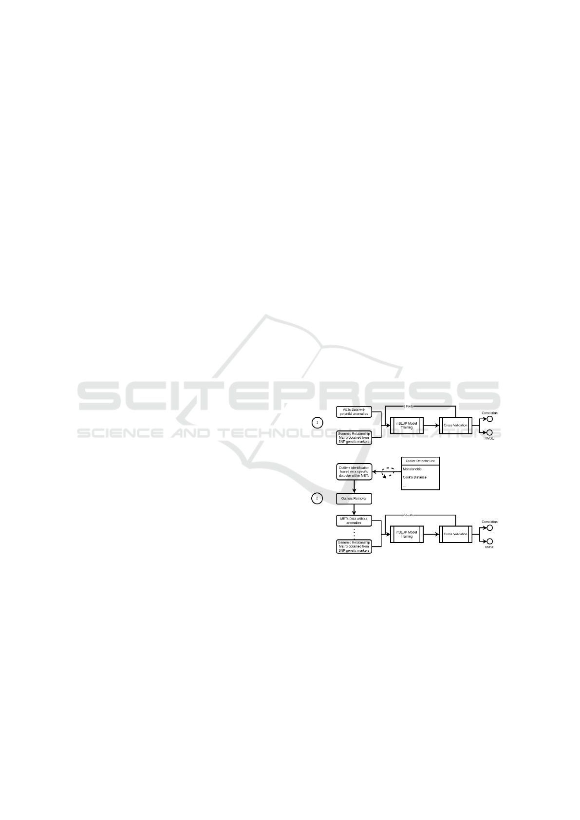
in that dataset. As shown in Figure 1, this approach
has two phases: In Phase 1, we establish a reference
accuracy and correlation by training a model based
on METs and genetic markers, without seeking to re-
move anomalies. The accuracy and correlation co-
efficient obtained after predicting the genetic breed-
ing value are referred to as reference values, as they
will be used to compare the effectiveness of the detec-
tor. In the second phase, the method determines the
Figure 1: scenario 1 - Using linear mixed model to evaluate
outlier detection methods.
anomalies present within the MET. Those instances
are removed from the sample, then we train the LMM
with the remaining phenotypes and the correspond-
ing genetic markers. That trained model is also use to
compute the accuracy of the prediction and the corre-
lation coefficient. The values obtained are later com-
pare to the reference values to assess the effectiveness
of the detection method used.
Obviously, identifying the outliers within a sam-
ple adds additional time to the process, and that time
Outlier Detection in MET Data Using Subspace Outlier Detection Method
247

varies depending on the detection method used. So,
in the Phase 2, we also compute the time consumed
by the detection method. That process is repeated for
all the 10 methods on all the 11 samples.
Scenario-II This second approach involves inject-
ing artificial anomalies into the MET datasets, then
using the same anomaly detection methods listed
above to detect them. This way, we can compare the
methods by computing the rates of true and false pos-
itives as well as the area under the curve of the re-
ceiver’s operating characteristic.
An amount of artificial outliers equivalent to 10%
of the dataset was generated and injected into the
dataset. Then, we use the synthetic minority oversam-
pling technique (SMOTE), which is an oversampling
technique that generates synthetic samples from mi-
nority class in our case, the artificial anomalies. The
same process has been implemented for all the sam-
ples.
2.6 Validation Methodology
In Scenario-I, the difference between the predicted
breeding values and the observed phenotypic values
(respectively ˆy and y), called predictive ability, de-
noted by r
ˆy
, is estimated for all the listed methods
using a 5-fold cross validation.
In Scenario-II, the 5-fold cross validation is no
longer optimal. We use a different member of the
k-fold validation methods family known as stratified
k-fold cross validation. That latter still partitions the
dataset into k (k = 5) folds, except that each fold has
an equal number of instances of injected outliers as
well as normal observations.
3 RESULTS
Scenario-I shows that all the outlier detectors find
some outliers in all the samples. Each method finds
different anomalies for the same dataset. Further-
more, rrBLUP has better accuracy prediction when
most the MET are cleaned by most of the outlier de-
tection methods.
The authentic method is not an outlier analysis
method. It corresponds to Phase 1 of Scenario-I,
which involves training the models using MET data,
without applying a method for identifying and remov-
ing outliers. As shown in Table-1 and Table-2, there
is no single method that allows to consistently have
the smallest error while having the largest correlation
on all the samples. However, the Gaussian Mixture
Model and the Subspace Outlier Detection Algorithm
appear to be the two most appropriate methods. The
latter takes longer to identify its outliers.
Table 1: Scenario-I - Top 3 outlier detection methods based on the samples.
Dataset RMSE-3 RMSE-2 RMSE-1 CC-3 CC-2 CC-1
D-0312 Gaussian Subspace OC-SVM Subspace iForest OC-SVM
D-0482 Gaussian Cook AEncoder Mahalanobis Cook AEncoder
D-0518 Subspace OC-SVM Cook K-Means Gaussian OC-SVM
D-0526 Mahalanobis DBSCAN Subspace Subspace DBSCAN AEncoder
D-0668 Gaussian Mahalanobis iForest Mahalanobis Cook AEncoder
D-0750 Gaussian Mahalanobis OC-SVM Subspace AEncoder iForest
D-0919 K-Means Mahalanobis iForest K-Means AEncoder MS-Outlier
D-1694 Cook Mahalanobis AEncoder MS-Outlier Subspace AEncoder
D-2879 DBSCAN K-Means OC-SVM Subspace Gaussian K-Means
D-5979 MS-Outlier Gaussian Cook Subspace Gaussian MS-Outlier
D-6770 Gaussian OC-SVM Mahalanobis Gaussian Subspace iForest
Table 2: Scenario-I - Weights of the top 3 outlier detection methods based on the samples.
Dataset Gaus. Subs. OC-SVM Maha. K-Means A.Enc iFo. MS-Out. Cook DBSCAN
1 D-0312 3 5 2 0 0 0 2 0 0 0
2 D-0482 3 0 0 3 0 2 0 0 4 0
3 D-0518 2 3 3 0 3 0 0 0 1 0
4 D-0526 0 4 0 3 0 1 0 0 0 4
5 D-0668 3 0 0 5 0 1 1 0 2 0
6 D-0750 3 3 1 2 0 2 1 0 0 0
7 D-0919 0 0 0 2 6 2 1 1 0 0
8 D-1694 0 2 0 2 0 2 0 3 3 0
9 D-2879 2 3 1 0 3 0 0 0 0 3
10 D-5979 4 3 0 0 0 0 0 4 1 0
11 D-6770 6 2 2 1 0 0 1 0 0 0
Total 26 25 9 18 12 10 10 8 11 7
ICAART 2024 - 16th International Conference on Agents and Artificial Intelligence
248

Table 3: Scenario-II - AUC score obtained by anomaly detection methods on each sample.
Dataset Gaussian Subspace OC-SVM Mahala. K-Means A. Enc. iForest MS-Out. Cook DBSCAN
D-0312 0.435943 0.903800 0.480657 0.511021 0.487544 0.586328 0.502009 0.459649 0.690104 0.902135
D-0482 0.473502 0.922811 0.544211 0.485167 0.571573 0.490975 0.509505 0.500048 0.684092 0.746544
D-0518 0.453863 0.942060 0.517993 0.469833 0.487124 0.454894 0.498845 0.489394 0.709310 0.744635
D-0526 0.400634 0.912342 0.595078 0.632893 0.536120 0.517412 0.540668 0.509514 0.752603 0.922833
D-0668 0.831115 0.903544 0.588596 0.541274 0.469429 0.518911 0.599436 0.505364 0.703132 0.860233
D-0750 0.501481 0.942222 0.511111 0.505926 0.443704 0.511111 0.564444 0.484444 0.695556 0.871111
D-0919 0.442563 0.974002 0.611673 0.604450 0.554157 0.528929 0.629797 0.446460 0.721617 0.971584
D-1694 0.677552 0.967541 0.555002 0.524090 0.486573 0.520178 0.535245 0.492919 0.745898 0.866230
D-2879 0.622051 0.958703 0.587756 0.551876 0.487369 0.515799 0.569440 0.467643 0.756172 0.867426
D-5979 0.610430 0.983646 0.598377 0.532047 0.524492 0.509467 0.618635 0.476551 0.697508 0.955492
D-6770 0.634499 0.979403 0.560397 0.496800 0.490727 0.565075 0.571229 0.533317 0.734778 0.935089
The results of Scenario-I confirm the hypothesis
according to which it is highly probable to have out-
liers in the MET. Some of them have lots of dubi-
ous instances. Some outlier detectors may have found
about forty-five percent outliers in some samples (e.g:
DBSCAN on D-0518). However, we are not sure
whether those identified data points are real anoma-
lies or the detection methods were very aggressive fil-
tering out too many benign instances.
Table-3 shows the AUC score for each anomaly
detection method on each of the data samples for
Scenario-II. Again, the subspace outlier detection al-
gorithm clearly stood out from the others by having
the best score on almost all samples. SOD has re-
trieved the injected outliers with high degree of preci-
sion.
In summary, based on those scenarios, the Sub-
space Outlier Detection Algorithm seems the most ap-
propriate to identify dubious instances into multivari-
ate MET data.
4 CONCLUSIONS
We compared various outlier detection techniques
from different approaches by testing them on eleven
real TEM data from corn and soft wheat. Use two dif-
ferent approaches. The first approach simulates what
can happen in reality when no prior knowledge about
the nature of the sampling points is available. In such
a case, the precision analysis prediction can be a good
indication. Knowing that, for the same learning al-
gorithm, better precision can indicate that the inputs
are better. Unlike the first scenario, in the second the
outlier data points are well known and thus the per-
formance of the outlier detectors could be measured
effectively.
The subspace outlier detection method stands out
in its performance compared to other optimized and
tested methods considered for this study, in both ap-
proaches. Thus, it is best suited to identify outliers in
MET data.
MET data collected based on the annotation pro-
cess (especially manual annotation), can be very sub-
jective and can therefore be easily transformed into
high-dimensional datasets. Such ease could explain
the results observed when using the subspace out-
lier detection method which is a promising approach
for finding outlier instances by projecting the samples
into lower dimensional spaces. That method is able
able to detect outliers which are undetectable in the
full space due to irrelevant attributes interference.
Despite the excellent results observed with the
subspace outlier detection method, it would be nec-
essary to study it on other MET data generated from
other species and, above all, annotated differently, be-
fore attesting that it is the most powerful and robust
outlier detection methods for any MET Data.
REFERENCES
Aggarwal, C. C. and Aggarwal, C. C. (2017). An introduc-
tion to outlier analysis. Springer.
Barnett, V., Lewis, T., et al. (1994). Outliers in statistical
data, volume 3. Wiley New York.
Beckman, R. J. and Cook, R. D. (1983). Outliers. Techno-
metrics, 25(2):119–149.
Christensen, R., Pearson, L. M., and Johnson, W. (1992).
Case-deletion diagnostics for mixed models. Techno-
metrics, 34(1):38–45.
Cook, R. (1977). Detection of influential observations in
linear regression, in “technometric”, 19. I5-18.
DeLacy, I., Basford, K., Cooper, M., Bull, J., McLaren, C.,
et al. (1996). Analysis of multi-environment trials–
an historical perspective. Plant adaptation and crop
improvement, 39124:39–124.
Estaghvirou, S. B. O., Ogutu, J. O., and Piepho, H.-P.
(2014). Influence of outliers on accuracy estimation
in genomic prediction in plant breeding. G3: Genes,
Genomes, Genetics, 4(12):2317–2328.
Hawkins, D. M. (1980). Identification of outliers, vol-
ume 11. Springer.
Lee, S. Y., Lee, H.-S., Lee, C.-M., Ha, S.-K., Park, H.-
M., Lee, S.-M., Kwon, Y., Jeung, J.-U., and Mo, Y.
Outlier Detection in MET Data Using Subspace Outlier Detection Method
249

(2023). Multi-environment trials and stability analy-
sis for yield-related traits of commercial rice cultivars.
Agriculture, 13(2):256.
Markou, M. and Singh, S. (2003). Novelty detection: a re-
view—part 1: statistical approaches. Signal process-
ing, 83(12):2481–2497.
Meuwissen, T. H., Hayes, B. J., and Goddard, M. (2001).
Prediction of total genetic value using genome-wide
dense marker maps. genetics, 157(4):1819–1829.
Montesinos L
´
opez, O. A., Montesinos L
´
opez, A., and
Crossa, J. (2022). Multivariate statistical machine
learning methods for genomic prediction. Springer
Nature.
Rousseeuw, P. J. and Leroy, A. M. (2005). Robust regres-
sion and outlier detection. John wiley & sons.
Sajesh, T. and Srinivasan, M. (2012). Outlier detection for
high dimensional data using the comedian approach.
Journal of Statistical Computation and Simulation,
82(5):745–757.
Samariya, D. and Thakkar, A. (2021). A comprehensive
survey of anomaly detection algorithms. Annals of
Data Science, pages 1–22.
Todeschini, R., Ballabio, D., Consonni, V., Sahigara, F., and
Filzmoser, P. (2013). Locally centred mahalanobis
distance: a new distance measure with salient features
towards outlier detection. Analytica chimica acta,
787:1–9.
Yao, Y., Wang, X., Xu, M., Pu, Z., Atkins, E., and Crandall,
D. (2020). When, where, and what? a new dataset for
anomaly detection in driving videos. arXiv preprint
arXiv:2004.03044.
ICAART 2024 - 16th International Conference on Agents and Artificial Intelligence
250