Botnet Detection by Integrating Multiple Machine Learning Models
Thanawat Tejapijaya
1 a
, Prarinya Siritanawan
2,∗ b
, Karin Sumongkayothin
1,∗ c
and
Kazunori Kotani
2 d
1
Mahidol University, Nakhon Pathom, Thailand
2
Japan Advanced Institute of Science and Technology, Nomi, Ishikawa, Japan
Keywords:
Botnet Detection, Models Integration, Anomaly Detection, Machine Learning.
Abstract:
Botnets are persistent and adaptable cybersecurity threats, displaying diverse behaviors orchestrated by various
attacker groups. Their ability to operate stealthily on a massive scale poses challenges to conventional security
monitoring systems like Security Information and Event Management (SIEM). In this study, we propose an
integrated machine learning method to effectively identify botnet activities under different scenarios. Our
approach involves using Shannon entropy for feature extraction, training individual models using random
forest, and integrating them in various ways. To evaluate the effectiveness of our methodology, we compare
various integrating strategies. The evaluation is conducted using unseen network traffic data, achieving a
remarkable reduction in false negatives by our proposed method. The results demonstrate the potential of our
integrating method to detect different botnet behaviors, enhancing cybersecurity defense against this notorious
threat.
1 INTRODUCTION
A botnet is a collection of computers that have fallen
victim to malware. It enables a single, malevolent in-
dividual, often referred to as a ”botmaster,” to manip-
ulate the computers from a distance. Botnet repre-
sents one of the most aggressive cyber-attack threats.
They are characterized by their elusive nature and
evolving behaviors. Detecting botnet techniques, life
cycles, and behaviors is an immense challenge for
defenders, especially in Security Operations Centers
(SOCs). The shortage of experts exacerbates the is-
sue. This research aims to expedite and enhance
botnet activity detection across networks using ma-
chine learning algorithms. By leveraging machine
learning, detection becomes more efficient, increas-
ing the chances of identifying botnets before they
cause significant harm. SIEM outputs often produce
a lot of false positives, enabling botnets to employ
stealthy techniques that bypass traditional detection
methods. Moreover, machine learning models can
operate continuously, reducing the workload on SOC
teams, which is challenging for human analysts to
a
https://orcid.org/0009-0008-7922-0554
b
https://orcid.org/0000-0002-9023-3208
c
https://orcid.org/0000-0001-6098-6228
d
https://orcid.org/0000-0002-8960-1114
manage 24/7. We achieve this by integrating multi-
ple trained models. Then, we use the OR operator to
predict a single output. This approach can reduce the
significant number of false negatives and allows it to
work during maintenance, although the occurrence of
false positives will depend on the data used for train-
ing. This research paper consists of four sections: lit-
erature review, methodology, experimental setup, and
results, and a conclusion.
2 LITERATURE REVIEW
As botnets have evolved, research on using various
machine-learning techniques for botnet detection has
also seen significant growth. The first malicious bot-
nets, Sub7 and Pretty Park, emerged in 1999, marking
the beginning of botnet evolution. Since then, there
have been numerous studies exploring different tech-
niques to understand and combat these malicious bot-
nets.
In 2006, researchers explored the various aspects
of the approach to understanding and analyzing the
phenomenon of malicious botnets, providing insights
into their structure, life cycles, taxonomy, and more
(Rajab et al., 2006). Another notable contribution
was the development of BotHunter, which signifi-
366
Tejapijaya, T., Siritanawan, P., Sumongkayothin, K. and Kotani, K.
Botnet Detection by Integrating Multiple Machine Learning Models.
DOI: 10.5220/0012317700003648
Paper published under CC license (CC BY-NC-ND 4.0)
In Proceedings of the 10th International Conference on Information Systems Security and Privacy (ICISSP 2024), pages 366-373
ISBN: 978-989-758-683-5; ISSN: 2184-4356
Proceedings Copyright © 2024 by SCITEPRESS – Science and Technology Publications, Lda.

cantly influenced botnet detection by supporting op-
erational use and fostering further research on under-
standing malware infection life cycles (Binkley and
Singh, 2006).
In 2010, it was observed that botnets exhibit sim-
ilar behaviors over specific time windows, indicat-
ing that they tend to perform the same actions or se-
quences during that period (Hegna, 2010).
In 2014, a publicly available dataset called the
CTU 13 dataset was created. This dataset comprises
13 NetFlow files where each file represents a differ-
ent botnet scenario, showcasing distinct botnet be-
haviors. These scenarios are entirely independent of
each other, allowing for a diverse analysis of bot-
net activities (Garc
´
ıa et al., 2014). Therefore, this
dataset is suitable for evaluating the botnet detection
methods under varying botnet configurations. Subse-
quently, the authors have also proposed a clustering-
based method BClus as the baseline method of the
dataset (Garc
´
ıa, 2014).
Although several studies have demonstrated the
effectiveness of machine learning algorithms in
botnet detection (Haddadi and Zincir-Heywood,
2017)(Bahs¸i et al., 2018)(Abrantes et al., 2022), chal-
lenges persist in achieving low false negative rates for
various botnet behaviors. This work aims to extend
previous botnet detection methods by integrating ma-
chine learning techniques for more effective detec-
tion, reducing false negatives, and enhancing botnet
detection system robustness. This will improve botnet
detection and enhance cybersecurity defenses against
constantly evolving malicious threats.
3 METHODOLOGY
Detecting botnets in various configurations can be
very challenging to implement. Therefore, we intro-
duce a new way to detect botnet attacks in general
where we combine multiple machine learning mod-
els, trained on the data from different scenarios. To
achieve our goals, this research involves six key com-
ponents: data preparation, feature extraction, individ-
ual models training, classification by individual mod-
els, integration method, and evaluation. By exploiting
this approach, we aim to minimize false negatives.
This section will provide a comprehensive overview
of each stage, outlining the strategies and techniques
employed to effectively achieve our research objec-
tives.
Table 1: Attributes of CTU 13 dataset (Garc
´
ıa et al., 2014).
Attribute ID Attribute name Type of attribute Short description
1 StartTime Categorical Time that packet was sent
2 Dur Numerical
Connecting duration (in sec-
onds)
3 Proto Categorical Internet protocol
4 SrcAddr Categorical Source IP address
5 Sport Categorical Source port
6 Dir Categorical Direction of network flow
7 DstAddr Categorical Destination IP address
8 Dport Categorical Destination port
9 State Categorical
Protocol state used in source and
destination separate by ’ ’
10 sTos Categorical Source priority packet value
11 dTos Categorical Destination priority packet value
12 TotPkts Numerical Total packet sent
13 TotBytes Numerical Total bytes sent
14 SrcByte Numerical Total bytes that source sent
3.1 Data Preparation
The first part of this methodology is data preparation.
Typically, the network traffic data can be divided into
two attribute types, which are categorical attributes
and numerical attributes. Categorical attributes are
types of data that cannot be used for calculations be-
cause they are not in numerical forms, such as strings
or datetime formats. To use them in calculations, we
need to convert or extract their information into a nu-
merical representation. Numerical attributes are data
that can be used directly for calculations without any
additional processing or feature extraction such as in-
tegers and floats. In this research, the CTU 13 dataset
is employed in the evaluation. The CTU13 dataset
contains 10 categorical attributes and 4 numerical at-
tributes as shown in Table 1. Furthermore, the dataset
also provides the Label attribute in the network flows,
which is a string that indicates the type of each net-
work traffic data, whether it is background, botnet, or
normal flow. We define the Label with flow=From-
Botnet to 1, and the remaining non-botnet flow to 0.
3.2 Feature Extraction
The second part of the methodology is feature extrac-
tion. We perform feature extraction to convert the
categorical attributes into numerical attributes, mak-
ing them suitable for further calculations. To con-
vert categorical attributes into numerical ones, Shan-
non Entropy can be used to indicate the frequency of
events occurring together within a specific time win-
dow. Due to the botnet characteristic that tends to ex-
hibit repetitive patterns over a local time period, it is
suitable for detecting botnets by the Shannon Entropy
(Garc
´
ıa et al., 2014), leading to higher accuracy, pre-
cision, and recall, with less fit time (Kuo et al., 2021).
This research adopts the concept of using Shannon
Entropy with additional constraints by the joint prob-
ability between x
(i)
u,t
and S
j,t
, as written as shown in
Botnet Detection by Integrating Multiple Machine Learning Models
367

Table 2: Notation of parameters in our feature extraction algorithm based on Shannon Entropy method.
Notation Description
t Window index
B
Number of unique event x
(i)
t
in window t
u Unique event index; u ∈ {0, 1, 2, ..., B}
i Attribute index; i ∈ {Proto, Sport, Dir, DstAddr, Dport, Sate, sTos, dTos}
x
(i)
u,t
Unique event x
u
of categorical attribute i in window t
j SrcAddr index; j ∈ {0, 1, 2, ..., J}, J = |S
t
|
S
t
A set of all unique SrcAddr in window t
S
j,t
Unique SrcAddr j in window t; S
j,t
∈ S
t
x
(i)
u,t
∩ S
j,t
Unique event x
u
of categorical attribute i that has same SrcAddr j in window t
x
(i)
t
Vector of attribute i in window t
H(x
(i)
t
) or a
(i)
t
Shannon Entropy of x
(i)
t
n(x
(i)
u,t
∩ S
j,t
)
Number of x
(i)
u,t
∩ S
j,t
n(x
(i)
t
) or M
Number of x
(i)
t
which indicates the total number of every event x in categorical attribute i occurs in window t
Equation (1):
a
(i)
t
= H(x
(i)
t
) = −
B
∑
u=1
P(x
(i)
u,t
∩ S
j,t
)log
2
P(x
(i)
u,t
∩ S
j,t
)
(1)
Table 2 shows the parameters’ notations. Equa-
tion (1) depicts how to calculate Shannon entropy of
x
(i)
t
which is the summation of unique events x
(i)
u,t
that
have the same SrcAddr j. If u is the same, the network
flow contains the same value of categorical attribute i.
Where a unique event means an event that occurs only
once within the given sequence. To calculate the joint
probability between x
(i)
u,t
and S
j,t
, it can be derived as
shown in Equation (2):
P(x
(i)
u,t
∩ S
j,t
) =
n(x
(i)
u,t
∩ S
j,t
)
n(x
(i)
t
)
(2)
where the notations of parameters are also shown in
Table 2.
In summary, as the Shannon Entropy (H(x
(i)
t
)) in
Equation (1) gets closer to 1, it becomes easier to pre-
dict the attribute’s values because there is little variety
and low uncertainty. To be particular, there is a higher
chance that event x
(i)
u,t
shows characteristics of a bot-
net attack. Conversely, as it approaches 0, predict-
ing the attribute’s values becomes more difficult due
to the broader range and increased uncertainty, indi-
cating that it contains more information. Therefore,
there is a lower chance that the event x
(i)
u,t
is related to
a botnet attack.
We have adopted an approach similar to the BClus
method (Garc
´
ıa, 2014), which clusters aggregated
data obtained from NetFlow files and extracts at-
tributes from these clusters. BClus has demonstrated
strong performance with a window width of 120 sec-
onds. We therefore selected a window size and slide
of 120 seconds each to prevent data overlap. Our main
objective is to accurately capture the fundamental pat-
terns and behaviors linked to botnet activities. With
these parameters, we can identify repetitive or pre-
dictable patterns associated with botnet attacks and
other relevant characteristics. We will utilize these
chosen categorical attributes, represented as F in Al-
gorithm 1, for feature extraction.
In our approach, we use every categorical attribute
listed in Table 1. We firmly believe that each attribute
contains valuable information, and we intend to pre-
vent any potential oversight of crucial details by en-
compassing all attributes listed in Table 1. This ap-
proach guarantees a comprehensive feature extraction
process and reduces the chance of overlooking criti-
cal information. We prioritize the StartTime attribute
among the categorical attributes, as it’s vital for divid-
ing the data into 120-second time windows. There-
fore, in window t, feature extraction is shown in Al-
gorithm 1. In the initial step of Algorithm 1, we need
to choose F which represents the list of all categorical
attributes used for the feature extraction process.
After F is chosen, we will choose one categorical
attribute at a time as shown as x
(i)
t
← X
X
X
:,i,t
in Algo-
rithm 1. Then, for each unique SrcAddr j we will cal-
culate Shannon Entropy where the input is x
i
, which
is shown by a
(i)
t
← H(x
(i)
t
). In procedure H(x
(i)
t
), if
x
(i)
t
has only one unique event, then we return 1. Oth-
erwise, for each unique event x
(i)
u,t
occurred in x
(i)
t
we
will find a probability for each of them and store it in
p
t
. After that, p
t
will be used to calculate Shannon
entropy. Moreover, −
∑
B
b=1
p
b,t
log
2
p
b,t
can also be
written as a mathematical equation as shown in Equa-
tion (1) since it is calculated under the condition of
the same SrcAddr j and p
b,t
= P
b
(x
(i)
u,t
). Therefore,
p
b,t
in Algorithm (1) can also be equal to P(x
(i)
u,t
∩S
j,t
)
in Equation (2). In other words, network flows that
ICISSP 2024 - 10th International Conference on Information Systems Security and Privacy
368

Data: Set of interested categorical attributes F;
F ={Proto, Sport, Dir, DstAddr, Dport, Sate, sTos, dTos},
K is number of F,
i is index for iteration through vector of number of K,
X
X
X
t
is the M × K matrix with input example x
(i)
t
in column X
X
X
:,i,t
; x
(i)
t
= {x
(i)
m,t
|x
(i)
m,t
∈ R};i ∈ F,
M is number of x
(i)
t
,
m is index for iteration through vector that has number of M
Result: A
A
A is the matrix of extracted features for all categorical attributes F of window t
Function H(x
(i)
t
)) is ▷ H is Shannon Entropy
if n(x
(i)
u,t
) = 1 then
return 1; ▷ n(x
(i)
u,t
) is count of unique event of x
(i)
t
else
B ← n(x
(i)
u,t
); ▷ B is count of unique value of x
(i)
t
and b is index for iteration through vector that
has number of B
for each unique x
(i)
u,t
in x
(i)
t
do
x
b,t
← n(x
(i)
u,t
); ▷ n(x
(i)
u,t
) is count of event x
(i)
u,t
in x
(i)
t
x
b,t
← x
b,t
; ▷ x
b,t
is a vector contain count of event x
(i)
u,t
occurred in x
(i)
t
end
for x
b,t
in x
B,t
do
P(x
(i)
u,t
) ←
x
b,t
M
;
p
t
← P(x
(i)
u,t
); ▷ p
t
is a vector contain probability of each unique x
(i)
u,t
, p
t
= {p
b,t
|p
b,t
∈ R}
end
return −
∑
B
b=1
p
b,t
log
2
p
b,t
; ▷ p
b,t
= P(x
(i)
u,t
)
end
end
initialization; ▷ i ∈ F
for i in F do
x
(i)
t
← X
X
X
:,i,t
▷ x
(i)
t
is input example vector in column X
X
X
:,i,t
for each unique SrcAddr j do
a
(i)
t
← H(x
(i)
t
)
a
(i)
t
← a
(i)
t
▷ a
(i)
t
is a vector of Shannon Entropy for event a
(i)
t
of SrcAddr
end
A
A
A
t
← A
A
A
t
+ a
(i)
t
▷ Concatenate A
A
A
t
with vector a
(i)
t
vertically
end
Algorithm 1: Algorithm for transforming categorical attributes into the numerical form over the window of sequential
data at time t.
contain the same source IP address will be grouped
into one group represented as S
j,t
in Equation 2 and
will be used for further calculation. After we get the
Shannon entropy of x
(i)
t
, each of them will be stored
in a
(i)
t
. Then, a
t
of every categorical attribute i in F
will be concatenated together vertically to create A
A
A
t
.
After we obtained A
A
A
t
from Algorithm 1, we concate-
nate the categorical attribute (A
A
A
t
) and the numerical
attributes (B
B
B
t
) of every window to form
ˆ
X
X
X as written
in the Equation (3):
ˆ
X
X
X = [A
A
A
t
, B
B
B
t
] (3)
Then, Z-score normalization as shown in Equation (4)
is calculated. Z-score normalization is used to remove
the outliers and rescale the data into standard distribu-
tions.
ˆx
i
=
x
i
− ¯x
i
std
i
(4)
¯x
i
=
∑
n
i=1
x
i
n
(5)
std
i
=
r
∑
n
i=1
(x
i
− ¯x
i
)
n − 1
(6)
Botnet Detection by Integrating Multiple Machine Learning Models
369

Equation (4) contains x
i
, ¯x
i
, and std
i
, where it spec-
ifies each example, mean, and standard deviation of
the attribute i, respectively. Equation (5) and (6) are
the mean and standard deviation of the attribute i, re-
spectively. Equation (4) contains ˆx
i
, an example of
output vector
ˆ
x
x
x
t
, an output for this normalization pro-
cess.
Table 3: Extracted attributes.
Attribute ID Attribute name Description
1 Dur Connecting duration
2 Proto SE Shannon Entropy of Proto
3 Sport SE Shannon Entropy of Sport
4 Dir Direction of network flow
5 DstAddr SE Shannon Entropy of DstAddr
6 Dport SE Shannon Entropy of Dport
7 State SE Shannon Entropy of State
8 sTos SE Shannon Entropy of sTos
9 dTos SE Shannon Entropy of dTos
10 TotPkts Total packet sent
11 TotBytes Total bytes sent
12 SrcByte Total bytes sent by source
As a result, 12 attributes are extracted from 14
attributes as shown in Table 3. These attributes are
represented as
ˆ
x
x
x
t
and will be used in the other corre-
sponding parts.
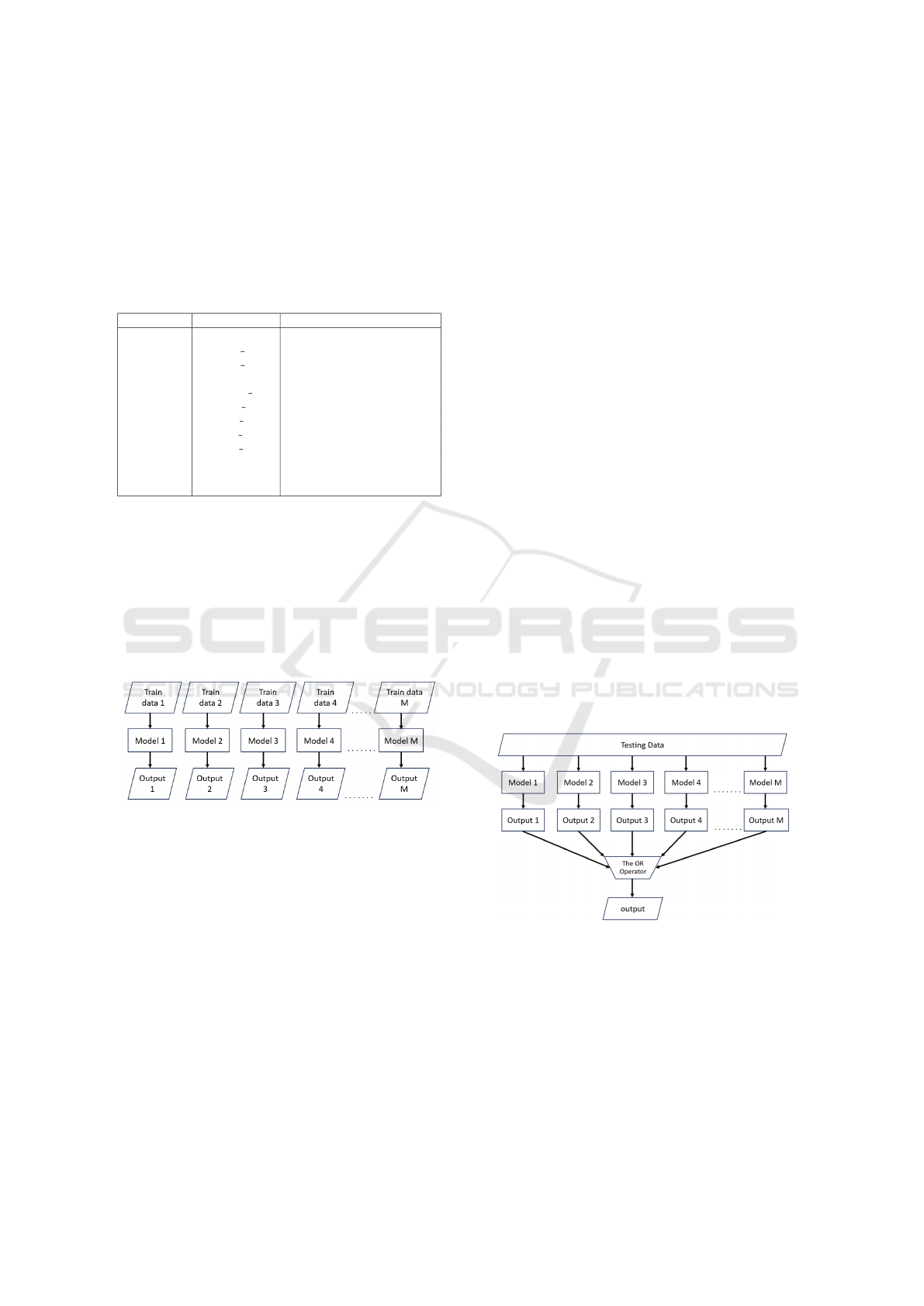
3.3 Individual Models Training
In this stage, because each scenario is treated inde-
pendently, it will be trained individually, as shown in
Figure 1: Training model.
Figure 1 where M represents the total amount of mod-
els trained. We train multiple models to classify the
data
y
m
= f
m
(X
X
X
m
, θ
m
) ; m = ID of model (7)
from the CTU13 dataset, which contains 13 different
scenarios(Garc
´
ıa et al., 2014). Each model is trained
separately for a specific scenario, represented by y
m
in Equation (7), where m indicates the number of the
model. The machine learning method used in this re-
search is the random forest algorithm, represented as
f
m
in Equation (7). Each model in the ensemble con-
sists of 100 trees (θ
m
) with the input data (X
X
X
m
) as
defined in Equation (7). In summary, this process re-
sults in the creation of 13 individual models since the
CTU13 dataset contains 13 scenarios (Garc
´
ıa et al.,
2014).
3.4 Classification by Individual Models
In this stage, our objective is to assess the perfor-
mance of these models. To achieve this, we will uti-
lize the models created in the prior stage and evaluate
their performance using the test set generated during
that stage. We will test each model on all scenarios
within the dataset, covering both those it was trained
on (known scenarios) and those it has never encoun-
tered before (unknown scenarios). This approach al-
lows us to evaluate and compare each model’s bot-
net detection performance in familiar and unfamiliar
scenarios. Consequently, this stage will yield insights
into the adaptability of each model to different scenar-
ios and its effectiveness in detecting botnet activities.
3.5 Integration Methods
Before this, we created and classified 13 models in
the previous two stages. In this stage, we utilized two
integrating techniques that will be mentioned in Sec-
tion 3.5.1 and Section 3.5.2.
3.5.1 Late Integration
The late integrating technique (proposed method) is a
technique that utilizes previously trained models from
the last stage, as illustrated in Figure 1, to predict each
output. The outputs were then integrated using the
Figure 2: Late Integrating Method.
OR operator to obtain a single output, as illustrated
in Figure 2. This integrating technique is also repre-
sented as Equation (8). It takes outputs from multiple
models as input, where m ranges from 1 to M, and
M is the total number of models used for integration.
The output of each model is indicated as y
m
, and we
have used the OR operator to union them and get one
final output, denoted by y as shown in Equation (8).
ICISSP 2024 - 10th International Conference on Information Systems Security and Privacy
370

The final output of late integration is denoted by ˆy, us-
ing Equation (9). If y > 0, it means that the network
traffic flow is classified as a botnet flow, and ˆy will be
considered as 1. Otherwise, ˆy will be considered as 0.
y = y
1
∨ y
2
.... ∨ y
M
=
M
[
m=1
y
m
(8)
ˆy =
(
1, if y > 0
0, otherwise
(9)
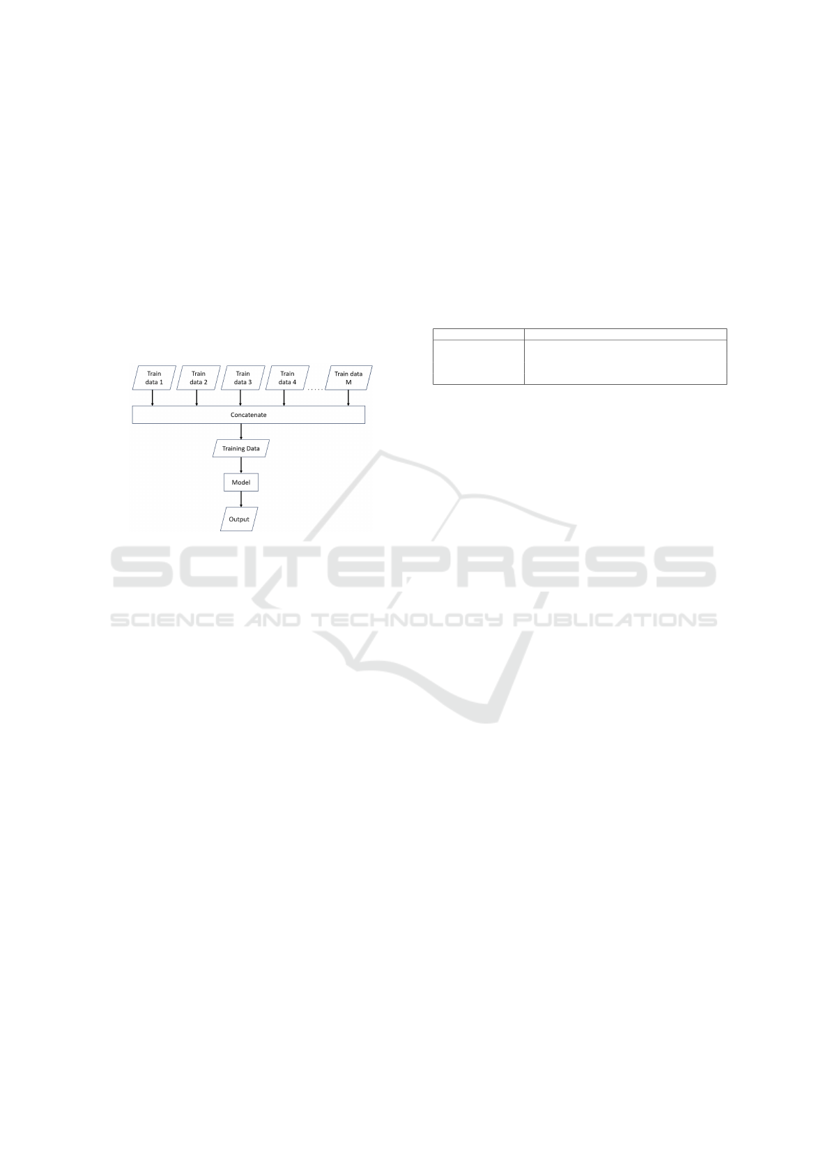
3.5.2 Early Integration
Figure 3: Early Integrate Method.
The early integrating technique is shown in Figure 3.
This technique is quite similar to the late integrating
approach mentioned earlier. It involves concatenat-
ing various scenarios from the dataset before utiliz-
ing them as input to train a single model. Unlike
the late integrating technique, which trains multiple
models, the early integrating technique combines the
data from multiple scenarios to train one model using
the concatenated data. This integrating technique can
also be written as shown in Equation (10). In Equa-
tion (10), X
X
X
M
X
X
X =

X
X
X
1
X
X
X
2
X
X
X
3
. . . X
X
X
M

T
(10)
represents the specific scenario we are referring to for
concatenation. X
X
X represents the concatenated scenar-
ios, which will serve as the input for training a single
model. The purpose of the early integrating technique
is to investigate how effectively a single model can
generalize across different scenarios.
3.6 Evaluation
After completing the tests in the classification by indi-
vidual model and integration method stages, we move
on to evaluating the results using error metric scores.
These scores include:
• The precision score measures the proportion of
actual botnet data that are identified as a botnet
out of all the data that the model classified as a
botnet.
• The recall score indicates the proportion of actual
botnet data that is identified as botnet among all
the real botnet data present in the dataset.
• F1-score tells the harmonic mean between recall
and precision.
Table 4: Classification of evaluation.
Classification Description
True Positive (TP) Botnet flow that got predicted as a botnet
False Positive (FP) Non-botnet flow that got predicted as a botnet
True Negative (TN) Non-botnet flow that got predicted as a non-botnet
False Negative (FN) Botnet flow that got predicted as a non-botnet
where the classification of evaluation is shown in Ta-
ble 4. Although the accuracy score is one of the ma-
jor evaluation methods, we do not use it because the
CTU13 dataset contains a substantial number of non-
botnet flows. The accuracy score calculates the proba-
bility of accurate prediction, and non-botnet flows are
relatively easy to predict. Consequently, it achieves
high accuracy (over 99%) in every scenario. Since
this research aims to minimize false negatives, reduc-
ing instances where the botnet bypasses detection, the
recall score is considered the most important.
4 EXPERIMENTAL SETUP AND
RESULT
4.1 Experimental Setup
We have conducted 2 experiments for each integrating
technique as mentioned in Section 3.5 as follows:
• Known Scenario Approach. All 13 scenarios are
used as input for the training process. To train
each model, we divide the data for each scenario
into a training set (80%) and a test set (20%).
• Unknown Scenario Approach. 12 out of the 13
scenarios are used as input for the training pro-
cess. One scenario is unknown and used as a test
set.
It is important to note that, for both approaches, the
training and testing scenarios remain consistent for
every stage. This consistency ensures a fair and ac-
curate comparison between different approaches.
4.2 Experimental Result
The experimental results for the first part, where we
trained and classified each scenario individually, are
Botnet Detection by Integrating Multiple Machine Learning Models
371

Table 5: Recall Score for Classification by individual models.
Recall scenario ID for training model
Testing Scenario ID 1 2 3 4 5 6 7 8 9 10 11 12 13
1 0.999 0.164 0 0 0 0 0 0 0 0 0 0 0.005
2 0.498 0.999 0 0 0 0 0 0 0 0 0 0 0
3 0 0 0.997 0 0.017 0.001 0 0 0 0 0 0 0
4 0 0 0 0.952 0.094 0.153 0 0 0 0.306 0 0 0.001
5 0 0 0 0 0.997 0 0 0 0.019 0 0 0 0.207
6 0 0 0 0.853 0 0.999 0 0 0 0 0 0 0
7 0 0 0 0 0 0 0.923 0 0 0 0 0 0
8 0 0 0 0 0 0 0 0.958 0 0 0 0 0
9 0 0 0 0 0.003 0 0 0 0.999 0 0 0 0.387
10 0 0 0 0 0.039 0 0 0 0 0.999 0 0 0
11 0 0 0 0.006 0 0 0 0 0 0.058 0.999 0 0
12 0 0 0 0 0 0 0 0 0 0 0 0.977 0
13 0 0 0 0 0.045 0 0 0 0.020 0 0 0 0.999
Table 6: Precision Score for Integration method.
Precision Integration method
Testing Late integration Early integration
Scenario ID KnownL UnknownL KnownE UnknownE
1 0.619 0.967 1 0.999
2 0.614 0.989 1 0.996
3 0.619 0 0.999 0
4 0.626 0.277 1 0
5 0.612 0.022 1 0
6 0.646 0.734 1 0
7 0.605 0 1 1
8 0.640 0 0 0.999
9 0.645 0.993 0.999 0
10 0.596 0.561 0.999 0
11 0.588 0.953 1 0
12 0.634 0 0.989 0
13 0.625 0.003 1 0.894
Table 7: Recall Score for Integration method.
Recall Integration method
Testing Late integration Early integration
Scenario ID KnownL UnknownL KnownE UnknownE
1 0.990 0.182 0.998 0.112
2 0.990 0.381 0.999 0.057
3 0.974 0 0.998 0
4 0.989 0.509 0.941 0
5 0.984 0.197 0.989 0
6 0.990 0.852 0.998 0
7 0.981 0 0.875 0
8 0.978 0 0.953 0
9 0.985 0.419 0.999 0
10 0.989 0.556 0.999 0
11 0.984 0.059 1 0
12 0.980 0 0.970 0
13 0.981 0.061 0.999 0
presented in Table 5. Only recall scores are shown
here because we only want to compare false nega-
tives between the individual model and the integrat-
ing model. Table 5 shows that using one scenario as
the training input for an individual model proved to
be ineffective, resulting in a recall score of 0 for most
scenarios. The poor performance in detecting botnets
across different scenarios can be attributed to vari-
ations in botnet behaviors present in each scenario,
which render models trained on one scenario inade-
Table 8: F1-Score for Integration method.
F1-score Integration method
Testing Late integration Early integration
Scenario ID KnownL UnknownL KnownE UnknownE
1 0.684 0.306 0.999 0.202
2 0.667 0.550 0.999 0.109
3 0.684 0 0.999 0
4 0.735 0.359 0.969 0
5 0.668 0.039 0.994 0
6 0.707 0.789 0.999 0
7 0.664 0 0.933 0
8 0.667 0 0.975 0
9 0.700 0.589 0.999 0
10 0.659 0.101 0.999 0
11 0.646 0.112 1 0
12 0.693 0 0.98 0
13 0.687 0.007 0.999 0
quate for detecting botnets in others.
Then, we applied various integration methods, as
detailed in Section 3.5. The first method, late in-
tegration with known scenarios (KnownL), involves
the collective use of all 13 models. This comprehen-
sive approach exhibited a significant enhancement,
enabling the botnet detection system to identify bot-
net behaviors accurately while minimizing false neg-
atives. As a result, high recall scores are achieved,
as shown in Table 7. Despite checking the general-
ization of this method, we have conducted another
experiment, late integration with unknown scenarios
(UnknownL), as outlined in Section 4.1. The results
for this experimental setup indicate that the recall
score, as displayed in Table 7, remained disappoint-
ingly low. Although it can detect various botnet ac-
tivities, it struggled with four scenarios (Scenario ID
3, 7, 8, and 12) where the recall score was 0, indicat-
ing an inability to detect botnets in these scenarios.
While the precision score in Table 6 and the F1-score
in Table 8 also showed suboptimal outcomes.
On the other hand, early integration with known
scenarios (KnownE) yielded a very high recall score,
with most scenarios achieving a score of over 0.95,
as Table 7 illustrates. Unfortunately, in early integra-
ICISSP 2024 - 10th International Conference on Information Systems Security and Privacy
372

tion with unknown scenarios (UnknownE), most re-
call scores are 0, as Table 7 indicates. While KnownE
achieves a higher recall score than KnownL in most
observed scenarios, it suggests that KnownE may de-
tect botnets better than KnownL for observed scenar-
ios, and UnknownL may outperform UnknownE for
unobserved scenarios. Therefore, considering all sce-
narios, the early integrating technique performs better
in botnet detection than the late integrating technique.
5 CONCLUSION
In this research, we proposed an integrated machine-
learning methodology to tackle the challenges pre-
sented by botnets. Our approach entailed two inte-
gration methods as detailed in Section 3.5, using ran-
dom forests with distinct network traffic characteris-
tics. We combined these models to detect various bot-
net activities.
The experimental results demonstrated the effec-
tiveness of the integration method in detecting various
botnet behaviors, achieving a remarkably low false
negative rate. Consequently, high recall scores, as
indicated in Table 7. This outcome implies that the
proposed method successfully identified a significant
portion of botnet instances, making it challenging for
botnets to bypass detection using this approach.
Nevertheless, we observed a relatively high false
positive rate in the integration method, as indicated by
the F-1 scores in Table 8 and precision scores in Ta-
ble 6. This limitation can be attributed to the similar-
ities between some botnet and non-botnet behaviors.
It’s crucial to emphasize that the success of this botnet
detection methodology hinges on the individual mod-
els’ quality and their capability to achieve a high level
of accuracy in detecting botnet activities. Further im-
provements in model training and refinement are es-
sential to enhance overall detection performance.
Despite the challenges posed by botnets and the
complexities in their detection, our research presents
a promising step forward in mitigating their threat.
The integration method effectively identified various
botnet behaviors, contributing to improving cyberse-
curity defense measures.
In summary, while there is still room for improve-
ment, the integrating machine-learning method pro-
posed in this study opens new avenues for tackling
botnet-related cybersecurity issues. The late integra-
tion method as mentioned in Section 3.5.1 is better
for real-world scenarios since it can be used on-line
at the end of a network trace. This integration method
is a plug-and-play method where a new model that
contains a new type of botnet or new scenarios can
be added anytime. The research has successfully re-
duced false negatives by integrating several machine-
learning models. However, high false positives and
evolving botnet behaviors remain challenges. There-
fore, future work will focus on reducing false pos-
itives by developing and integrating online learning
and incremental updates. Ensuring the system’s ef-
fectiveness will involve maintaining a diverse dataset
that reflects evolving botnet behaviors.
ACKNOWLEDGEMENTS
This research is partially funded by the FY2023
JAIST Grant for Fundamental Research, Japan Ad-
vanced Insitute of Science and Technology.
REFERENCES
Abrantes, R., Mestre, P., and Cunha, A. (2022). Exploring
dataset manipulation via machine learning for botnet
traffic. Procedia Computer Science, 196:133–141. In-
ternational Conference on ENTERprise Information
Systems / ProjMAN - International Conference on
Project MANagement / HCist - International Confer-
ence on Health and Social Care Information Systems
and Technologies 2021.
Bahs¸i, H., N
˜
omm, S., and La Torre, F. B. (2018). Di-
mensionality reduction for machine learning based iot
botnet detection. In 2018 15th International Con-
ference on Control, Automation, Robotics and Vision
(ICARCV), pages 1857–1862.
Binkley, J. and Singh, S. (2006). An algorithm for anomaly-
based botnet detection. In Workshop on Steps to Re-
ducing Unwanted Traffic on the Internet.
Garc
´
ıa, S. (2014). Identifying, Modeling and Detecting Bot-
net Behaviors in the Network. PhD thesis.
Garc
´
ıa, S., Grill, M., Stiborek, J., and Zunino, A. (2014).
An empirical comparison of botnet detection methods.
Computers & Security, 45:100–123.
Haddadi, F. and Zincir-Heywood, A. N. (2017). Bot-
net behaviour analysis: How would a data analytics-
based system with minimum a priori information per-
form? International Journal of Network Management,
27(4):e1977. e1977 nem.1977.
Hegna, A. (2010). Visualizing spatial and temporal dynam-
ics of a class of irc-based botnets. Master’s thesis,
Institutt for telematikk.
Kuo, C.-C., Tseng, D.-K., Tsai, C.-W., and Yang, C.-S.
(2021). An effective feature extraction mechanism for
intrusion detection system. IEICE Transactions on In-
formation and Systems, E104.D(11):1814–1827.
Rajab, M. A., Zarfoss, J., Monrose, F., and Terzis, A.
(2006). A multifaceted approach to understanding
the botnet phenomenon. In ACM/SIGCOMM Internet
Measurement Conference.
Botnet Detection by Integrating Multiple Machine Learning Models
373