
Investigation into the Training Dynamics of Learned Optimizers
Jan Sobotka, Petr
ˇ
Sim
´
anek and Daniel Va
ˇ
sata
Faculty of Information Technology, Czech Technical University in Prague, Th
´
akurova 9, Prague, Czech Republic
fi
Keywords:
Learning to Optimize, Meta-Learning, Optimization.
Abstract:
Optimization is an integral part of modern deep learning. Recently, the concept of learned optimizers has
emerged as a way to accelerate this optimization process by replacing traditional, hand-crafted algorithms
with meta-learned functions. Despite the initial promising results of these methods, issues with stability and
generalization still remain, limiting their practical use. Moreover, their inner workings and behavior under
different conditions are not yet fully understood, making it difficult to come up with improvements. For
this reason, our work examines their optimization trajectories from the perspective of network architecture
symmetries and parameter update distributions. Furthermore, by contrasting the learned optimizers with their
manually designed counterparts, we identify several key insights that demonstrate how each approach can
benefit from the strengths of the other.
1 INTRODUCTION
In the last decade, the field of machine learning has
undergone many trends, the most significant being
the replacement of manual feature engineering with
learned features. Relatively recently, a similar per-
spective has been applied to optimization, the driving
force behind deep learning. Specifically, the subfield
of meta-learning called learning to optimize (L2O)
has the ambitious goal of learning the optimization
itself, more or less replacing the hand-engineered al-
gorithm approach.
There is a substantial body of literature devoted to
learning to optimize with available gradient informa-
tion. These works try to learn the ”gradient descent-
like” method to optimize the parameters (weights and
biases) of neural networks. The approaches range
from learning adaptive step size (learning rate) to
learning the whole gradient descent algorithm with re-
current neural networks (Andrychowicz et al. (2016),
Lv et al. (2017), Metz et al. (2020), Metz et al. (2021),
Simanek et al. (2022)).
Compared to the relatively long history of hand-
engineered optimizers, where extensive research into
the theory, together with many empirical findings,
informed numerous advances (momentum Polyak
(1964), AdaGrad Duchi et al. (2011), RMSProp
Tieleman et al. (2012), Adam Kingma and Ba
(2017)), the field of learning to optimize is in its
nascent stages. Many fundamental questions remain
unanswered, and an extensive investigation into the
training dynamics of learned optimizers is still lack-
ing, which hinders well-informed development and
further progress of the whole field. This is especially
important since these methods have been shown to be
brittle, difficult to scale, and relatively ineffective at
generalizing across diverse problems.
Additionally, it might be possible to improve man-
ually engineered optimization algorithms by noticing
which strategies L2O has found to be useful. In other
words, research on hand-designed and learned opti-
mizers can be mutually beneficial.
In light of the aforementioned lack of understand-
ing and our desire to improve traditional optimizers,
we empirically study various properties of the opti-
mization trajectories. Specifically, we 1) analyze the
impact of symmetries introduced by network archi-
tectures; 2) examine the heavy-tailedness of noise in
the predicted parameter updates; 3) investigate the up-
date covariance, and lastly; 4) inspect the progression
of the update size.
Our results show several major differences as well
as similarities between the training dynamics under
traditional and learned optimizers. Moreover, we no-
tice close parallels to the recently proposed optimizer
Lion (Chen et al., 2023) and shed more light on the
strengths of these two approaches.
In particular, our experiments demonstrate that
similarly to Lion, learned optimizers break the ge-
ometric constraints on gradients that stem from ar-
Sobotka, J., Šimánek, P. and Vašata, D.
Investigation into the Training Dynamics of Learned Optimizers.
DOI: 10.5220/0012317000003636
Paper published under CC license (CC BY-NC-ND 4.0)
In Proceedings of the 16th International Conference on Agents and Artificial Intelligence (ICAART 2024) - Volume 2, pages 135-146
ISBN: 978-989-758-680-4; ISSN: 2184-433X
Proceedings Copyright © 2024 by SCITEPRESS – Science and Technology Publications, Lda.
135
chitectural symmetries and that deviations from these
constraints are significantly larger than those ob-
served with previous optimizers like Adam or SGD.
In the case of learned optimizers, we observe that a
large deviation from these geometric constraints al-
most always accompanies the initial rapid decrease in
loss during optimization. More importantly, regular-
izing against it severely damages performance, hint-
ing at the importance of this freedom in L2O parame-
ter updates.
Furthermore, by studying the noise and covariance
in the L2O parameter updates, we also demonstrate
that, on the one hand, L2O updates exhibit less heavy-
tailed stochastic noise, and, on the other hand, the
variation in updates across different samples is larger.
The paper is organized as follows. In Section 2,
learned optimizers and the Lion optimizer are intro-
duced. Then Section 3 describes the theoretical anal-
ysis of symmetries, gradient geometry, stochastic gra-
dient noise, and update covariance. This, in turn,
leads to a series of experiments presented in Section 4
followed by a discussion in Section 5. Lastly, Section
6 connects our work to previous studies and shows
promising parallels.
2 BACKGROUND
Let us start by explaining the learning to optimize
method, which is the main subject of our study, and
then follow with the recently introduced Lion opti-
mizer.
2.1 Learning to Optimize
The primary task is to minimize a given function L(θ)
by optimizing its vector of parameters θ. We focus
primarily on first-order optimization methods, where
at each step t of the algorithm, the optimizer has ac-
cess to the gradient ∇L(θ
t
) and suggests an update g
t
to get θ
t+1
as
θ
t+1
= θ
t
+ g
t
. (1)
Our approach follows Andrychowicz et al. (2016).
The core idea is to use a recurrent neural network M,
parameterized by φ, that acts as the optimizer. Specif-
ically, at each time step t, this network takes its hid-
den state h
t
together with the gradient ∇L(θ
t
) and pro-
duces an update g
t
and a new hidden state h
t+1
,
[g
t
, h
t+1
] = M
∇
θ
L(θ
t
), h
t
, φ
. (2)
The sequence obtained by (1) then aims to con-
verge to a local minimum of L. Therefore, M is called
the optimizer, or meta-learner, and L(θ) is called the
optimizee.
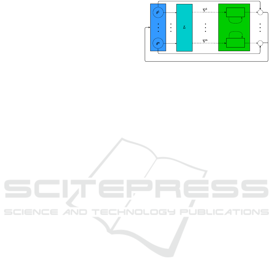
LSTM
1
LSTM
n
+
+
Figure 1: Single optimization step of L2O.
The parameters φ of the optimizer M are learned
by stochastic gradient descent and updated every u-th
training step where the hyper-parameter u is called the
unroll. The loss of the optimizer is the expectation of
the weighted unrolled trajectory of the optimizee,
L (φ) = E
L
u
∑
τ=1
w
τ
L(θ
τ+ ju−1
) (3)
where E
L
is the expectation with respect to some dis-
tribution of optimizee functions L and w
τ
are weights
that are typically set to 1. Additionally, j denotes the
number of previously unrolled trajectories; therefore,
( j + 1)-th unrolled trajectory corresponds to training
steps t = ju, ju + 1, ..., ( j + 1)u −1. In practice, there
is often only one optimizee function L, so the expec-
tation in (3) is removed.
In addition to updates of φ along a single opti-
mizee training (an inner loop), there is also an outer
loop where the entire optimizee training is restarted
from some initial θ
t=0
while the parameters φ con-
tinue to learn. In particular, the outer loop takes place
only during the meta-training phase, where the main
goal is to learn a good set of parameters φ. Evalu-
ation of the learned optimizer then happens in what
is sometimes called meta-testing where φ is fixed and
only the optimizee’s parameters θ are updated.
In practice, when there are several thousand or
more parameters in θ, applying a general recurrent
neural network is almost impossible. The authors in
Andrychowicz et al. (2016) avoid this issue by imple-
menting the update rule coordinate-wise using a two-
layer LSTM network with shared parameters. This
means that the optimizer M is a small network with
multiple instances operating on each parameter of the
optimizee separately while sharing its parameters φ
across all of them. A visualization of a single opti-
mization step is presented in Figure 1.
We refer the reader to Andrychowicz et al. (2016)
for further algorithmic details and preprocessing.
2.2 Lion Optimizer
By applying program search techniques to the discov-
ery of optimization algorithms, the authors of Chen
ICAART 2024 - 16th International Conference on Agents and Artificial Intelligence
136
et al. (2023) came up with a simple yet highly ef-
fective adaptive algorithm called Lion (EvoLved Sign
Momentum). The major distinction between Lion and
other adaptive optimizers lies in its uniform update
magnitude for each parameter, calculated through the
sign operation. Remarkably, the authors demon-
strated that this relatively simple optimization algo-
rithm can outperform standard optimizers, such as
Adam or Adafactor, across a wide range of bench-
marks.
A single step of the Lion optimizer starts with a
standard weight decay step with a strength parameter
λ. Then, Lion updates the parameters with the sign
of the interpolation between the current gradient and
momentum. The size of the step is determined by a
learning rate η and the interpolation is controlled by
an exponential moving average (EMA) factor β
1
. Fi-
nally, an update of the EMA is carried out using the
EMA factor β
2
.
According to the authors, the sign operation in
Lion introduces noise into the updates, which serves
as a form of regularization. Empirical observations by
the authors and previous studies Foret et al. (2021),
Neelakantan et al. (2015) suggest that this noise can
contribute to improved generalization. Additionally,
their analysis indicated that Lion’s updates generally
exhibit a larger norm compared to those of Adam.
3 METHODS
3.1 Symmetries and Gradient Geometry
In this section, we formalize the notion of differen-
tiable symmetries, discuss the associated geometric
properties of gradients in the context of neural net-
works, and present important examples.
3.1.1 Differentiable Symmetries
Symmetries of a function express its property of be-
ing invariant under a certain group of transformations.
When these transformations are differentiable, we call
them differentiable symmetries. In this paper, we con-
sider symmetries of loss functions, and the subject of
transformations in our case are the neural network’s
parameters.
More formally, a function f (θ) where θ ∈R
n
pos-
sesses a differentiable symmetry if it is invariant un-
der the differentiable action ψ : R
n
×G → R
n
of a
group G on the function’s argument space. In other
words, for all θ and all α ∈ G, the output of the func-
tion does not change:
f (ψ(θ, α)) = f (θ). (4)
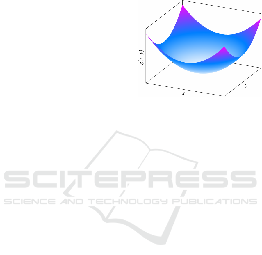
Figure 2: Example function g(x, y) = x
2
+ y
2
.
Note that our topic of interest is different from the
work on equivariant neural networks, where the sym-
metry groups act on the input space, output space, and
hidden feature spaces. Specifically, their focus is on
the equivariance or invariance of y = f
θ
(x) with re-
spect to x and y, but in the following sections, we
are interested in symmetries acting on the parameter
space instead.
3.1.2 Geometric Constraints on Gradients
Let us start with an intuitive example to introduce the
concept of gradient geometry. Consider the function
g(x, y) = x
2
+ y
2
depicted in Figure 2 that possesses
rotational symmetry
ψ(x, y, α) =
cosα −sinα
sinα cosα
x
y
, (5)
i.e. rotating around the origin by some angle α leaves
the output of g unchanged.
Taking the partial derivative at the identity α = 0,
we get
∂
α
ψ
α=0
=
−y
x
, (6)
where ∂
α
ψ
α=0
is the vector field that generates the
symmetry. Taking the gradient of g at (x, y) yields
∇g = 2
x
y
(7)
Hence, the gradient is perpendicular to the vector
field:
⟨∇g, ∂
α
ψ
α=0
⟩ = 0 for all x, y. (8)
See Figure 3 for a depiction of this geometrical prop-
erty.
As will be now easily shown, such perpendicular-
ity is not specific for the presented example, but it
Investigation into the Training Dynamics of Learned Optimizers
137
x
y
x
y
x
y
Figure 3: Gradient geometry for the function g(x, y) =
x
2
+y
2
. Left: Directions of the gradient ∇g. Middle: Direc-
tions of the vector field ∂
α
ψ
α=0
that generates the symme-
try. Right: Orthogonality of the gradient and the symmetry-
generating vector field.
holds generally. Let us assume that f is almost ev-
erywhere differentiable. By taking the derivative with
respect to α at the identity α = I ∈ G of both sides of
(4) and using the chain rule of differentiation, we get
∇ f , ∂
α
ψ
α=I
= 0, (9)
which implies that for all θ, the gradient ∇ f whenever
exists is perpendicular to the vector field ∂
α
ψ
α=I
that
generates the symmetry.
Similar relationships hold for the Hessian matrices
as can be found in Kunin et al. (2021) together with
formal proofs and a more detailed discussion of the
above.
Since our analysis focuses on learning to optimize
methods, we investigate how the predicted parame-
ter updates adhere to the constraints on gradients and
how deviations from these geometric constraints com-
pare to those of SGD, Adam, and Lion.
Additionally, part of our analysis includes regu-
larization of learned optimizers during meta-training
against the aforementioned deviations. In such cases,
we calculate the absolute deviations for each pre-
dicted update during meta-training using the opti-
mizee’s detached parameters and include these abso-
lute deviations as part of the optimizer’s loss.
A description of the three symmetries considered,
along with methods for calculating deviations from
the associated geometric constraints, is provided be-
low.
Translation Symmetry. In this paper, translation
symmetry refers to the invariance of a function to
action ψ(θ, α) : θ 7→ θ + αξ, where ξ ∈ R
n
is some
constant vector and α ∈ R. We will consider only
cases where ξ =
X
, which is the indicator vector for
some subset X of {1, ..., n}. An example is the vector
{1,3}
= (1, 0, 1, 0, . . . , 0). From (9), we get
∇ f , ∂
α
ψ
α=0
=
∇ f ,
X
= 0. (10)
In other words, the gradient is orthogonal to the indi-
cator vector.
Let us have a subset X = {i
1
, i
2
, . . . , i
k
} of
{1, ..., n} and denote by ∇
θ
X
f the gradient of f with
respect to a subset of its arguments given by θ
X
=
(θ
i
1
, θ
i
2
, . . . , θ
i
k
) ∈
k
. Then, we may rewrite the pre-
vious orthogonality as
∇ f ,
X
=
∇
θ
X
f ,
= 0, (11)
where = (1, . . . , 1).
In the context of deep learning, the translation
symmetry is present in the softmax function σ
i
(z) =
e
z
i
Σ
j
e
z
j
with z = W x + b. Shifting any column W
:,i
or the
bias vector b by a real constant leaves the output of
the softmax unchanged. Therefore, the softmax func-
tion is invariant under translation, and this symmetry
induces from (11) the following gradient property:
∇
W
:,i
L,
=
∇
b
L,
= 0, (12)
where we denote by L the loss function.
The equation above provides us with a simple way
to calculate absolute deviation from this symmetry-
induced constraint as follows:
g
b
(∇L),
+
∑
i
g
W
:,i
(∇L),
, (13)
where the function g denotes the update rule of an op-
timizer with the corresponding components g
b
, g
W
:,i
,
and the index i iterates over all the columns of W .
Rescale Symmetry. Rescale symmetry is in our
case defined by the group GL
+
1
(R) and the action
ψ(θ, α) : θ 7→ a
X
1
(α) ⊙a
X
2
(α
−1
) ⊙θ, where X
1
and
X
2
are two disjoint subsets of {1, ..., n}, α ∈ (0, +∞),
a
X
1
(α) = + (α − 1)
X
1
, and ⊙ is the element-
wise multiplication. An example of the notation is
a
{1,3}
(α) = (α, 1, α, 1, . . . , 1). Function f possesses
rescale symmetry if f (θ) = f (ψ(θ, α)) for all α ∈
GL
+
1
(R). Taking similar steps as before, this sym-
metry implies gradient orthogonality as
∇ f , ∂
α
ψ
α=1
=
∇ f , θ⊙
X
1
−θ ⊙
X
2
= 0. (14)
Full formal proofs can be found in Kunin et al. (2021).
Interestingly, the rescale symmetry is present at
every hidden neuron of networks with continuous, ho-
mogeneous activation functions such as ReLU and
Leaky ReLU. A simple illustration of this comes
from considering a single neuron’s computational
path w
2
σ(w
T
1
x + b) and noticing that scaling w
1
and
b by a real constant and w
2
by its inverse has no effect
since the constants can be passed through the activa-
tion function, canceling their effect. Thus, the gradi-
ent constraints in this case are
∇
w
1
L, w
1
+
∇
b
L, b
−
∇
w
2
L, w
2
= 0. (15)
Absolute deviation of the optimizer’s updates
given by g from the rescale symmetry constraints can
be therefore calculated as
g
w
1
(∇L), w
1
+
g
b
(∇L), b
−
g
w
2
(∇L), w
2
.
(16)
ICAART 2024 - 16th International Conference on Agents and Artificial Intelligence
138

Scale Symmetry. Scale symmetry can be defined
by the group GL
+
1
(R) and the action ψ(θ, α) : θ 7→
a
X
(α) ⊙ θ, where the notation is the same as for
the rescale symmetry. Given this definition, a func-
tion possesses scale symmetry if f (θ) = f (ψ(θ, α)) =
f (α
X
⊙θ) for all α ∈ GL
+
1
(R). The gradient orthog-
onality arising from this symmetry is
∇ f , ∂
α
ψ
α=1
=
∇ f , θ ⊙
X
=
∇
θ
X
f , θ
X
= 0
(17)
i.e. the gradient of the function is everywhere perpen-
dicular to the parameter vector itself.
Batch normalization, as used in deep learning, has
this scale invariance during training. To see this, con-
sider the incoming weights w ∈ R
d
and bias b ∈ R
of a neuron with batch normalization
z−¯z
√
var(z)
, where
z = w
T
x + b, ¯z is the sample average, and var(z) is
some standard estimation of variance. Scaling w and
b by a non-zero real constant has no effect on the out-
put since it factors from z, ¯z, and
p
var(z) canceling
the effect. Thus, w and b observe scale symmetry in
the loss, and their gradients satisfy
⟨∇
w
L, w⟩+ ⟨∇
b
L, b⟩ = 0. (18)
More details can be found in Ioffe and Szegedy (2015)
and Kunin et al. (2021).
Therefore, we can calculate the absolute deviation
of the updates given by g from the scale symmetry
constraints as
⟨g
w
(∇L), w⟩+ ⟨g
b
(∇L), b⟩
. (19)
3.2 Stochastic Gradient Noise and
α-Stable Distributions
3.2.1 Stochastic Gradient Noise
Stochastic gradient noise refers to the fluctuations in
the gradient of the loss function. This noise can be
characterized by the gradient noise vector, defined as
U
k
= ∇L
k
−∇L, (20)
where ∇L
k
is the k-th mini-batch gradient and ∇L is
the full-batch gradient of the loss function.
Although many theoretical works have assumed
U
k
to be Gaussian with independent components, the
authors of Simsekli et al. (2019) have shown that
this is not entirely the case. Their theory suggested
that the gradient noise converges to a heavy-tailed α-
stable random variable and proposed a novel analy-
sis of SGD, which their experiments showed to be
more suitable. Specifically, in a series of experiments
with common deep learning architectures, the gradi-
ent noise exhibited a highly non-Gaussian and heavy-
tailed distribution.
More importantly, they proved that gradient noise
with heavier tails increases the probability of ending
up in a wider basin of the loss landscape, an indication
of better generalization (Hochreiter and Schmidhuber
(1997)).
3.2.2 Symmetric α-Stable Distributions
One can view the symmetric α-stable (SαS) distri-
bution as a heavy-tailed generalization of a centered
Gaussian distribution. The SαS distributions are de-
fined through their characteristic function
X ∼ SαS(σ) ⇐⇒ E
e
iωX
= e
−|σω|
α
. (21)
In general, the probability density function does
not have a closed-form formula, but it is known that
the density decays with a power law tail like |x|
−α−1
where α ∈ (0, 2] is called the tail-index: as α gets
smaller, the distribution has a heavier tail.
Under the assumption of the same tail-index for all
components of the gradient noise and of the parameter
update noise defined by
U
k
= g
k
−g, (22)
where g
k
is the k-th mini-batch parameter update and
g is the full-batch update, we estimate the tail-index
α of the distribution of the gradient noise components
and the parameter update noise components using the
estimator introduced in Mohammadi et al. (2015) and
specifically its implementation from Simsekli et al.
(2019).
3.3 Update Covariance
To further investigate the noise in the mini-batch pa-
rameter updates for different optimizers, we study the
magnitude of their variation across different samples.
We do so by considering the update covariance matrix
K =
1
N
N
∑
i=0
(g
i
−g)(g
i
−g)
T
, (23)
where g
i
is the parameter update on the sample x
i
, g is
the full-batch update, and N is the number of training
samples.
Computing and storing K in memory is expensive
due to the quadratic cost in the number of parame-
ters. However, since we want to analyze the magni-
tude of the deviations of the parameter updates from
the full-batch update, it is sufficient to determine only
the largest eigenvalue of K.
To address this, we use the mini-batch updates as
follows. We begin by sampling L mini-batch update
of size M and compute the corresponding L ×L Gram
matrix K
M
with entries
K
M
i, j
=
1
L
⟨g
i
−g, g
j
−g⟩, (24)
Investigation into the Training Dynamics of Learned Optimizers
139
where g
i
is the i-th mini-batch update and g is the
estimation of the full-batch update based on the L
mini-batches (in our analysis, we use L = 93). Sub-
sequently, we find the maximum eigenvalue of K
M
using the power iteration method. The empirical find-
ings of the authors of Jastrzebski et al. (2020) demon-
strate that the largest eigenvalue of K
M
approximates
the largest eigenvalue of K quite well.
4 EXPERIMENTS
All our meta-training is performed on feed-forward
neural network optimizees with 1 hidden layer of 20
neurons with either sigmoid, Leaky ReLU, or batch
normalization followed by ReLU. We put the soft-
max activation function at the output and train the
optimizees on the MNIST classification task with the
cross-entropy loss function and batch size of 128. We
set unroll to 20 iterations, learning rate to 0.001, and
perform meta-training for 50 epochs, each consisting
of 20 separate optimization runs with the maximum
iteration number of 200.
During meta-testing, we evaluate L2O on the op-
timizee architectures from meta-training as well as on
larger networks described in each experiment sepa-
rately.
For SGD, Adam, and Lion, by performing a hy-
perparameter search, we chose a learning rate of 0.1
and momentum of 0.9 for SGD, a learning rate of 0.05
for Adam, and learning rates 0.001, 0.005, 0.01 for
sigmoid, Leaky ReLU, and ReLU with batch normal-
ization, respectively, for Lion.
4.1 Breaking the Geometric Constraints
To assess the importance of learned optimizers being
free from the geometric constraints that might bind
classical optimizers, we follow a two-step procedure.
First, we measure the deviations of L2O from the
aforementioned geometric constraints for the trans-
lation, rescale, and scale symmetries. Second, we
regularize the learned optimizer during meta-training
against breaking these constraints and observe its ef-
fects on the performance during meta-testing. The
goal is to better understand the difference between
the optimization trajectories of L2O and classical op-
timizers through the lens of symmetries in the opti-
mizee architecture.
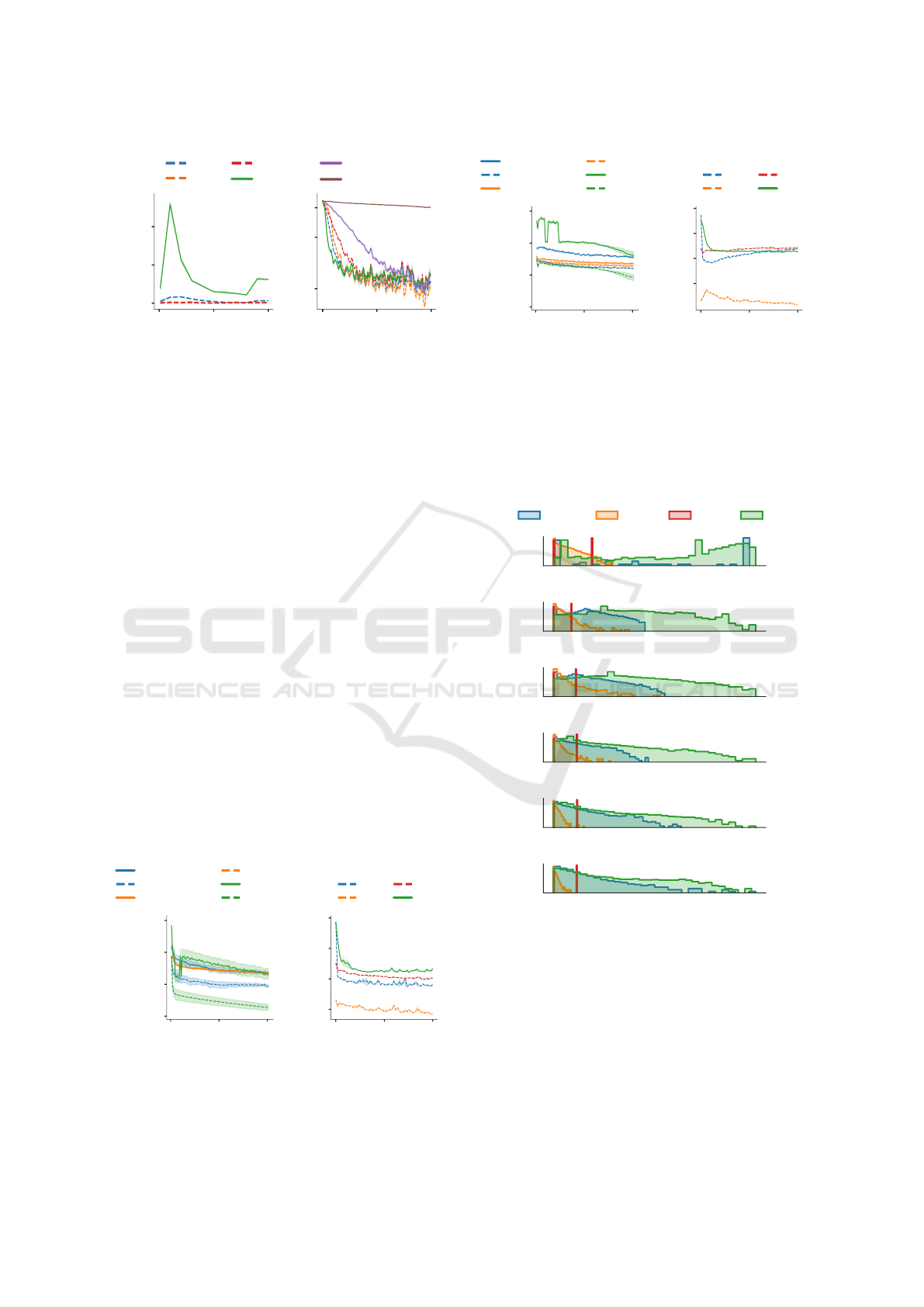
Deviations from the Constraints. We meta-train
and subsequently meta-test L2O on the aforemen-
tioned optimizee models and track the progression of
0 50 100
Absolute deviation
Adam SGD Lion L2O
0 50 100
Iteration Iteration
0
20
40
60
0
20
40
Figure 4: Deviations from the geometric constraints. Left:
Rescale symmetry breaking on the Leaky ReLU optimizee.
Right: Scale symmetry breaking on the optimizee with
batch normalization and ReLU.
the deviations of parameter updates from the geomet-
ric constraints. Additionally, we compare the devi-
ations of hand-engineered optimizers such as SGD,
Adam, and Lion.
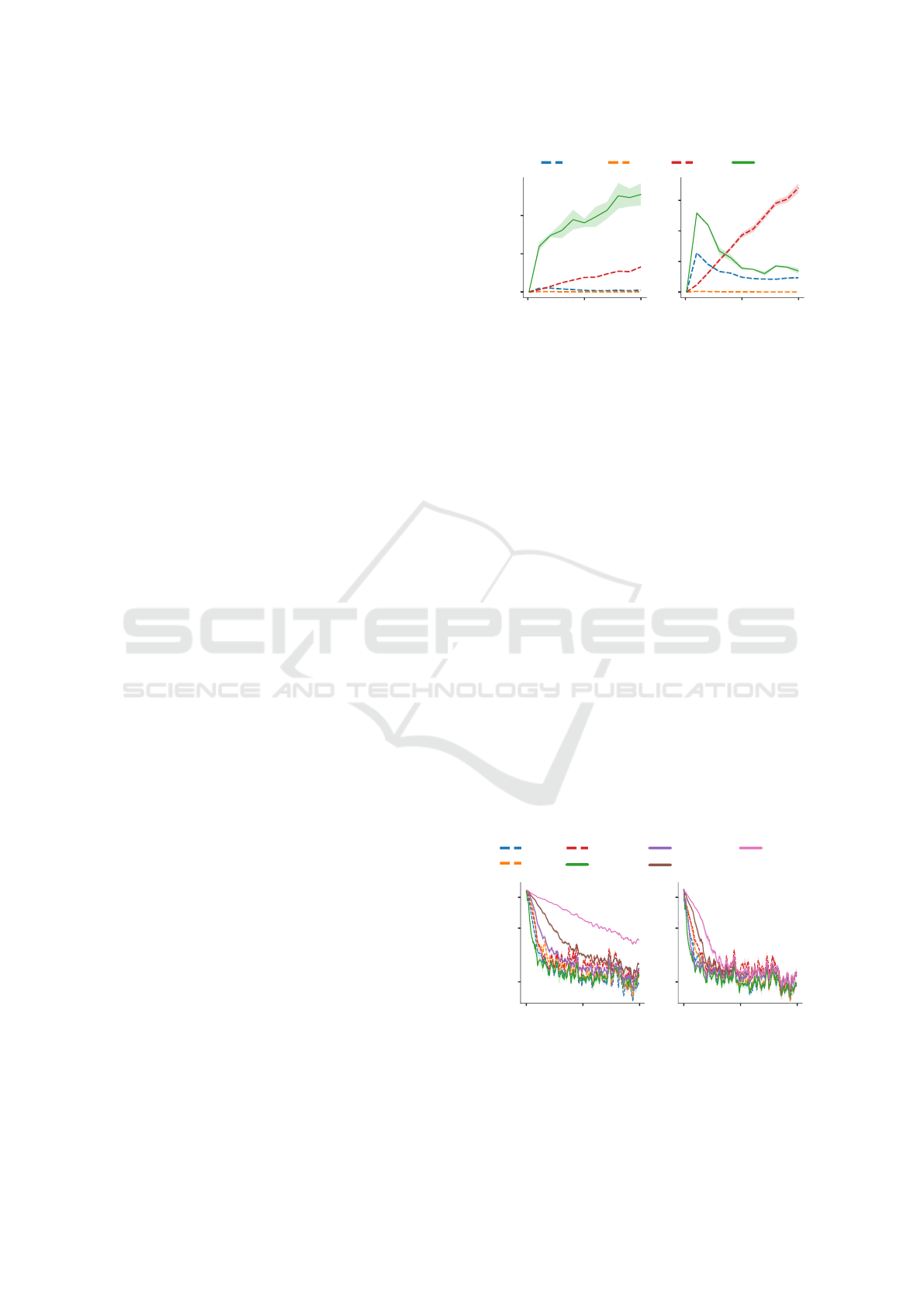
As can be seen in Figure 4, where L2O was meta-
trained on optimizees with Leaky ReLU and ReLU
with batch normalization, the deviations from the ge-
ometric constraints from the rescale and scale symme-
tries are mostly larger than those of SGD and Adam.
But most strikingly, the increase in this symmetry
breaking is largest for L2O at the beginning of op-
timization, whereas for Lion, it increases more grad-
ually and achieves higher values later.
Symmetry Breaking Regularization. To get a
deeper insight into how L2O leverages the freedom of
parameter updates, we meta-train with an additional
regularization loss that penalizes the absolute size of
the L2O’s update deviations from the geometric con-
straints on gradients. The performance for various
regularization strengths β is shown in Figure 5.
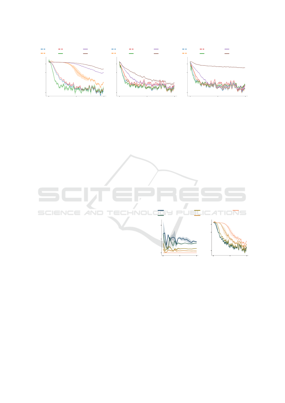
Interestingly, as regularization increases, the
L2O’s optimization speed significantly drops. This
0 100
Iteration Iteration
200 0 100 200
Train loss (log scale)
0.3
1
2
0.3
1
2
Adam
SGD
Lion
L2O,β=0
L2O,β=0.1
L2O,β=0.5
L2O,β=1
Figure 5: Performance after the symmetry breaking regu-
larization. Left: Rescale symmetry breaking regularized on
the Leaky ReLU optimizee. Right: Scale symmetry break-
ing regularized on the optimizee with ReLU and batch nor-
malization.
ICAART 2024 - 16th International Conference on Agents and Artificial Intelligence
140
Adam
SGD
Lion
L2O, β=0.0
L2O, β=0.1
L2O, β=0.5
0 100 200
Iteration
0.2
1
2
Train loss (log scale)
Adam
SGD
Lion
L2O, β=0.0
L2O, β=0.1
L2O, β=0.5
0 100 200
Iteration
0.2
1
2
Train loss (log scale)
Adam
SGD
Lion
L2O, β=0.0
L2O, β=0.1
L2O, β=0.5
0 100 200
Iteration
0.2
1
2
Train loss (log scale)
Figure 6: Effects of regularization strength β on the performance of L2O on novel optimizee architectures. Left: L2O meta-
trained on the Leaky ReLU optimizee with regularization against the rescale symmetry breaking and then meta-tested on
5x wider and 2x deeper optimizee network with sigmoid. Middle: L2O meta-trained on the Leaky ReLU optimizee with
regularization against the rescale symmetry breaking and then meta-tested on ReLU with batch normalization. Right: L2O
meta-trained on the sigmoid optimizee with regularization against the translation symmetry breaking and then meta-tested on
ReLU with batch normalization.
observation reiterates the interesting L2O character-
istic that its optimization trajectories do not escape
the symmetry-induced equivalent parameter combi-
nations as gradient would, but rather take a route more
aligned with the level sets of the loss landscape. Such
a search for a better starting point for the next step
might be related to the symmetry teleportation pre-
sented in Zhao et al. (2022), where the authors per-
formed loss-invariant symmetry transformations of
the parameters to find combinations with a steeper
gradient. Given that L2O is meta-trained and its pre-
dicted parameter updates are history-dependent, it is
an interesting topic for future study to analyze this
connection further.
The same observation for the effect of regulariza-
tion can be made for most of the optimizee architec-
tures on which L2O was not meta-trained (Figure 6).
Results for L2O meta-trained on the optimizee with
sigmoid activation function can be found in the Ap-
pendix.
Symmetry Breaking and Performance of Tradi-
tional Optimizers. We can also relate the symme-
try breaking of classical hand-designed optimizers to
their performance. Specifically, by interpolating be-
tween the optimization steps of SGD and Lion, we
analyze how the change in symmetry breaking of this
combined optimizer coalesces with the change in its
performance.
Figure 7 shows how the Lion-SGD interpolation
maps onto the deviations from the symmetry con-
straints (left) and the performance (right). λ
L
refers
to the interpolation coefficient in
g
Lion-SGD
= λ
L
·g
Lion
+ (1 −λ
L
) ·g
SGD
, (25)
where g’s denote the parameter updates of the corre-
sponding optimizers. The optimizee, in this case, is
a feed-forward neural network with 2 hidden layers
of 100 neurons with sigmoid activation function (the
same as in Figure 6 on the left).
Similarly to the earlier observation that the regu-
larization of L2O symmetry breaking hinders its per-
formance, we see that the increasing symmetry break-
ing of Lion-SGD correlates with an increase in perfor-
mance. This indicates that breaking the strict geomet-
ric constraints is beneficial not only for L2O but also
for more traditional, manually designed optimization
algorithms.
0 100
200
Train loss (log scale)
Absolute deviation
0 100 200
0.2
Iteration Iteration
0
0.5
1.0
1
2
Lion
Lion-SGD, λ
L
=0.5
Lion-SGD, λ
L
=0.25
Lion-SGD, λ
L
=0.1
SGD
Figure 7: Deviations from the geometric constraints and the
performance of the Lion-SGD optimizer. Left: Translation
symmetry breaking on the sigmoid optimizee from Figure 6
on the left. Right: Training loss on the same optimizee.
4.2 Heavy-Tailed Distribution of
Gradient and Parameter Update
Noise
In this section, we investigate the progression of the
estimated tail-index α of the gradient noise compo-
nents and the parameter update noise components for
different optimizers. With lower values of α indicat-
Investigation into the Training Dynamics of Learned Optimizers
141

10
3
10
2
10
1
Largest eigenvalue
Adam
SGD
Lion
L2O
0 500
Iteration
1000
0 500
Iteration
1000
0.5
0.6
0.7
0.8
0.9
Alpha estimate
Adam - updates
Adam - gradients
SGD - updates
SGD - gradients
L2O - updates
L2O - gradients
Figure 8: Heavy-tailedness and update covariance. Left: α
estimates for the gradient and update noise on the Leaky
ReLU optimizee. Right: Largest eigenvalue of the update
covariance on the Leaky ReLU optimizee.
ing a more heavy-tailed distribution of noise of gra-
dients and updates, we are particularly interested in
comparing how the suggested parameter updates from
SGD, Adam, and L2O evolve over a training run.
The results for L2O meta-trained on the Leaky
ReLU optimizee are shown in Figure 8 (left).
First, we see that the estimates of α for L2O pa-
rameter updates are much higher than for the gradi-
ents, implying that the distribution of the noise in its
updates is less heavy-tailed than that of the gradient.
This shows that L2O effectively attenuates the heavy-
tail portion of deviations in the gradient estimates on
its input, taking a less jittery optimization trajectory.
Moreover, one can see that except for a few drops of
α at the beginning of training, the noise in the updates
from L2O is generally less heavy-tailed than the up-
dates from Adam or SGD. Given the previous studies
(Simsekli et al. (2019)) on the benefits of stochastic
gradient noise for generalization, future developments
of the L2O methods might want to take this obser-
vation of less heavy-tailed update noise into account
when troubleshooting optimizee generalization gaps.
Since our experiments are performed on a rather sim-
ple task of MNIST classification, we do not encounter
such problems. Results for the other settings can be
found in the Appendix.
Second, since L2O was meta-trained only on
training runs of 200 iterations, we observed that the
loss in the meta-testing on sigmoid and ReLU with
batch normalization optimizees starts to increase after
around the 500th iteration. This inability to general-
ize to longer training sequences accurately correlates
with decreasing α estimates for L2O’s parameter up-
dates and gradients on these two optimizee architec-
tures as can be seen in the Appendix. With the Leaky
ReLU optimizee network in Figure 8, the training loss
does not increase as for the other two optimizee archi-
tectures and so the α estimates are kept at around the
same value even after the 500th iteration.
4.3 Update Covariance
As described in Methods (Section 3.3), we want to
investigate the noise (variation) in the mini-batch pa-
rameter updates for different optimizers. We follow
the same setup as in the previous experiments. The
results for update covariance of all considered opti-
mizers on the Leaky ReLU optimizee are shown in
Figure 8 (right). Results for the other optimizees can
be found in the Appendix.
Interestingly, once again, we observe a similar rel-
ative ordering among the considered optimizers. In
this case, the variation in updates across different
samples appears to be the lowest for SGD, followed
by Adam, Lion, and, finally, the largest variation is
observed for L2O.
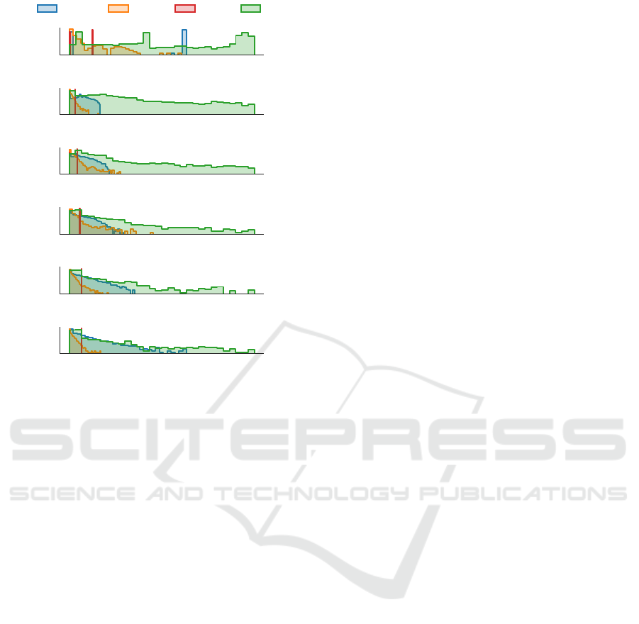
4.4 Update Histograms
To compare the strategies of different optimization al-
gorithms further, we examine the absolute values of
their updates, as shown in Figure 9.
One can notice that the L2O starts with the largest
updates and then slowly approaches the update distri-
bution of Adam. These large initial updates closely
parallel the rapid symmetry breaking of the learned
optimizer at the beginning of the optimization run.
Such behavior holds also for the other optimizees we
considered (in the Appendix).
5 DISCUSSION
We found that one of the most pronounced features of
learned optimizers is their rapid symmetry breaking
at the beginning of the optimization run. Remarkably,
the good performance of L2O in the initial phase of
training correlates with this behavior very well, as is
also demonstrated by the symmetry-breaking regular-
ization, which heavily hindered the optimizer.
Another aspect is the less heavy-tailed distribution
of L2O updates despite the gradients exhibiting very
heavy-tailed behavior. Together with the high varia-
tion of updates across different samples, as shown by
large maximum eigenvalues of update covariance, this
points to one interesting observation: L2O appears to
act as a stabilizing force in the optimization process.
While the inherent stochasticity and heavy-tailed na-
ture of gradients might lead to erratic updates and
slow convergence, the noise clipping of L2O seems
to mitigate these issues.
ICAART 2024 - 16th International Conference on Agents and Artificial Intelligence
142
0.00 0.02 0.04 0.06 0.08
10
4
10
1
Count
Iteration 1
Adam SGD Lion L2O
0.0 0.1 0.2 0.3
10
4
10
1
Count
Iteration 5
0.00 0.05 0.10 0.15 0.20
10
4
10
1
Count
Iteration 10
0.00 0.05 0.10 0.15
10
4
10
1
Count
Iteration 30
0.00 0.05 0.10 0.15
10
4
10
1
Count
Iteration 100
0.00 0.05 0.10 0.15
Absolute Value
10
4
10
1
Count
Iteration 500
Figure 9: Histograms of the absolute values of parameter
updates of different optimizers on the sigmoid optimizee.
6 RELATED WORK
Since this paper mainly focuses on the investigation
of the inner workings and behavior of L2O, we restrict
the scope of this section to other similar works that
attempt to analyze L2O.
In Harrison et al. (2022), the authors used dynam-
ical systems tools in a noisy quadratic model to study
the stability of black-box optimizers. Their findings
led them to propose a model they called stabilized
through ample regularization (STAR) learned opti-
mizer. The authors argued that designing similar in-
ductive biases informed by well-grounded theory and
previous analysis is a potentially exciting and promis-
ing future direction. Closely related is the study of in-
stability in the meta-training phase of L2O presented
in Metz et al. (2019).
Similarly to our comparison of L2O with hand-
designed optimizers, Maheswaranathan et al. (2021)
found that L2O has a relatively interpretable behavior.
Specifically, they identified four standard algorithmic
techniques: momentum, gradient clipping, learning
rate schedules, and learning rate adaptation.
In comparison to the above work which primar-
ily studied the L2O’s hidden state dynamics, we take a
more high-level perspective and look at the op-
timization trajectories as a whole.
Important to our paper is Kunin et al. (2021)
where the authors present a unified theoretical frame-
work to understand the dynamics of neural network
parameters during training with hand-designed opti-
mizers. They based their study on intrinsic symme-
tries embedded in a network’s architecture that are
present for any dataset and that impose stringent geo-
metric constraints on gradients and Hessians.
The connection between symmetries and opti-
mization was also explored in the work of Bamler and
Mandt (2018), where they showed that representation
learning models possess an approximate continuous
symmetry that leads to a slow convergence of gradient
descent. This observation prompted them to introduce
an optimization algorithm called Goldstone Gradient
Descent, which aims to overcome this issue through
continuous symmetry breaking. The core of their al-
gorithm involves alternating between standard gradi-
ent descent and a specialized traversal in the subspace
of symmetry transformations.
7 CONCLUSION
Our investigation of the parameter update dynam-
ics of the learned optimizers revealed several intrigu-
ing ingredients and strategies used by these meta-
learning methods. Furthermore, our comparison with
hand-engineered optimization algorithms has not only
shown clear differences from traditional optimizers
like SGD and Adam, but also illuminated similari-
ties with the recently introduced method known as
Lion. We believe that these findings pave the way
for promising future research directions, where the in-
sights gleaned from these side-by-side examinations
can inform the design of more robust, scalable, and
faster optimizers.
ACKNOWLEDGEMENTS
This work was supported by the Student Summer Re-
search Program 2023 of FIT CTU in Prague.
REFERENCES
Andrychowicz, M., Denil, M., Colmenarejo, S. G., Hoff-
man, M. W., Pfau, D., Schaul, T., Shillingford, B.,
and de Freitas, N. (2016). Learning to learn by gra-
dient descent by gradient descent. In Proceedings of
Investigation into the Training Dynamics of Learned Optimizers
143

the 30th NIPS, NIPS’16, page 3988–3996, Red Hook,
NY, USA. Curran Associates Inc.
Bamler, R. and Mandt, S. (2018). Improving optimization
for models with continuous symmetry breaking.
Chen, X., Liang, C., Huang, D., Real, E., Wang, K., Liu,
Y., Pham, H., Dong, X., Luong, T., Hsieh, C.-J., Lu,
Y., and Le, Q. V. (2023). Symbolic discovery of opti-
mization algorithms.
Duchi, J., Hazan, E., and Singer, Y. (2011). Adaptive sub-
gradient methods for online learning and stochastic
optimization. Journal of Machine Learning Research,
12(61):2121–2159.
Foret, P., Kleiner, A., Mobahi, H., and Neyshabur, B.
(2021). Sharpness-aware minimization for efficiently
improving generalization. In International Confer-
ence on Learning Representations.
Harrison, J., Metz, L., and Sohl-Dickstein, J. (2022). A
closer look at learned optimization: Stability, robust-
ness, and inductive biases. In Koyejo, S., Mohamed,
S., Agarwal, A., Belgrave, D., Cho, K., and Oh, A.,
editors, Advances in Neural Information Processing
Systems, volume 35, pages 3758–3773. Curran Asso-
ciates, Inc.
Hochreiter, S. and Schmidhuber, J. (1997). Flat Minima.
Neural Computation, 9(1):1–42.
Ioffe, S. and Szegedy, C. (2015). Batch normalization:
Accelerating deep network training by reducing in-
ternal covariate shift. In Bach, F. and Blei, D., ed-
itors, Proceedings of the 32nd International Confer-
ence on Machine Learning, volume 37 of Proceedings
of Machine Learning Research, pages 448–456, Lille,
France. PMLR.
Jastrzebski, S., Szymczak, M., Fort, S., Arpit, D., Tabor,
J., Cho*, K., and Geras*, K. (2020). The break-even
point on optimization trajectories of deep neural net-
works. In International Conference on Learning Rep-
resentations.
Kingma, D. P. and Ba, J. (2017). Adam: A method for
stochastic optimization.
Kunin, D., Sagastuy-Brena, J., Ganguli, S., Yamins, D. L.,
and Tanaka, H. (2021). Neural mechanics: Symmetry
and broken conservation laws in deep learning dynam-
ics. In ICLR 2021.
Lv, K., Jiang, S., and Li, J. (2017). Learning gradient
descent: Better generalization and longer horizons.
In Proceedings of the 34th International Conference
on Machine Learning - Volume 70, ICML’17, page
2247–2255. JMLR.org.
Maheswaranathan, N., Sussillo, D., Metz, L., Sun, R.,
and Sohl-Dickstein, J. (2021). Reverse engineering
learned optimizers reveals known and novel mecha-
nisms. In Ranzato, M., Beygelzimer, A., Dauphin, Y.,
Liang, P., and Vaughan, J. W., editors, Advances in
Neural Information Processing Systems, volume 34,
pages 19910–19922. Curran Associates, Inc.
Metz, L., Freeman, C. D., Maheswaranathan, N., and Sohl-
Dickstein, J. (2021). Training learned optimizers with
randomly initialized learned optimizers.
Metz, L., Maheswaranathan, N., Freeman, C. D., Poole, B.,
and Sohl-Dickstein, J. (2020). Tasks, stability, archi-
tecture, and compute: Training more effective learned
optimizers, and using them to train themselves.
Metz, L., Maheswaranathan, N., Nixon, J., Freeman, D.,
and Sohl-Dickstein, J. (2019). Understanding and cor-
recting pathologies in the training of learned optimiz-
ers. In Chaudhuri, K. and Salakhutdinov, R., editors,
Proceedings of the 36th International Conference on
Machine Learning, volume 97 of Proceedings of Ma-
chine Learning Research, pages 4556–4565. PMLR.
Mohammadi, M., Mohammadpour, A., and Ogata, H.
(2015). On estimating the tail index and the spec-
tral measure of multivariate α-stable distributions.
Metrika: International Journal for Theoretical and
Applied Statistics, 78(5):549–561.
Neelakantan, A., Vilnis, L., Le, Q. V., Sutskever, I., Kaiser,
L., Kurach, K., and Martens, J. (2015). Adding gra-
dient noise improves learning for very deep networks.
CoRR, abs/1511.06807.
Polyak, B. (1964). Some methods of speeding up the con-
vergence of iteration methods. USSR Computational
Mathematics and Mathematical Physics, 4(5):1–17.
Simanek, P., Vasata, D., and Kordik, P. (2022). Learning
to optimize with dynamic mode decomposition. In
2022 International Joint Conference on Neural Net-
works (IJCNN). IEEE.
Simsekli, U., Sagun, L., and Gurbuzbalaban, M. (2019). A
tail-index analysis of stochastic gradient noise in deep
neural networks. In Chaudhuri, K. and Salakhutdinov,
R., editors, Proceedings of the 36th ICML, volume 97
of Proceedings of Machine Learning Research, pages
5827–5837. PMLR.
Tieleman, T., Hinton, G., et al. (2012). Lecture 6.5-
rmsprop: Divide the gradient by a running average of
its recent magnitude. COURSERA: Neural networks
for machine learning, 4(2):26–31.
Zhao, B., Dehmamy, N., Walters, R., and Yu, R. (2022).
Symmetry teleportation for accelerated optimization.
In Koyejo, S., Mohamed, S., Agarwal, A., Belgrave,
D., Cho, K., and Oh, A., editors, Advances in Neu-
ral Information Processing Systems, volume 35, pages
16679–16690. Curran Associates, Inc.
APPENDIX
Additional Results
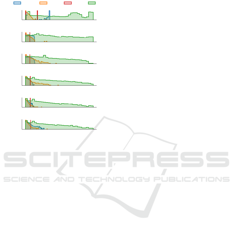
Symmetry Breaking. Figure 10 shows the param-
eter update deviations from the constraints on gradi-
ents induced by translation symmetry, along with the
associated performance after applying the symmetry
breaking regularization.
We see similar trends as for the Leaky ReLU and
batch normalization optimizees. Specifically, L2O
breaks the constraints by a large margin early in the
training run.
ICAART 2024 - 16th International Conference on Agents and Artificial Intelligence
144
0 50
100
Train loss (log scale)
Absolute deviation
Adam
SGD
Lion
L2O, β=0.0
L2O, β=0.1
L2O, β=0.5
0 100 200
Iteration Iteration
0.3
1
2
0
5
10
Figure 10: Symmetry breaking. Left: Translation symme-
try breaking on the optimizee with sigmoid. Right: Perfor-
mance after the translation symmetry breaking regulariza-
tion on the optimizee with sigmoid.
Heavy-Tailedness and Update Covariance. The α
estimates for the gradient and update noise, as well as
the progression of the largest eigenvalue of the update
covariance, are shown in Figures 11 and 12.
Similarly to the results for the Leaky ReLU op-
timizee in the main part of this paper, we can again
observe that L2O dampens the heavy-tailed gradient
noise into high-variation parameter updates. Also, as
mentioned earlier, we observed that the loss during
L2O meta-testing on sigmoid and batch normalization
optimizees starts to increase after around the 500th it-
eration and this accurately correlates with the decreas-
ing α estimates of L2O gradient and update noise we
see here.
Additionally, an interesting observation in itself,
we found that standardizing the image data has a rel-
atively large impact on how heavy-tailed the gradi-
ent and update noise distributions are. Specifically,
when we replaced the data normalization to the range
[0, 1] with standardization, the alpha estimates shifted
around 0.4 lower. Since we tried to follow the setup
from Andrychowicz et al. (2016), all our results were
obtained using data normalization.
0.4
0.6
0.8
1.0
10
-3
10
-2
10
-1
10
0
Adam
SGD
Lion
L2O
0 500
Iteration
1000
0 500
Iteration
1000
Alpha estimate
Adam - updates
Adam - gradients
SGD - updates
SGD - gradients
L2O - updates
L2O - gradients
Largest eigenvalue
Figure 11: Heavy-tailedness and update covariance. Left:
Gradient and update noise on the sigmoid optimizee. Right:
Update covariance on the sigmoid optimizee.
0.4
0.6
0.8
1.0
10
-3
10
-2
10
-1
10
0
Largest eigenvalue
Adam
SGD
Lion
L2O
0 500
Iteration
1000
0 500
Iteration
1000
Alpha estimate
Adam - updates
Adam - gradients
SGD - updates
SGD - gradients
L2O - updates
L2O - gradients
Figure 12: Heavy-tailedness and update covariance. Left:
Gradient and update noise on the optimizee with batch nor-
malization and ReLU. Right: Update covariance on the op-
timizee with batch normalization and ReLU.
Update Histograms. Figures 13 and 14 present his-
tograms of the absolute values of parameter updates
for the optimizee with batch normalization and ReLU
and for the optimizee with Leaky ReLU, respectively.
0.00 0.01 0.02 0.03 0.04 0.05
10
4
10
1
Count
Iteration 1
Adam SGD Lion L2O
0.000 0.025 0.050 0.075 0.100
10
4
10
1
Count
Iteration 5
0.00 0.02 0.04 0.06 0.08
10
4
10
1
Count
Iteration 10
0.00 0.02 0.04 0.06 0.08
10
4
10
1
Count
Iteration 30
0.00 0.02 0.04 0.06 0.08
10
4
10
1
Count
Iteration 100
0.00 0.02 0.04 0.06 0.08
Absolute Value
10
4
10
1
Count
Iteration 500
Figure 13: Histograms of the absolute values of parameter
updates for L2O meta-trained and meta-tested on the opti-
mizee with batch normalization and ReLU.
We can again notice that the learned optimizer
gradually changes the shape of its update distribution
from one in which large values are predominant to a
shape similar to that of Adam.
Investigation into the Training Dynamics of Learned Optimizers
145
0.00 0.01 0.02
10
4
10
1
Count
Iteration 1
Adam SGD Lion L2O
0.00 0.02 0.04 0.06
10
4
10
1
Count
Iteration 5
0.00 0.02 0.04 0.06
10
4
10
1
Count
Iteration 10
0.00 0.02 0.04 0.06
10
4
10
1
Count
Iteration 30
0.00 0.02 0.04 0.06
10
4
10
1
Count
Iteration 100
0.00 0.02 0.04 0.06
Absolute Value
10
4
10
1
Count
Iteration 500
Figure 14: Histograms of the absolute values of parameter
updates for L2O meta-trained and meta-tested on the Leaky
ReLU optimizee.
ICAART 2024 - 16th International Conference on Agents and Artificial Intelligence
146
