Real-Time Deep Learning-Based Malware Detection Using Static and

Dynamic Features

Radu S¸tefan Mihalache, Dragos¸ Teodor Gavrilut¸ and Dan Gabriel Anton

Bitdefender Laboratory, Faculty of Computer Science, ”Al.I. Cuza” University, Ias¸ i, Romania

Keywords:

Malware, Threat Detection, Neural Network, Static Features, Dynamic Features.

Abstract:

Cyber-security industry has been the home of various machine learning approaches meant to be more proac-

tive when it comes to new threats. In time, as security solutions matured, so did the way in which artiﬁcial

intelligence algorithms are being used for speciﬁc contexts. In particular, static and dynamic analysis of a

threat determines certain characteristics of an artiﬁcial intelligence algorithm (such as inference speed, mem-

ory usage) used for threat detection. While from a product point of view, static and dynamic analysis of a

threat target separate product features such as protection for static analysis and detection for dynamic anal-

ysis, the feature sets derived from analyzing threats in those two scenarios (static and dynamic analysis) are

complementary and could improve the accuracy of a model if used together. The current paper focuses on a

multi-layered approach that takes into consideration both static and dynamic analysis of a threat.

1 INTRODUCTION

The cyber-security industry has evolved along with

the constant increase of attacks that led to more than

1.2 billion

known malware in 2023. Nowadays, most

of the cyber-security solutions rely on different ma-

chine learning algorithms for threat detection.

At the same time, cyber-security solutions evolved

in an attempt to cover various needs from both con-

sumer and business markets. One of the major differ-

ences in these cases is that while consumers are more

focused on protection (the role of a security solution

being to make sure that nothing bad happens to a sys-

tem), the business solution also focuses on providing

visibility around an attack. Most of the requirements

that appear in the business market are a direct result of

several compliance rules that enterprises have to obey.

For example, if a cyber-security attack succeeds on a

bank, the bank is required to start an internal inves-

tigation that analyzes logs and additional attack arti-

facts to better understand the impact of that attack.

With this, requirements for a new type of machine

learning algorithm emerge, that focuses on the behav-

ior of an attack and uses logs or asynchronously ob-

tained events to create features that are further used by

the algorithm. These algorithms cannot block a threat

but can provide late triggers about an undergoing at-

https://www.av-test.org/en/statistics/malware/

tack. These triggers are often referred to as detection

capabilities as they do not provide any protection.

Models designs for detection don’t necessarily

need to have a low false positive rate as they can

not block anything. As such they are usually al-

lowed a certain level of false positives if the detection

rate is increased. Another important observation is

that the output of such models is usually analyzed by

a SOC (Security Operation Center) team that deter-

mines if an attack is real or not. This behavior led to a

phenomenon called alert fatigue, meaning that alerts

from these models accumulate to a point where they

are hard to be analyzed by security ofﬁcers.

Our paper focuses on a method that combines two

types of models: based on statically extracted features

and models designed for detection, with the purpose

of reducing the alert fatigue phenomena while pre-

serving a high detection rate. For this purpose we

have used multiple malicious ﬁles that were analyzed

from a dual perspective: a static analysis perspective

where we extract features based on meta information

we can extract from the malicious ﬁles and a dynamic

analysis perspective where we extract features that re-

ﬂect the malware behavior at runtime.

The rest of the paper is organized as follows: sec-

tion 2 reveals similar research, section 3 describes

the current cyber-security landscape and the problem

we are tackling, section 4 presents our approach on

building a neural network that uses both statically and

226

Mihalache, R., Gavrilu¸t, D. and Anton, D.

Real-Time Deep Learning-Based Malware Detection Using Static and Dynamic Features.

DOI: 10.5220/0012316800003636

Paper published under CC license (CC BY-NC-ND 4.0)

In Proceedings of the 16th International Conference on Agents and Artiﬁcial Intelligence (ICAART 2024) - Volume 3, pages 226-234

ISBN: 978-989-758-680-4; ISSN: 2184-433X

dynamically extracted features, section 5 shows the

databases used in our experiment and several results

and ﬁnally, section 6 draws several conclusions on the

practical aspects of our proposal.

2 RELATED WORK

Malware detection has been one ﬁeld that attracted

a lot of attention from researchers who used various

machine learning methods. There are two main ap-

proaches that are usually employed when it comes to

deciding what features will be used in the process of

training and evaluating machine learning models.

The ﬁrst approach involves extracting static fea-

tures from the ﬁles, without executing them. Thus,

this approach usually consumes fewer resources and

reaches high speed and potentially high accuracy.

(Ahmadi et al., 2016) proposed a malware fam-

ily classiﬁcation system, using a wide range of static

features extracted from the original PE executable

ﬁles that were not unpacked or deobfuscated. By

combining the most relevant feature categories and

feeding them to a XGBoost-based classiﬁer, their

model reached an accuracy of around 99.8% on the

Microsoft Malware Challenge dataset (Ronen et al.,

2018) of 20000 malware samples.

Other approaches demonstrated that minimal

knowledge is needed for extracting relevant static

features from executable ﬁles. For instance, a study

demonstrated that effective malware detection can be

obtained using the information in the ﬁrst 300 bytes

from the PE header of executable ﬁles as input (Raff

et al., 2017b). The same year, a more comprehen-

sive study (Raff et al., 2017a) presented MalConv, a

deep convolutional neural network model which di-

rectly uses the raw byte representation of executable

(limited to the ﬁrst 2 MB) as input, without any intelli-

gent identiﬁcation of specialized structures or speciﬁc

executable or malware content. The model showed

good results, achieving 94% accuracy after training

on a large dataset of 2 million PE ﬁles.

In a more recently conducted study (Zhao et al.,

2023), the authors researched a different method, con-

verting the bytecode extracted from the original ﬁles

into color images and using them as input features

for training an AlexNet convolutional neural network

(CNN). The results were promising, the accuracy of

their model reaching more than 99% on two rather

small public malware datasets from Google Code Jam

and Microsoft of around 10000 samples.

However, using static features alone might bring

some limitations in real-world malware detection sce-

narios where advanced obfuscation, packing or en-

cryption are being used for creating malicious ﬁles.

In a recent study (Aghakhani et al., 2020) this aspect

was investigated and, using a dataset of almost 400

thousand ﬁles, it was demonstrated that using static

information exclusively is not indicative of the actual

behavior of the classiﬁed ﬁles and a substantial num-

ber of false positives on packed benign ﬁles occur.

The other main approach would be to extract dy-

namic features that describe the behavior of the mal-

ware during execution or partially retain information

regarding the said behavior.

One method is to include dynamic runtime op-

codes as input features, allowing the behavior of ex-

ecutables to be captured. An extensive study (Carlin

et al., 2019) showed that this approach can accurately

detect malware, even on a continuously growing and

updatable dataset that requires retraining. The authors

compared 23 machine learning algorithms and con-

cluded that their method worked best using the Ran-

dom Forest model.

In a recent study (Zhang et al., 2023), the authors

proposed another method of combining the API call

sequences-based dynamic features with the semantic

information of functions, bringing more context to the

actual performed action by the API call. Compared

to existing similar experiments that only used API

call information, their solution shows improvements

of 3% to 5% in detection accuracy.

(Ijaz et al., 2019) compare several methods based

on machine learning for detecting Windows OS ex-

ecutables. They use a small set of ﬁles of only

39000 malicious binaries and 10000 benign ones,

from which they statically extract a small set of 92

features from the PE headers using the PEFILE tool.

They also dynamically extract 2300 features from a

small part of the ﬁles from the execution in Cuckoo

Sandbox. Their detection measurements are made us-

ing either the static features or the dynamic features

separately. Also, using a sandbox for the training

and evaluation part when using the dynamic features

brings in a series of disadvantages, because it does

not provide a form of real-time protection for the new

malicious ﬁles that would need to be evaluated.

In one of the ﬁrst such approaches, (Santos et al.,

2013) present a hybrid malware detection system that

combines both static and dynamic features. The

small dataset they use consists of 1000 malware and

1000 legitimate ﬁles, from which they extract two-

byte opcodes, perform feature selection using Infor-

mation Gain and select the ﬁrst 1000 as the static fea-

tures that will be used. The dynamic characteristics

are extracted by monitoring the behavior of the pro-

grams in a controlled sandboxed environment.

Another different hybrid approach that uses both

Real-Time Deep Learning-Based Malware Detection Using Static and Dynamic Features

227

static and dynamic features for malware detection is

proposed in (Zhou, 2019). The authors use a sandbox

for recording API call sequences from the execution

of 90000 malicious and benign ﬁles and they extract

dynamic features out of a trained RNN model that is

fed with the recorded sequences. The static and dy-

namic features are then combined into custom images

that will be used in the training and validation phase

of a CNN model. Both studies demonstrate how com-

bining both static and dynamic characteristics brings

improvements in detection rates.

Compared to our approach, these two studies have

a few limitations, one related to the small number of

ﬁles used in the dataset and another related to the us-

age of a sandbox for extracting dynamic features dur-

ing execution. Thus, their systems could provide only

ofﬂine detection and classiﬁcation mechanisms and

are no practical solutions for a product which must

provide real-time protection against malware.

3 PROBLEM/SECURITY

LANDSCAPE

The cat-and-mouse game has been a constant of the

cyber-security ecosystem for decades; malicious ac-

tors create a new threat, cyber-security solutions adapt

then the new threats adapt to the new cyber-security

changes and the cycle goes on. And while this type of

change is inevitable, there were other (more business-

related) changes that a security product suffered dur-

ing the years.

One such important change was the split between

types of users: enterprise and consumer. While con-

sumer users are more interested in protection (the

security solution is perceived as a tool that quietly

ensures that everything is secured), the business en-

vironment comes with several different challenges.

When a breach happens, there is a need (sometimes

driven by compliance regulations) to understand ex-

actly what endpoints were affected, what kind of data

was exﬁltrated, when the attack started or what set of

measures would reduce the chance for a similar attack

to happen in the future.

While these differences relate mostly to a prod-

uct feature (centralized dashboard, reports for en-

terprise environment and automated ﬂows for con-

sumer), there are several differences that regard threat

detection as well. As a result, threat detection differ-

ences can be classiﬁed in regards to:

• Static Detection - usually associated with pre-

execution / on-access scanners. The main char-

acteristic of this type of detection is that it takes

a ﬁle as an input (but a ﬁle that was not executed

yet) and analyzes it (in terms of its content). Se-

curity products refer to this type of detection as

protection as that ﬁle is not executed yet and de-

tecting it at this point blocks the attack and keeps

the user protected. This is heavily used in con-

sumer products where the expectation is to block

everything and keep the user protected.

• Dynamic Detection - usually associated with

post-execution scanners. It implies that the ﬁle

is allowed to run, while at the same time its ac-

tions are monitored. This type of detection is bet-

ter at identifying behavior and intent, but it’s less

resilient in terms of protection (once some data is

copied to an external site, even if we record the

event, we cannot un-copy it). Enterprise solutions

use this method as part of EDR/XDR products to

record data related to an attack and automatically

create a root cause report.

From a detection point of view (and in particular,

if we refer to machine learning models) there are sev-

eral distinct features that each of these two detection

methods (static and dynamic) have:

• Static Detection methods are usually used in the

pre-execution phase. This actually means that for

example, before a ﬁle gets executed, its content

is scanned. From a technical perspective, this is

achieved via a kernel mode driver that stops the

execution until the result from the scanner is avail-

able. While this method ensures protection (noth-

ing gets executed unless it was scanned), it also

imposes certain limitations. If for example, the

duration of a scan is one second for each ﬁle,

the entire operating system will be heavily slowed

down. As such, models that are used in this phase

have to be fast (fewer neurons or other forms

of more classical machine learning approaches

such as binary decision trees, random forests, etc).

It’s also important to notice that features used in

these methods are extracted directly from the ﬁle

content (strings, section information, disassembly

listings, imports and exports, etc) and don’t reﬂect

the behavior of a sample but rather a probability of

something being malicious.

• Dynamic Detection on the other hand is used

with events that are recorded asynchronously. As

such, the performance impact is reduced and as-

suming storage space is not an issue, larger mod-

els (e.g. neural networks with multiple hidden

layers) can be used. It is also worth mentioning

that the input to these models reﬂects behavior

(system events, APIs that are being used, etc).

As a general concept, a security solution uses

these two forms of detection sequentially (ﬁrst a ﬁle

ICAART 2024 - 16th International Conference on Agents and Artiﬁcial Intelligence

228

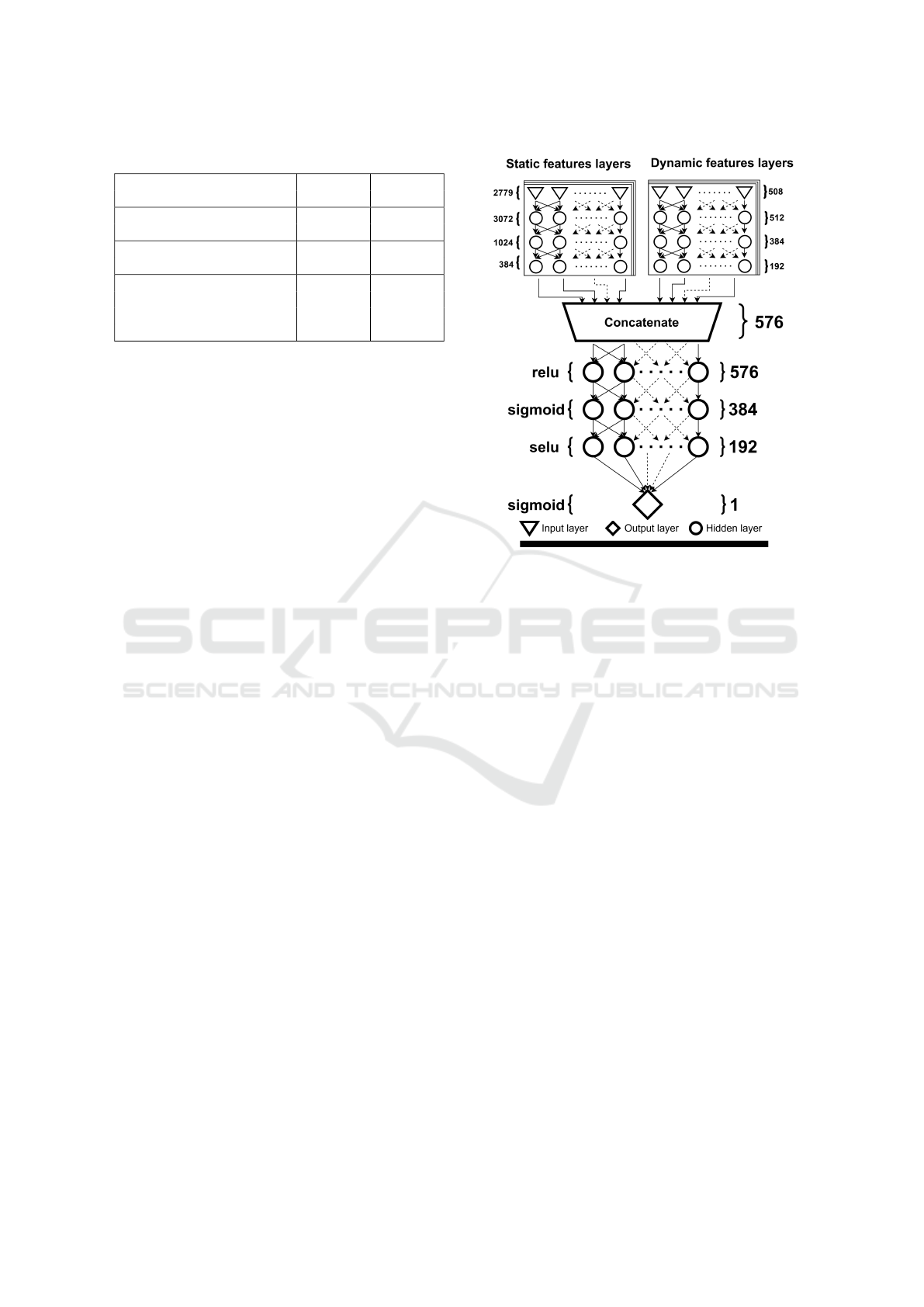
Table 1: Static vs dynamic detection.

Static Dynamic

Detection Detection

Susceptible to packers and Yes No

obfuscation techniques

Behavior false positive No Yes

(use of startup registry keys)

Susceptible to dynamic No Yes

detection evasion techniques

(behave differently if

monitored)

is scanned with the static scanner, then if nothing is

found it gets executed and the dynamic scanner ana-

lyzes it). However, each one of these two solutions

comes with several limitations in terms of detection -

as shown in table 1.

Since these evasion techniques are often used by

advanced malware in different stages of an attack, us-

ing just one of these detection methods or both but

sequentially may be ineffective.

4 SOLUTION

In order to address the problem of advanced malware

detection, we set on developing a neural network that

classiﬁes a program as benign (labeled 0) or mali-

cious (labeled 1) by analyzing static features of the

program’s ﬁle as well as dynamic features of the pro-

cess runtime behavior. Our solution targets PE ﬁles.

We chose to use deep learning because it allowed

us to apply transfer learning and also because it pro-

vided better results than other modeling approaches

(described in section 5.2).

To aid this approach, we designed the neural net-

work with two branches that process static and dy-

namic features separately. Results from these two

branches are concatenated and then fed to layers re-

sponsible for correlating static with dynamic data.

The diagram in ﬁgure 1 displays this architecture.

There are 2779 static features and 508 dynamic

features. These are fed through separate branches of

the neural network. A total of 576 values result by

concatenating the outputs of the static and dynamic

feature branches. These 576 values are fed through

fully connected layers of decreasing sizes (576, 384,

192). These were chosen by experimenting with neu-

ral layer sizes that are multiples of powers of 2.

In order to address the dying ReLU problem, we

experimented with SELU activation. On some layers,

this activation function improved the model’s perfor-

mance. SELU is a variant of ReLU that makes possi-

ble to compute non-zero gradients on negative values.

Figure 1: Proposed solution.

By having different sections of the neural network

that process static and dynamic features, we are able

to train neurons in these two sections separately. This

makes it possible to overcome a situation where for

training purposes, there is a lack of dynamic data but

an abundance of static data (as we will show later on,

this is the case).

An important point to make is that our solution

could perform well even against ﬁleless malware.

Fileless malware infects legitimate programs already

present on the endpoint. Our solution could ascertain

the expected behavior of a legitimate program based

on the static analysis of the executable ﬁle and com-

pare it with the actual runtime behavior. Thus, if un-

expected suspicious actions occur that are indicative

of a ﬁleless malware attack, a detection may be raised

with greater accuracy.

4.1 Static Component

The branch that analyzes static features is made up

of the ﬁrst 4 layers of the neural network displayed

in ﬁgure 2. This neural network was trained as a self-

contained model and used to initialize weights and bi-

ases in the static feature branch of the ﬁnal model.

The neural network in ﬁgure 2 takes as input static

features of a PE ﬁle. These features consist of both

boolean and numeric values. In order to extract static

features we used an AntiMalware engine that ana-

lyzes the structure and contents of the ﬁle.

Real-Time Deep Learning-Based Malware Detection Using Static and Dynamic Features

229

Figure 2: Layers for static features.

Examples of static features that were utilized are

found in table 2. Some of the features listed below

may be represented as ﬁxed-length collections of nu-

meric or boolean values (for example, the APIs his-

togram).

Table 2: Examples of static features.

File header characteristics

Byte histogram

Used APIs histogram

Speciﬁc library imports

Byte patterns speciﬁc to known behavior (for exam-

ple, decoding memory section with XOR)

Known packer type used by ﬁle

4.2 Dynamic Component

Similar to the static component, the branch that ana-

lyzes dynamic features is made up of the ﬁrst 4 layers

of the neural network displayed in ﬁgure 3. This neu-

ral network was trained as a self-contained model and

then used to initialize weights and biases in the dy-

namic feature branch of the ﬁnal model.

The neural network in ﬁgure 3 takes input dy-

namic features extracted based on the process behav-

ior at runtime. In order to obtain these features we

used an EDR security solution (Endpoint Detection

and Response) which is installed on the machine and

it extracts dynamic features in real-time by monitor-

ing the process at runtime and the entire system at

large. The EDR solution correlates a sequence of

events representing actions done by the process. Mul-

tiple sensors installed on the machine monitor opera-

tions and send events to the correlation component.

Some of the used sensors are API hooks, network

probes and Event Tracing for Windows.

Examples of examined events and the correlation

logic used for extracting dynamic features are found

in table 3. The resulting dynamic features consist of

both boolean and numeric values.

Figure 3: Layers for dynamic features.

Table 3: Examples of runtime events and dynamic features.

Event name Example of dynamic feature

Process create

A process with suspicious com-

mand line arguments was created

Process inject

Code was injected into a running

process

Process load

module

A suspicious module was loaded

through DLL Search Order Hi-

jacking

Process API

call

A process called an asymmetric

encryption API

Windows

Management

Instrumenta-

tion operation

A process performed a suspi-

cious operation through Win-

dows Management Instrumenta-

tion

Registry

value write

A value was written in a registry

startup key

Network con-

nect

A process made an HTTP con-

nection to an untrusted domain

File create

A ﬁle was created that has a

name speciﬁc to a ransomware

note

File delete

Multiple user ﬁles were deleted -

possible destruction of data

4.3 Evaluation Triggers

The proposed neural network is meant to be integrated

into an EDR security product where performance im-

pact is of the essence. This requires an efﬁcient eval-

uation mechanism for the neural network.

Dynamic features are extracted as the program

is running. The evaluation mechanism must decide

when to perform a neural network inference in order

to detect a malware program as early in its execution

as possible. In order not to affect performance, infer-

ence should be performed only a limited number of

times per period and only when it is relevant.

The diagram in ﬁgure 4 displays the evaluation

mechanism we have chosen for EXE ﬁles. The mech-

anism for DLL ﬁles is similar but evaluation starts af-

ICAART 2024 - 16th International Conference on Agents and Artiﬁcial Intelligence

230

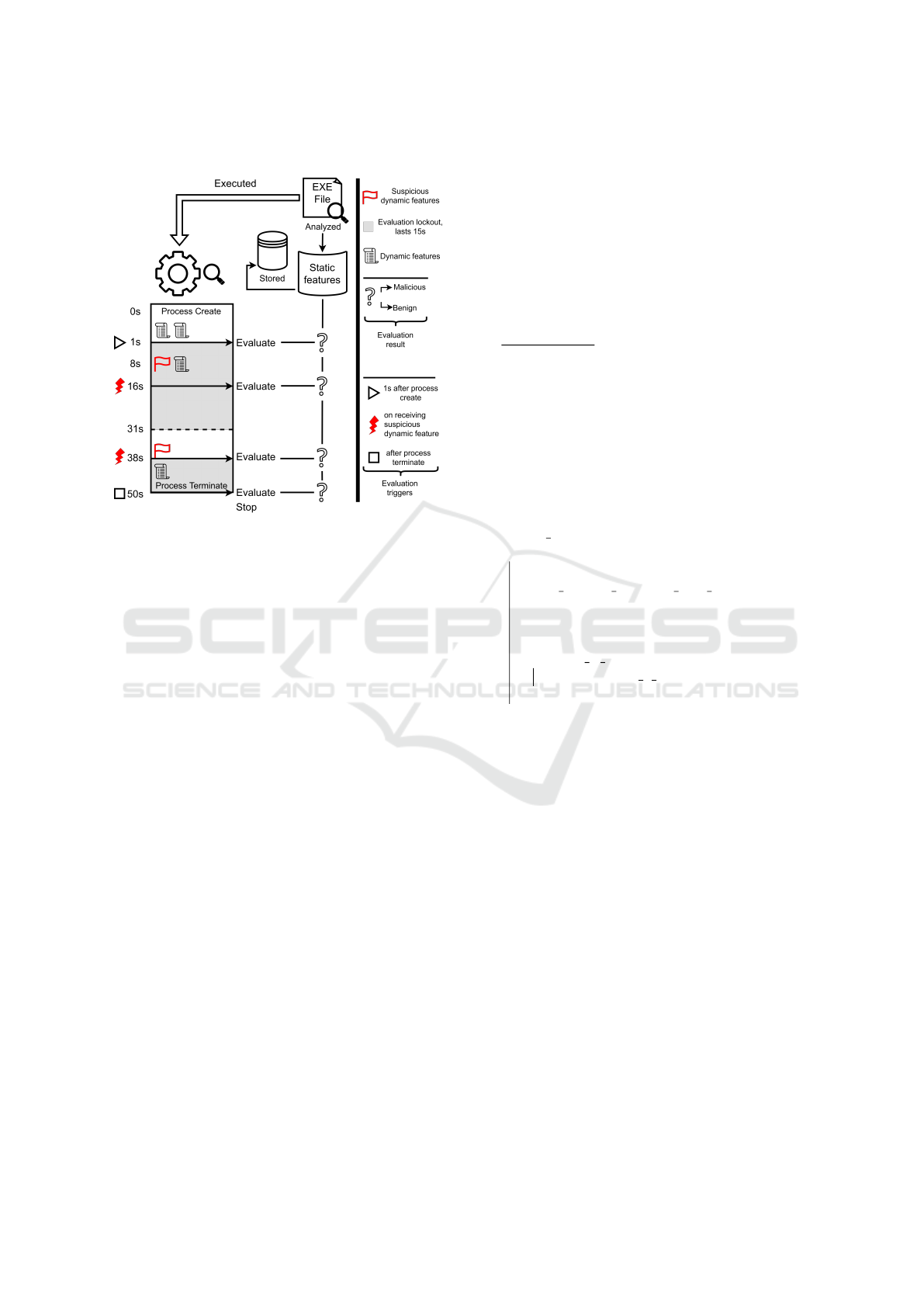
ter a process has loaded the DLL module.

Figure 4: Evaluation triggers and steps.

As shown above, for evaluation to be triggered,

static features of the EXE ﬁle must be available and a

process needs to have started execution based on said

EXE ﬁle. If those conditions are met, evaluation is

triggered in the following cases: one second into the

process execution, when a suspicious dynamic feature

is received and after the process is terminated.

After each time an evaluation is performed, an

evaluation lockout period is put in place for said pro-

cess in order to prevent a ﬂood scenario that would

impact performance. The evaluation lockout period

lasts 15 seconds.

The evaluation triggers and overall logic is similar

for DLL ﬁle analysis.

5 RESULTS

5.1 Database

We used a private dataset containing 5455942 PE

ﬁles, of those 4068535 are labeled benign and

1387407 are labeled malicious. The reason for the

dataset containing 75% benign ﬁles is to reﬂect that

on a typical computer, there are many more benign

ﬁles than malicious ones. As such, this ratio helps us

avoid a model prone to false positive alerts.

The static features representing the PE ﬁle struc-

ture were extracted using a component of an AntiMal-

ware solution. Examples of static features are found

in table 2.

There were more than 150000 static features ex-

tracted for each ﬁle. Much like in (Dahl et al., 2013)

we had to reduce the number of features that would

be used for the model based on static features. The

total uncompressed size of the static data was 5.5TB.

In order to perform feature selection on such a large

quantity of data in a reasonable amount of time we

had to do the selection in multiple steps. These con-

secutive steps are described by the function Select.

function Select (D,limit,S,c);

Input : D dataset

limit the maximum amount of data

able to be processed

S selection methods

c maximum length of set A

containing relevant features

Output: Set A with the most relevant

features

A = all f eatures(D);

largest n s.t. n ∗ len(A) < limit;

d = n random instances with features(D,

n, A);

k = max(c, len(A)/2);

A = {};

for select

K best in S do

A = A ∪ select k best(d, k);

end

while len(A) > c;

Algorithm 1: Progressively select the best features of

the dataset.

The methods that we used for selecting the best

static features are the maximum information gain and

the importance given by a random forest classiﬁer

trained on the dataset.

While there are many sandbox tools that emu-

late the execution of a PE ﬁle, nowadays there are

malware programs that employ anti-emulation tech-

niques. Considering that, we decided to run the ﬁles

on virtual machines with an EDR sensor installed.

The execution of the ﬁle produces a sequence of

events that are correlated by the EDR sensor through

various heuristics. These heuristics provide behavior

ﬂags representing the dynamic features of a ﬁle’s exe-

cution. Examples of events and dynamic features ex-

tracted by the EDR sensor are found in table 3.

To minimize the time required for extracting dy-

namic features, we developed a system that uses mul-

tiple virtual machines to run PE ﬁles in parallel.

As displayed in ﬁgure 5, each ﬁle is run on a vir-

Real-Time Deep Learning-Based Malware Detection Using Static and Dynamic Features

231

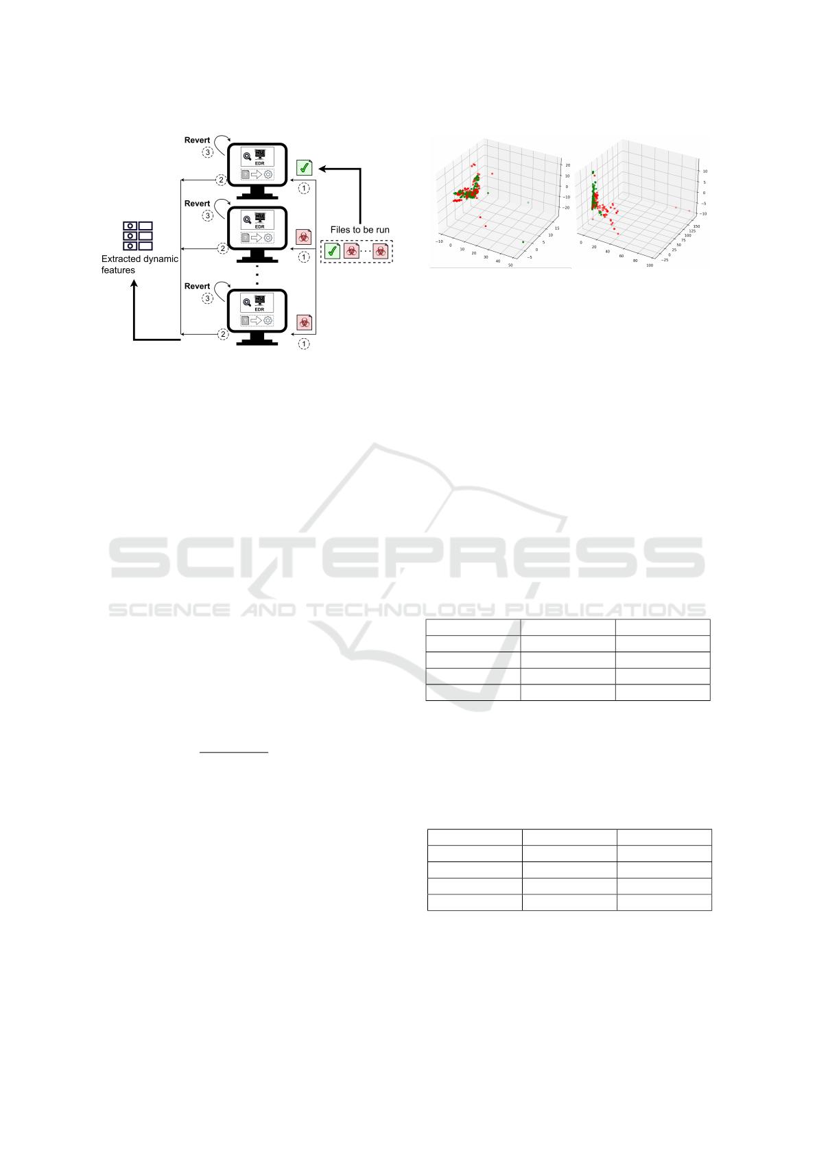
Figure 5: Sample running and dynamic feature extraction

system.

tual machine for at most 3 minutes, the EDR sensor

extracts dynamic features, then the virtual machine is

reverted to an earlier snapshot in order to mitigate any

damage done by a malware program. Even with 10

virtual machines running samples in parallel, it would

have taken more than 3 years to extract dynamic fea-

tures for all ﬁles. Because of that, we selected in

a random uniform manner 13814 ﬁles. For 13217

of those we were able to extract dynamic features,

9978 labeled benign and 3239 labeled malicious, thus

maintaining the original ratio.

To clean up the dataset, we performed an analysis

on samples with static and dynamic data.

C - set of samples correctly classiﬁed by either the

model using static features or the model using dy-

namic features

M - set of samples incorrectly classiﬁed by both the

model using static features and the model using dy-

namic features

m,K

- set of the K closest neighbors of m from C

based on Hamming Distance

∆

(m) =

∑

n∈N

m,K

(m,n) + ε



γ, y

= y

1 − γ, y

̸= y

m ∈ M; d

- Hamming Distance; γ = 0.85

- label of m; y

- label of n

We chose γ = 0.85 to minimize the chances of re-

moving a correctly labeled sample from the dataset.

Based on these statistics, we removed 212 samples

we found to be possible mislabels. This represents

1.6% of the dataset containing dynamic features and

0.00003% of the dataset containing static features.

In order to visualize the extracted data, we per-

formed a PCA analysis. Figure 6 displays the PCA

analysis for static (left side) and dynamic (right side)

data.

Figure 6: Static data PCA and Dynamic data PCA.

5.2 Training & Inference

The training process was performed separately for the

model that uses static features and the model that uses

dynamic features. These two neural networks serve

as the building blocks to the ﬁnal model that makes

use of transfer learning to better correlate static and

dynamic features.

In order to obtain the best results, the values of

both static and dynamic features in datasets were nor-

malized such that the standard deviation σ = 1 and the

mean µ = 0.

The neural network for static features was trained

for 30 epochs with a variable learning rate starting

from lr = 0.001 and then decreasing from epoch 5

by lr = lr · e

−0.16

. The loss function used was binary

cross entropy. To measure the model’s performance

we used K-fold cross-validation with 5 folds.

Table 4: Performance of the model using static features.

Metric Value STD Dev

FP Rate 0.368% 0.00086

TP Rate 86.746% 0.00195

F1 Score 92.234% 0.00022

Accuracy 96.346% 0.00016

The neural network using dynamic features was

trained on 30 epochs with a variable learning rate sim-

ilar to the model using static features and binary cross

entropy loss function. Its performance was measured

using K-fold cross-validation with 5 folds.

Table 5: Performance of the model using dynamic features.

Metric Value STD Dev

FP Rate 0.716% 0.00155

TP Rate 81.52% 0.01331

F1 Score 88.52% 0.00940

Accuracy 94.832% 0.00476

We wanted to see if we could obtain better per-

formance by training other machine learning algo-

rithms on the dynamic features. We tested the accu-

racy of both Random forest and XGBoost with 100

ICAART 2024 - 16th International Conference on Agents and Artiﬁcial Intelligence

232

estimators against our result obtained with a neural

network. As it turns out, Random forest algorithm

obtained 93.171% and XGBoost 93.394%, both less

than 94.832% that was obtained by our neural net-

work.

The ﬁnal neural network uses both static and dy-

namic features and it processes them on two different

branches. Neurons on these branches load weights

and biases from the previous two models that are al-

ready trained, thus making use of transfer learning. At

ﬁrst, only neurons processing the concatenated results

from the ﬁrst two branches are trained, but after a cer-

tain epoch and learning rate, all neurons are trained.

We used this scheme in order to make the model

learn based on knowledge already gained by the pre-

vious two models. In this way, we are able to take full

advantage of the large number of instances with static

data while also using the statistically representative

number of instances with dynamic data. Furthermore,

by using this training scheme we were able to reduce

overﬁtting and obtain a considerable performance im-

provement.

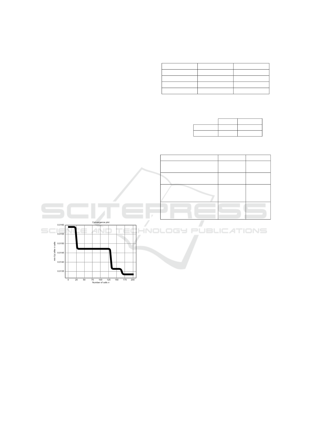
In order to ﬁnd the best combination of hyper-

parameters, we used a Bayes search algorithm that

tries to minimize a function we chose f (model) =

1 − F1Score(model). Figure 7 displays the value of

this function at the number of attempts made by the

Bayes search algorithm.

Figure 7: Bayes search graphic.

The neural network that uses both static and dy-

namic features was trained on 25 epochs with a vari-

able learning rate that decreases starting from epoch

10. When epoch > 21 and lr < 0.00025 all layers of

the network are trained. The loss function used was

binary cross entropy. To measure the model’s perfor-

mance we used K-fold cross-validation with 5 folds.

In order to thoroughly analyze the performance

of the model that uses static and dynamic features,

we also considered the Confusion Matrix for thresh-

old=0.5 and the ROC AUC. The total ROC Area Un-

der the Curve is 0.99896.

Table 6: Performance of the model using static and dynamic

features.

Metric Value STD Dev

FP Rate 0.26% 0.00147

TP Rate 97.822% 0.00326

F1 Score 98.47% 0.00389

Accuracy 99.302% 0.00143

Table 7: Confusion Matrix of the model using static and

dynamic features.

Predicted

Clean Malware

Ground truth

Clean 10532 34

Malware 60 3188

Table 8: Analysis of correctly classiﬁed samples by com-

bined model.

Element Accuracy

Correctly classiﬁed by

analyzing static data

S ∩C 98.704%

Improvement by analyz-

ing dynamic data

(D \S) ∩C 0.6%

Improvement by correlat-

ing both static and dy-

namic data

C \(S ∪D) 0.0144%

Total correctly classiﬁed

samples by combined

model

C 99.319%

6 CONCLUSIONS

Based on the results, we can conﬁdently say that the

model using combined features is best suited for prac-

tical application. By having the highest TP rate and

the lowest FP rate, the combined model is able to

raise alerts that offer a high degree of visibility while

keeping alert fatigue at a minimum. This offers a way

for cyber-security analysts to quickly identify an ad-

vanced threat without having to shift through large

amounts of false positive alerts.

Taking a closer look, we found that the increase in

accuracy was not just comprised of samples correctly

identiﬁed by either the model using just static fea-

tures or the model using dynamic features. The model

using combined features correctly classiﬁed samples

that neither of the two previous models did. This pro-

vides a way to counteract advanced attacks better.

We tested each model on the dataset containing

both static and dynamic features.

Let S, D, and C be the sets of samples correctly

labeled by each model (S for the model using static

data, D for the model using dynamic data and C for

Real-Time Deep Learning-Based Malware Detection Using Static and Dynamic Features

233

Figure 8: ROC AUC of the model using static and dynamic

features.

the model using combined data).

In table 8 we show how using static and dynamic data

contributes to the ﬁnal model performance. Keep in

mind that, as accuracy approaches 100%, even small

improvements are signiﬁcant, especially in the ﬁeld

of malware detection.

One disadvantage our solution currently has is that

it was trained using just the initial access stage of an

attack. While from a protection perspective, this is

desired, the EDR philosophy is to provide visibility.

In the next iteration, we plan to train the model using

events from multiple steps of an attack, from initial

access to exﬁltration.

REFERENCES

Aghakhani, H., Gritti, F., Mecca, F., Lindorfer, M., Or-

tolani, S., Balzarotti, D., Vigna, G., and Kruegel, C.

(2020). When malware is packin’ heat; limits of ma-

chine learning classiﬁers based on static analysis fea-

tures. Proceedings 2020 Network and Distributed Sys-

tem Security Symposium.

Ahmadi, M., Ulyanov, D., Semenov, S., Troﬁmov, M., and

Giacinto, G. (2016). Novel feature extraction, selec-

tion and fusion for effective malware family classiﬁ-

cation.

Carlin, D., Okane, P., and Sezer, S. (2019). A cost analysis

of machine learning using dynamic runtime opcodes

for malware detection. Computers & Security, 85.

Dahl, G. E., Stokes, J. W., Deng, L., and Yu, D. (2013).

Large-scale malware classiﬁcation using random pro-

jections and neural networks. In 2013 IEEE Inter-

national Conference on Acoustics, Speech and Signal

Processing, pages 3422–3426.

Ijaz, M., Durad, M. H., and Ismail, M. (2019). Static and

dynamic malware analysis using machine learning. In

2019 16th International Bhurban Conference on Ap-

plied Sciences and Technology (IBCAST), pages 687–

691.

Raff, E., Barker, J., Sylvester, J., Brandon, R., Catanzaro,

B., and Nicholas, C. K. (2017a). Malware detection

by eating a whole exe. In AAAI Workshops.

Raff, E., Sylvester, J., and Nicholas, C. (2017b). Learn-

ing the pe header, malware detection with minimal do-

main knowledge. pages 121–132.

Ronen, R., Radu, M., Feuerstein, C., Yom-Tov, E., and Ah-

madi, M. (2018). Microsoft malware classiﬁcation

challenge. CoRR, abs/1802.10135.

Santos, I., Devesa, J., Brezo, F., Nieves, J., and Bringas,

P. G. (2013). Opem: A static-dynamic approach

for machine-learning-based malware detection. In

Herrero,

A., Sn

sel, V., Abraham, A., Zelinka, I.,

Baruque, B., Quinti

an, H., Calvo, J. L., Sedano, J.,

and Corchado, E., editors, International Joint Confer-

ence CISIS’12-ICEUTE 12-SOCO 12 Special Ses-

sions, pages 271–280, Berlin, Heidelberg. Springer

Berlin Heidelberg.

Zhang, S., Wu, J., Zhang, M., and Yang, W. (2023). Dy-

namic malware analysis based on api sequence seman-

tic fusion. Applied Sciences, 13:6526.

Zhao, Z., Zhao, D., Yang, S., and Xu, L. (2023). Image-

based malware classiﬁcation method with the alexnet

convolutional neural network model. Security and

Communication Networks, 2023:1–15.

Zhou, H. (2019). Malware detection with neural network

using combined features. In Yun, X., Wen, W., Lang,

B., Yan, H., Ding, L., Li, J., and Zhou, Y., editors, Cy-

ber Security, pages 96–106, Singapore. Springer Sin-

gapore.

ICAART 2024 - 16th International Conference on Agents and Artiﬁcial Intelligence

234