Metrics for Popularity Bias in Dynamic Recommender Systems

Valentijn Braun

, Debarati Bhaumik

and Diptish Dey

Amsterdam University of Applied Sciences, Netherlands

Keywords: Recommender Systems, Popularity Bias, Fairness, Dynamic.

Abstract: Albeit the widespread application of recommender systems (RecSys) in our daily lives, rather limited research

has been done on quantifying unfairness and biases present in such systems. Prior work largely focuses on

determining whether a RecSys is discriminating or not but does not compute the amount of bias present in

these systems. Biased recommendations may lead to decisions that can potentially have adverse effects on

individuals, sensitive user groups, and society. Hence, it is important to quantify these biases for fair and safe

commercial applications of these systems. This paper focuses on quantifying popularity bias that stems

directly from the output of RecSys models, leading to over recommendation of popular items that are likely

to be misaligned with user preferences. Four metrics to quantify popularity bias in RescSys over time in

dynamic setting across different sensitive user groups have been proposed. These metrics have been

demonstrated for four collaborative filtering based RecSys algorithms trained on two commonly used

benchmark datasets in the literature. Results obtained show that the metrics proposed provide a

comprehensive understanding of growing disparities in treatment between sensitive groups over time when

used conjointly.

1 INTRODUCTION

RecSys have become an integral part of our daily

lives, influencing the products we buy, the movies we

watch, the music we listen to, so on and so forth (Lu

et al., 2015). These systems aim to predict users'

preferences and provide personalized

recommendations by analysing their past behaviour,

preferences, and interactions (Lü et al., 2012). The

explosion of e-commerce and the growth of online

platforms resulted in RecSys becoming essential tools

for businesses to increase user engagement and

customer loyalty (Khanal et al., 2020). Similarly,

RecSys are also finding its applications in sensitive

sectors such as law enforcement (Oswald et al.,

2018), health care (Schäfer et al., 2017), and human

resources (Vogiatzis & Kyriakidou, 2021); usage in

these sensitive sectors necessitates that

recommendations provided can be explained,

evaluated, and demonstrably unbiased & fair.

Contemporary research in RecSys has focussed

on improving accuracy and processing speed (Chen

https://orcid.org/0009-0009-5441-4528

https://orcid.org/0000-0002-5457-6481

https://orcid.org/0000-0003-3913-2185

et al., 2023). Meanwhile, RecSys algorithms continue

to be trained on data with real-world user behaviour,

which is shown to contain various biases such as

representation bias and measurement bias (Mehrabi et

al., 2021), despite that research on biases in RecSys

lacks consensus on definition of bias (Chen et al.,

2023; Deldjoo et al., 2023). Additionally, prior works

on algorithmic fairness focus primarily on defining

conditions for fairness to answer the question “is an

algorithm unfair?”, but do not provide evaluation

metrics for unfairness to answer how unfair an

algorithm is (Speicher et al. (2018)). This is further

supported by Lin et al. (2022), emphasising on how

to quantify bias in RecSys still remains understudied.

Bias, in context of RecSys, can be viewed as

recommendations provided by such systems that may

potentially lead to discrimination towards certain

items, groups or individuals based on factors such as

demographics, item popularity, personal preferences

or historical data (Chen et al., 2021). The various

types of biases that exist in RecSys can be categorized

into four categories: data bias, model bias, results

Braun, V., Bhaumik, D. and Dey, D.

Metrics for Popularity Bias in Dynamic Recommender Systems.

DOI: 10.5220/0012316700003636

Paper published under CC license (CC BY-NC-ND 4.0)

In Proceedings of the 16th International Conference on Agents and Artiﬁcial Intelligence (ICAART 2024) - Volume 2, pages 121-134

ISBN: 978-989-758-680-4; ISSN: 2184-433X

121

bias, and amplifying biases (Chen et al., 2023).

Data bias refers to biases that are present in input

data used to train RecSys algorithms. This consists of

selection bias, conformity bias, exposure bias, and

position bias. Selection bias arises from users’

freedom to choose which items to rate, leading to

users tending to select and rate items that they like

and are more likely to rate particularly good or bad

items (Marlin et al., 2007). Conformity bias involves

users rating items in line with group behaviour and

not to their true preferences (Liu et al., 2016).

Exposure bias results from disproportionate

presentation of unpopular items to users compared to

popular items (Liu et al., 2020), whereas position bias

occurs when item positions in a list of recommended

items influence user interaction (Collins et al., 2018).

Model bias represents inductive biases that are

purposefully added to the model design in order to

achieve desirable results which cannot be derived

from training data (Chen et al., 2023).

Results bias pertains to biases that originate

directly from output of RecSys models. Such biased

recommendations lead to: (i) popularity bias, where

popular items are recommended with higher

propensity, potentially mismatching user preferences,

and (ii) unfairness, in which discriminatory

recommendations are provided to certain individuals

or groups with specific attributes like race or gender

(Mehrabi et al., 2021; Ekstrand et al., 2018).

Amplifying biases occur when existing biases

present in the data, model or results are amplified

unintentionally, thus, intensifying disparities. This

effect involves self-reinforcing feedback loops where

recommendations reinforce existing preferences and

perpetuate bias (Mansoury et al., 2020).

Biased recommendations have varied negative

consequences (Kordzadeh & Ghasemaghaei, 2022);

Popularity bias might undermine user’s interactions

with items that are unpopular and prevent them from

becoming popular (Baeza-Yates, 2020). Mehrotra et

al. (2018) illustrated that a small number of popular

artists on Spotify get an overwhelmingly larger

number of listens, resulting in an unfavourable

consequence for the remaining less renowned

musicians. Similarly, it has been studied that

popularity and demographic biases led to users with

different ages, genders, and/or demographics

receiving recommendations with significant

differences in accuracy (Ekstrand et al., 2018). Since,

these factors can potentially lead to discrimination

and unfairness towards individuals or groups, it is

important to quantify popularity bias and unfairness

in RecSys (Deldjoo et al., 2023; Ekstrand et al., 2018;

Mehrabi et al., 2021).

Studies done on quantifying popularity bias

mostly focus either on static settings or at a global

level (Ahanger et al., 2022; Abdollahpouri et al.,

2019; Ekstrand et al., 2018). However, in real-life

applications, unfairness may only become apparent

over time across different user groups. To measure

unfairness, this paper proposes metrics to quantify

popularity bias in dynamic settings across sensitive

user groups in RecSys.

In section 2, metrics currently used to measure

popularity bias and their limitations are discussed. In

section 3, the proposed metrics for quantifying

popularity bias over time across various sensitive user

groups are presented. In section 4 the proposed

metrics are demonstrated using two commonly used

datasets in literature for two sensitive user groups,

males and females. In section 5 and 6, conclusions

and future work are discussed, respectively.

2 POPULARITY BIAS IN RECSYS

When training algorithms on long-tailed data, RecSys

models tend to give higher scores to items that are

more popular, resulting in popular items being

recommended with higher propensity than their

actual popularity (Abdollahpouri & Mansoury,

2020). This results in recommendations provide by a

RecSys based on a biased selection of items that do

not align with the user's actual preferences, thereby,

negatively impacting the user experience (Bhadani,

2021). Additionally, if popularity bias is ignored, a

negative feedback loop can result in popular items

getting even more popular (Zhu et al., 2021).

It is important to note that popularity bias is not

always harmful. Item popularity is not only a result of

conformity, where people tend to behave similarly to

others within a group but can also result from the item

being of high quality. This implies that leveraging

popularity bias appropriately into a RecSys may

improve its performance (Zhao et al., 2022).

2.1 Static versus Dynamic Setting

Studies conducted on evaluating fairness in RecSys

use either a static or dynamic setting. Whereas static

refers to data usage at a single point of time, dynamic

setting includes usage of user interaction data over

time including feedback interactions; the latter being

closer to real-life implementations. Access to real-life

dynamic data is a challenge. As a result,

approximately 85% percent of recent studies on

RecSys are performed on static data (Deldjoo et al.,

2023). Evaluating biases in RecSys within static

ICAART 2024 - 16th International Conference on Agents and Artiﬁcial Intelligence

122

settings may lead to under-representation of

unfairness as it may only surface over time.

To this end, to measure biases in RecSys without

access to real dynamic data from live platforms, user

interactions must be simulated from static datasets. A

common approach to transform a static dataset into a

dynamic one by simulating new (dynamic)

interactions (Aridor et al., 2020; Chong & Abeliuk,

2019; Zhu et al., 2021; Khenissi et al., 2020) is

deployed in this paper. This approach uses the

assumption that users interact with their top-N

recommendations and appends these interactions to

the static dataset for a predefined number of

iterations. An iteration is a step in which a RecSys

algorithm is trained to provide top-N

recommendations to each user and their interaction is

simulated (see section 4.2).

2.2 Individual versus Group Fairness

Concepts in algorithmic fairness can be categorized

into two groups: individual- and group- fairness

(Dwork et al., 2012). Individual fairness refers to the

principle that similar individuals should receive

similar predictions or outcomes from a machine

learning model, ensuring that decisions are consistent

across comparable cases (Zemel et al., 2013). On the

other hand, group fairness focuses on preventing

unfair discrimination against specific demographic or

social groups, aiming to ensure equitable outcomes at

a larger societal level (Luong et al., 2011).

Fairness metrics that contain a subgroup

decomposability property (e.g., generalised entropy)

can be used to decompose the overall individual-level

unfairness into two components, namely between-

group and within-group (un)fairness (Shorrocks,

1984). It has been observed that minimizing the level

of between-group unfairness may, in fact, increase the

level of within-group unfairness, leading to an

increase in overall unfairness (Speicher et al., 2018).

Recognizing the importance of considering both

between-group and within-group (un)fairness, this

paper measures both.

2.3 Current Metrics of Popularity Bias

Metrics that have been proposed in literature to

measure popularity bias in RecSys are defined at a

global level such as Gini coefficient (Deldjoo et al.,

2023) or at group levels such as generalized entropy

index (GEI) (Speicher et al., 2018) or in static settings

such as delta group average popularity (ΔGAP)

(Abdollahpouri et al., 2019). These metrics are

summarized in this section.

2.3.1 Gini Coefficient

Gini coefficient, originally developed to serve as an

indicator of income inequality within a society (Gini,

1936), has in recent years been applied to measuring

popularity bias in RecSys (Abdollahpouri et al., 2021;

Analytis et al., 2020; Chong & Abeliuk, 2019;

Leonhardt et al., 2018; Lin et al., 2022; Sun et al.,

2019; Zhu et al., 2021). Gini coefficient is used on the

distribution of popularity score of each item in a

dataset. Popularity score (𝜙



) of item 𝑖 is the ratio of

the number of users that have interacted with an item

by the total number of users, i.e.,

𝜙



𝑁



𝑁



(1)

where 𝑖 is an item, 𝑁



is the number of users that

interacted with the item, and 𝑁



the total number of

users in the dataset (Abdollahpouri et al., 2019;

Kowald & Lacic, 2022). By creating a distribution of

item popularity scores from equation (1), Gini

coefficient (𝐺) is computed to quantify inequality

within that distribution and is given by (Sun et al.,

2019):

𝐺=

∑(

2𝑖 − 𝑛 −1

)

𝜙







𝑛

∑

𝜙







, (2)

where 𝜙



is the popularity score of the 𝑖



item,

where the rank of 𝜙



is taken in ascending order

(𝜙



≤𝜙



) and 𝑛 the number of items. Gini

coefficients take values between 0 and 1, with 0

representing perfect equality and 1 representing

maximum inequality.

The Gini coefficient as a fairness metric is used in

both static (Abdollahpouri et al., 2021; Analytis et al.,

2020; Leonhardt et al., 2018; Lin et al., 2022) and

dynamic (Chong & Abeliuk, 2019; Sun et al., 2019;

Zhu et al., 2021) settings. In a dynamic setting,

increasing values usually indicate that certain items

are being recommended more frequently than others

(Deldjoo et al., 2023), suggesting a concentration of

recommendations on a selection of items. Decreasing

values suggest that a diverse range of items are being

recommended to users.

However, Gini coefficient has only been used as

an indicator of fairness at a global level in literature.

As indicated in section 2.2, it is also important to

assess the trade-off that exists amongst between-

group and within-group (un)fairness. Hence, metrics

to measure popularity bias using Gini coefficient for

different sensitive user groups are proposed and

demonstrated in sections 3.1 and 4.3.1 respectively.

Metrics for Popularity Bias in Dynamic Recommender Systems

123

2.3.2 Delta Group Average Popularity

(𝜟𝑮𝑨𝑷)

𝛥𝐺𝐴𝑃, originally proposed by Abdollahpouri et al.

(2019), is a metric that is used to measure popularity

bias at a user group level by evaluating the interests

of user groups towards popular items (Kowald et al.,

2020; Yalcin & Bilge, 2021). It is based on the notion

of calibration fairness, which assumes that fair

recommendations should not deviate from historical

data of users (Steck, 2018). Consequently, the

objective is to minimise the difference between the

recommendations and the profiles of users within a

group, in which a user profile consists of all observed

item-rating interactions of the user.

In general, 𝛥𝐺𝐴𝑃 computes the difference

between the average popularity of items in group-

recommendations to the average popularity of items

in group-profiles (Wundervald, 2021). Based on the

definition of item popularity as defined in equation

(1), the group average popularity per user group 𝑔,

𝐺𝐴𝑃

(

𝑔

)

, is defined as (Abdollahpouri et al., 2019):

𝐺𝐴𝑃

(

𝑔

)

∶=

∑

𝜙

∈



|𝑝



∈

|𝑔|

(3)

where 𝑔 is a user group, |𝑔| the number of users in

that group, 𝑝



is the list of items in the profile of a

user 𝑢, |𝑝



| is the number of items in the profile of

user 𝑢, and 𝜙



is the popularity score of item 𝑖. In

other words, 𝐺𝐴𝑃(𝑔) is the average of the average

item popularity within each user profile belonging to

a user group 𝑔.

To evaluate the difference between the

recommendations and historical data of a specific

user group, equation (3) is used to provide values for

user profiles 𝐺𝐴𝑃



and for their corresponding

recommendations 𝐺𝐴𝑃



. 𝐺𝐴𝑃



is computed by

changing 𝑝



, the lists of observed interactions, with

the lists of recommended items to users within that

group. In an ideal situation of calibration fairness, the

average popularity of the recommendations is equal

to the average popularity of user profiles, i.e., 𝐺𝐴𝑃



𝐺𝐴𝑃



. Subsequently, Abdollahpouri et al. (2019)

proposed 𝛥𝐺𝐴𝑃 to calculate the level of undesired

popularity in group recommendations:

𝛥𝐺𝐴𝑃

(

𝑔

)

∶=

𝐺𝐴𝑃(𝑔)



−𝐺𝐴𝑃(𝑔)



𝐺𝐴𝑃(𝑔)



(4)

The values of 𝛥𝐺𝐴𝑃 range from −1 to ∞ and can

be interpreted as the relative difference of the average

item popularity between user profiles and

recommendations within a user group 𝑔 . In this

context, complete fairness is achieved when 𝛥𝐺𝐴𝑃=

0. As 𝐺𝐴𝑃(𝑔)



tends to 0, indicating that all

recommended items are unpopular, 𝛥𝐺𝐴𝑃 tends to

−1. Whereas, when 𝐺𝐴𝑃(𝑔)



tends to 0, indicating

that all items interacted with by users in a user group

are unpopular, 𝛥𝐺𝐴𝑃 tends to ∞.

The current adaptations of 𝛥𝐺𝐴𝑃 to measure

popularity bias in literature is only limited to static

settings. Hence, a new metric 𝑑𝑦𝑛𝑎𝑚𝑖𝑐− 𝛥𝐺𝐴𝑃,

pertaining to more real-life dynamic settings is

proposed in this paper (see section 3.2). Additionally,

to measure between-group unfairness another metric

in dynamic setting, 𝐵𝑒𝑡𝑤𝑒𝑒𝑛𝐺𝑟𝑜𝑢𝑝 − 𝐺𝐴𝑃 is

proposed in section 3.3.

2.3.3 Generalised Entropy Index (𝑮𝑬𝑰)

𝐺𝐸𝐼, a measure like the Gini coefficient, is used to

quantify the degree of inequality or diversity within a

distribution (Mussard et al., 2003). In the context of

popularity bias, 𝐺𝐸𝐼 is used to measure inequality in

the distribution of item popularity score. In contrast

to the Gini coefficient, 𝐺𝐸𝐼 possesses the property of

additive decomposability. For any division of a

population into a set of non-overlapping groups, the

𝐺𝐸𝐼 over the entire population can be decomposed as

the sum of a component for between-group unfairness

and a component for within-group unfairness

(Speicher et al., 2018). This allows to quantify how

unfair an algorithm is towards sensitive groups within

a population and visualise the trade-offs between

individual-level and group-level fairness when

debiasing RecSys models (Speicher et al., 2018).

3 PROPOSED METRICS FOR

POPULARITY BIAS

Gini coefficient and 𝛥𝐺𝐴𝑃 are deployed in global

contexts and in static settings respectively. 𝐺𝐸𝐼 has

been used to measure popularity bias both at group

levels and in dynamic settings, although Gini

coefficient and 𝛥𝐺𝐴𝑃 remain more accessible

measures due to their simpler structure (Wang et al.,

2023). To measure time evolution of popularity bias

and its differential treatment among sensitive groups,

variants of Gini coefficient and 𝛥𝐺𝐴𝑃 are proposed

in this paper, namely Within-group-Gini coefficient,

Dynamic- 𝛥𝐺𝐴𝑃 , and Between-group 𝐺𝐴𝑃 .

Additionally, another metric, group-cosine similarity,

to quantify differential treatments between groups

with similar characteristics has also been proposed.

ICAART 2024 - 16th International Conference on Agents and Artiﬁcial Intelligence

124

3.1 Within-Group-Gini Coefficient

In RecSys, Gini coefficient is used as a measure of

global inequality in the distribution of item

popularities over time. We extend this application of

Gini coefficient to dynamic settings to calculate

Within-group-Gini coefficient and compare how it

varies between different (sensitive) groups over time.

Within-group-Gini coefficient is calculated as:

[1] The original dataset containing all user-item

interactions is split into distinct datasets per

group under consideration and encompassing

all interactions concerning each group.

Example of such groups are males and females.

[2] For each of the datasets pertaining to the

groups, item popularity score (see equation (1))

is computed based on the respective

interactions, thus generating separate

distributions of item popularities for each

group. For example, if we consider males and

females to be the groups to assess, two separate

distributions of item popularity score for males

and females are generated.

[3] Within-group-Gini coefficients is calculated for

each of the generated distributions of item

popularities per group, using equation (2).

[4] Steps [1]-[3] are repeated per iteration, in

which the top-N recommendations of all users

are appended to the dataset to compute Within-

group-Gini coefficients over time, pertaining to

the dynamic setting adopted from Sun et al.

(2019) and Zhu et al. (2021). For more details

on this approach see Section 4.2.

By analysing the trends of Within-group-Gini

coefficients of different user groups, it can be assessed

whether the RecSys model exhibits differential

treatment in recommendations between sensitive

groups (such as males-vs-females) over time. This

helps to understand if a RecSys model is offering less

diverse recommendations to a particular group.

3.2 Dynamic-𝜟𝑮𝑨𝑷

When reviewing the original proposal of 𝛥𝐺𝐴𝑃 by

Abdollahpouri et al. (2019), it is expected that the top-

N recommendations provided to a user in the testing

dataset, contains only those items that a user has not

previously interacted with. This approach has also

been adopted by Kowald et al., (2020) for computing

𝛥𝐺𝐴𝑃. However, upon analysing their code base

, it

is found that in their approach, users are

recommended items from the testing data with which

https://github.com/domkowald/LFM1b-analyses

they have already interacted. This leads to the

following concerns:

 Recall that 𝛥𝐺𝐴𝑃 is defined such that a model

is fair when recommendations align with

historically observed data with the

recommendations representing the

performance of the model (see equation (4)).

Therefore, providing recommendations that

users have already interacted with, distorts the

representation of 𝛥𝐺𝐴𝑃.

 For cases in which a user needs to be provided

with more recommendations than the number

of observed interactions in the testing data, the

model returns all available interactions in the

testing data for that user regardless of her

predicted rating. This implies that when

computing 𝛥𝐺𝐴𝑃, the user profile is compared

to only a sample of items pertaining to that

profile. This concern would primarily affect

users in a small profile size, as there is a higher

chance of having insufficient interactions in the

testing dataset to generate an adequate number

of predictions.

Setting aside these concerns, if recommendations

are based on unobserved interactions, 𝛥𝐺𝐴𝑃

possesses the true potential to provide the intended

insights on the level of popularity bias present in a

RecSys model. Therefore, this paper proposes

computing 𝛥𝐺𝐴𝑃 on unobserved interactions.

To compute dynamic-𝛥𝐺𝐴𝑃, 𝛥𝐺𝐴𝑃 is computed

using unobserved interactions over-time using

simulated dynamic data with the approach described

in section 2.1. Following are the steps for computing

dynamic-𝛥𝐺𝐴𝑃:

[1] Split original dataset into training and testing

data.

[2] Define necessary user groups.

[3] Compute 𝐺𝐴𝑃(𝑔)



(see Equation (3)) for each

user group based on the training data.

[4] Train the specific RecSys algorithm on the

training data.

[5] Predict the rating of all unobserved user-item

combinations which can be seen as “true”

ratings.

[6] Provide the top-N recommendations to each

user based on all unobserved user-item

interactions.

[7] Compute 𝐺𝐴𝑃(𝑔)



(see Equation (3)) for each

user group.

[8] Compute 𝛥𝐺𝐴𝑃

(

𝑔

)

(see Equation (4)) for each

user group.

Metrics for Popularity Bias in Dynamic Recommender Systems

125

[9] Append the user-item combinations from the

recommendations with their respective “true”

rating to the dataset as new interactions.

[10] To simulate the feedback loop for 𝑀 iterations,

steps [1] - [9] are repeated 𝑀−1 times.

The above steps provide the evolution of 𝛥𝐺𝐴𝑃

(i.e., dynamic-𝛥𝐺𝐴𝑃 ) over time for different user

groups. This is demonstrated in section 4.3.2 below.

3.3 Between-Group GAP

Currently, 𝛥𝐺𝐴𝑃 is formulated as the relative

difference between 𝐺𝐴𝑃



(recommendations) and

𝐺𝐴𝑃



(user profiles). This results in 𝛥𝐺𝐴𝑃 ranging

from (−1,∞) , with negative values suggesting

recommendations being less popular than user

profiles, and vice versa for positive values (see

section 2.3.2). Whereas, this approach allows for a

comprehensive interpretation of within-group

unfairness, it proves challenging to visualise

unfairness between different groups. Therefore, we

propose a revised formula of 𝛥𝐺𝐴𝑃 that can be used

in Between-group 𝐺𝐴𝑃 metric.

Since 𝐺𝐴𝑃



and 𝐺𝐴𝑃



are both average item

popularity scores, under the assumption that items

can only be interacted with once (i.e., users can only

provide one rating to an item), we subtract 1 from

their respective values to calculate the average item

non-popularity scores, i.e.,

∆𝐺𝐴𝑃



1− 𝐺𝐴𝑃



1− 𝐺𝐴𝑃



(6)

the values of ∆𝐺𝐴𝑃



range from 0 to ∞.

∆𝐺𝐴𝑃



=1, when 𝐺𝐴𝑃



=𝐺𝐴𝑃



, implying the

non-popularity score of items is the same in the

recommendations as in the profiles of a user group.

When ∆𝐺𝐴𝑃



<1, the popularity of items in the

recommendations are higher than the popularity of

items in the user profiles. Whereas, when

∆𝐺𝐴𝑃



>1, the recommended items are less

popular than in the user profiles.

The benefit of this approach is that it allows taking

into consideration the impact of popularity bias when

comparing groups. To illustrate this, consider the

following situations:

 Situation 1: Items recommended to a group are

50% more popular than items in their user

profiles.

 Situation 2: Items recommended to a group are

50% less popular than items in their user

profiles.

From the perspective of calibration fairness, both

situations are similar, i.e., items recommended to a

user group differs by 50% from their user profiles.

However, based on the definition of popularity bias,

where the over-recommendation of popular items

leads to “the rich getting richer, the poor getting

poorer”, we argue that the situation 1 is more unfair

compared to situation 2.

The formulation of ∆𝐺𝐴𝑃



metric allows us

to take this argument into account when comparing

two sensitive groups. To compute the level of

popularity bias between two groups we propose the

Between-group 𝐺𝐴𝑃 metric as follows:

𝐵𝑒𝑡𝑤𝑒𝑒𝑛𝐺𝑟𝑜𝑢𝑝 𝐺𝐴𝑃

(

𝑔,ℎ

)

=

∆𝐺𝐴𝑃



(

𝑔

)

−∆𝐺𝐴𝑃



(

ℎ

)

𝑚𝑒𝑎𝑛(∆𝐺𝐴𝑃



(𝑔), ∆𝐺𝐴𝑃



(ℎ)

,

(7)

where 𝑔 and ℎ are two sensitive user groups.

Between-group 𝐺𝐴𝑃 ranges from 0 to 2, with a

perfect situation ∆𝐺𝐴𝑃



(

𝑔

)

= ∆𝐺𝐴𝑃



(ℎ)

and Between-group 𝐺𝐴𝑃 = 0. In other words, the

level of unfairness towards group 𝑔 is the same as the

level as the level of unfairness towards group ℎ.

Since the metric aims to compare two sensitive

group, the absolute difference is taken to avoid

specifying one group as baseline. The output of

Between-group 𝐺𝐴𝑃 can be interpreted as the level of

unfairness between two user groups. The higher the

value of Between-group 𝐺𝐴𝑃 is, the further apart the

level of unfairness towards each group is. This is

demonstrated in section 4.3.3 below.

3.4 Cosine Similarity

Cosine similarity is a measure that is widely used to

compute the similarity between two vectors in a

multi-dimensional space (Kirişci, 2023). In the

context of popularity bias, cosine similarity can be

used to calculate the similarity between frequency

distributions of recommended items between two

sensitive user groups. When deploying this metric in

a dynamic setting, it may provide additional insights

into the differential treatment in recommendations

provided to two sensitive groups. Exploring the use

of cosine similarity in addition to previously

mentioned fairness metrics could enhance our

understanding of popularity bias in RecSys.

The proposed cosine similarity metric to measure

popularity bias in a dynamic setting is computed as

following within each feedback iteration:

[1] For each sensitive group, generate a vector of

zeros of length equal to the number of items in

the dataset. For example, if a dataset consists of

5 items, the initial vector is [0,0,0,0,0].

ICAART 2024 - 16th International Conference on Agents and Artiﬁcial Intelligence

126

[2] Update each element corresponding to an item

in the vector with the number of times the item

has been recommended to the sensitive group

under consideration. For example, if item 2 is

recommended 3 times, the updated vector

would be [0,3,0,0,0].

[3] Normalise the vectors by the total number of

users in the group, to take different group sizes

into account.

[4] The two normalised vectors corresponding to

two sensitive groups under consideration are

then used to compute the cosine similarity of

the frequency of recommended items between

two sensitive groups.

The value of cosine similarity indicates the degree

of similarity between the frequency of recommended

items between two user groups. In an ideal situation,

the cosine similarity equals 1; in the context of

popularity bias this implies that the two user groups

receive recommendations with similar frequencies.

4 DEMONSTRATIONS

Metrics that have been proposed in section 3 to assess

popularity bias in dynamic setting and at user group

level are demonstrated in this section.

4.1 Datasets

In academic research on RecSys, a variety of datasets

have gained recognition as benchmark datasets such

as the MovieLens 1M dataset, the Netflix dataset, the

Amazon Product Datasets, and the Yelp dataset

(Deldjoo et al., 2023; Lin et al., 2022; Singhal et al.,

2017). As metrics of popularity bias for different user

groups is in focus, datasets containing demographic

features, such as gender, ethnicity, or education level

has been used in this paper. Both the MovieLens and

Yelp datasets possess sensitive features such as

demographics and gender; therefore, these two

datasets have been selected for demonstration.

The MovieLens dataset was developed by the

GroupLens

team at the University of Minnesota,

while the Yelp dataset was created by Yelp

having a

subset of their businesses, reviews, and user data. In

the pre-processing stage of the datasets, users and

items with fewer than 10 interactions were removed

to ensure an adequate level of data density and

reliability (Lin et al., 2022).

https://grouplens.org/

https://www.yelp.com/dataset/

4.2 Simulation Dynamic Setting

To simulate dynamic data, an approach similar to that

of Sun et al. (2019) and Zhu et al. (2021) is adopted.

First, a random sample of 1,000 users is taken from

the original dataset, resulting in the dimensions

presented in Table 1. In this table, ‘items’ represent

the number of unique items present in the sample,

‘ratings’ the number of observed interactions (i.e., the

observed user-item-rating combinations), and

‘density’ the indicator for the density of the user-item

matrix calculated by dividing the number of observed

interactions by the maximum number of possible

interactions.

Table 1: Dimensions of selected datasets.

Dataset Users Items Ratings Density

MovieLens 1,000 3,214 161,934 0.05

Yelp! 1,000 1,272 74,527 0.06

In the first feedback iteration, a specific RecSys

algorithm is trained and used to predict the rating for

all unobserved user-item combinations. These

predictions are classified as the true rating for that

combination to be used for the next iteration.

Then the top-10 recommendations are provided to

each user in the dataset and user-item combinations

of the recommendations is appended with their

corresponding “true” ratings. In each subsequent

iteration, the RecSys algorithm is trained using the

appended dataset to predict the ratings for all

unobserved interactions and then used to provide each

user with their top-10 recommendations and the

results are appended to the dataset. To study long

term effects this process of simulating feedback

iterations is repeated 40 times. Asymptotic behaviour

is already observed at these iterations.

4.3 Demonstration of Proposed Metrics

of Popularity Bias

To compute the proposed metrics of popularity bias,

multiple RecSys algorithms were trained to assess

how these metrics vary per algorithm over time.

Algorithms trained were Singular Value

Decomposition (SVD) (Koren et al., 2009), Non-

Negative Matrix Factorization (NMF) (Lee & Seung,

2000), user-based K-Nearest Neighbors (userKNN),

and item-based K-Nearest Neighbors (itemKNN)

(Adomavicius & Tuzhilin, 2005). Table 2 presents the

hyperparameters of the trained RecSys models.

Metrics for Popularity Bias in Dynamic Recommender Systems

127

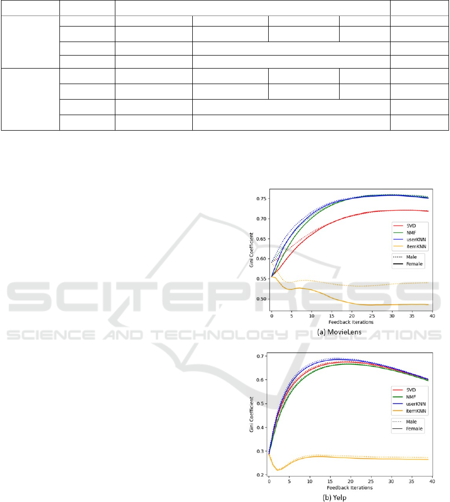
Table 2: RecSys model details.

Dataset Algorithm Optimal Hyperparameters RMSE

MovieLens SVD Epochs: 50 Factors: 150 LR: 0.005 RT: 0.05 0.90

NMF Epochs: 100 Factors: 150 0.89

userKNN K: 20 Metric: mean-squared deviation 0.95

itemKNN K: 75 Metric: mean-squared deviation 0.95

Yelp!

SVD Epochs: 10 Factors: 75 LR: 0.005 RT: 0.05 0.92

NMF Epochs: 100 Factors: 150 0.94

userKNN K: 50 Metric: mean-squared deviation 0.97

itemKNN K: 50 Metric: mean-squared deviation 0.97

Note: Epoch is a single pass through the dataset during training, factor the number of latent user and item factors used in

the model, learning rate (LR) the hyperparameter determining the size of the steps taken during optimisation affecting how

quickly the model converges, regularization term (RT) the penalty term added to the loss function to prevent overfitting, K

the number of neighbours that are taken into account for aggregation, and metric the method for distance computation.

4.3.1 Within-Group-Gini Coefficient

In this section, results of the metric within-group-Gini

coefficient is presented for two sensitive user groups,

males and females. Note, if a model consistently

provides fewer or more diverse recommendations to

a specific user group, it will lead to diverging values

of this metric between the groups. Figure 1 presents

the within-group-Gini coefficient of males and

females for the MovieLens and Yelp datasets. The

gap between the genders is visible more in

MovieLens than in Yelp due to larger preferential

differences between groups in movies than in their

choice of restaurants. Additionally, 4 observations are

made in Figure 1.

First, when evaluating differences between

genders, consistent trends across both datasets are

observed. Initially, in the first iteration, the metric’s

value for males is higher than for females. This

disparity is more prominent in the MovieLens dataset

(see Figure 1), but a similar trend also exists within

the Yelp dataset, although with a smaller difference.

These findings indicate that in the original dataset,

males have interacted with a smaller diversity of

items compared to females.

Second, in both datasets across both groups,

except for in itemKNN, the Gini coefficient increases

rapidly followed by an asymptote (MovieLens) or a

slow decline (Yelp). This is expected because over

time the propensity of recommending only popular

items increases. Hence the diversity of

recommendations decreases.

Figure 1: Results of within-group-Gini coefficient for male

and female over a feedback loop per RecSys model.

Third, the initial separation observed in values of

within-group-Gini coefficient between the groups

decreases over time, especially for MovieLens. This

implies that over time, males and females are

provided with increasingly similar recommendations

in terms of item diversity. This does not suggest that

ICAART 2024 - 16th International Conference on Agents and Artiﬁcial Intelligence

128

the recommended items are the same between the two

user groups, but the ascending order of distribution of

item popularity scores are similar.

Fourth, itemKNN’s behavorial difference

compared to the other algorithms is expected as

recommendations made in itemKNN are based on

similarity in item features and not on user similarity.

The difference between within-group-Gini coefficient

increases over time between the groups, suggesting

that over time, females are being recommended a

more diverse set of items compared to males.

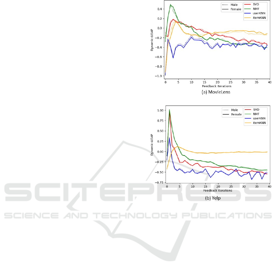
4.3.2 Dynamic-𝜟𝑮𝑨𝑷

When applying dynamic-𝛥𝐺𝐴𝑃, results (see Figure 2)

reveal extreme values in the initial iterations. This is

expected as user profiles are directly being compared

with recommendations provided in the first iteration.

It is also observed that initial values of dynamic-

𝛥𝐺𝐴𝑃 are negative, suggesting that the initial group-

recommendations were less popular than the average

user profiles of the respective group. This turbulent

starting phase is attributed to the "cold start" problem

within RecSys (Volkovs et al., 2017), where users

with relatively limited observed interactions in their

user profiles exert a significant influence on the

average popularity of their user group.

Except for itemKNN, the algorithms appear to

converge to a negative dynamic-𝛥𝐺𝐴𝑃 value. This

convergence to a negative value is because, SVD,

NMF and userKNN are prone to over recommending

popular items, which leads to an increase in the

average item popularity in the user profiles for the

initial iterations. After this initial phase these

algorithms are left with a pool of less popular items

to recommend. Hence, the average item popularity of

the recommended items after the initial phase is lower

than the average item popularity in the user profiles,

leading to the convergence of dynamic-𝛥𝐺𝐴𝑃 to a

negative value. On the contrary, itemKNN is based

on recommending items with similar features.

Therefore, over time it recommends similar items to

the user profiles. This leads to the average popularity

of the recommended items to be similar to the average

item popularity in the user profiles resulting in

dynamic-𝛥𝐺𝐴𝑃 converging towards zero.

Lastly, with regards to the sensitive user groups,

minor variations in dynamic-𝛥𝐺𝐴𝑃 is observed for

MovieLens dataset, however, for Yelp dataset this

variation is negligible. Similar to within-group-Gini

coefficient, this difference in the two datasets is due

to larger preferential differences between males and

females in movies than in their choice of restaurants.

Figure 2: Results of dynamic-ΔGAP for male and female

over a feedback loop per RecSys model.

4.3.3 Between-Group GAP

Between-group 𝐺𝐴𝑃 is demonstrated using six

hypothetical scenarios using ∆𝐺𝐴𝑃



in a

dynamic setting for male and female user groups.

Thereby, it is validated that over-recommendation of

popular items is more unfair than the over-

recommendation of non-popular items.

To illustrate this, six hypothetical scenarios are

presented in Table 3. In each scenario we first define

the difference of the item popularity within

recommendations compared to item popularity of

user profiles. To illustrate, an “ItemPopularity” of

+50% represents recommendations being 50% more

popular than their user profiles (e.g., 𝐺𝐴𝑃



=0.4

results in 𝐺𝐴𝑃



=0.6); an “ItemPopularity” of -50%

represents recommendations being 50% less popular

than their user profiles.

Metrics for Popularity Bias in Dynamic Recommender Systems

129

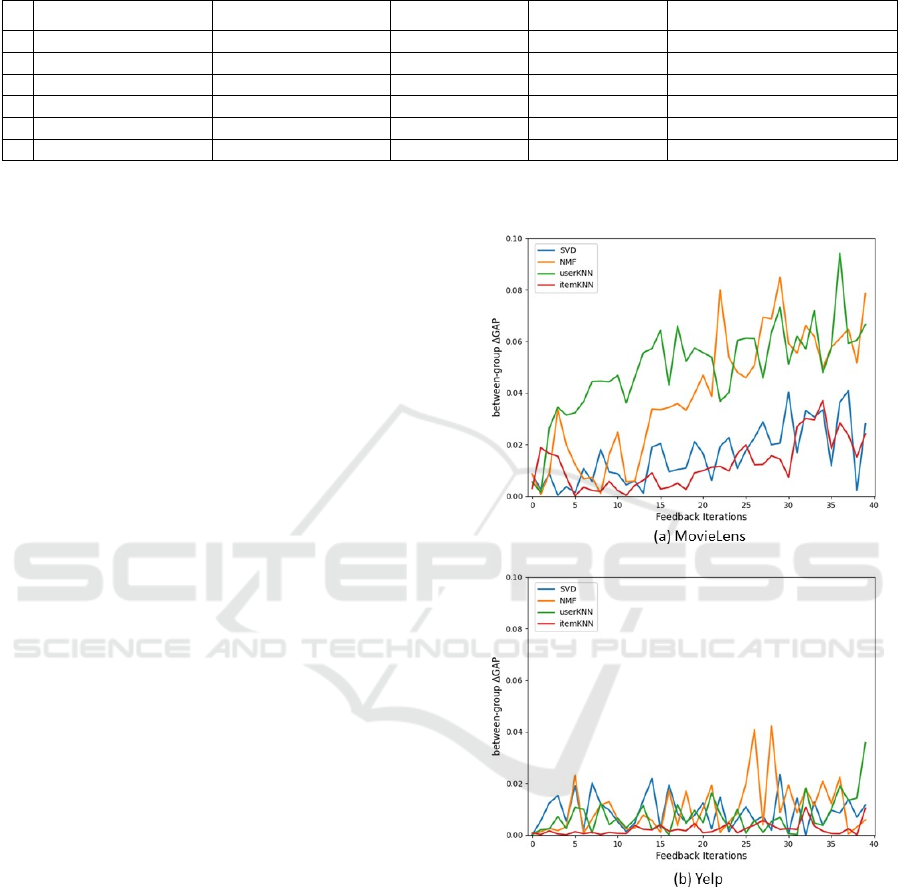
Table 3: Values of 𝐵𝑒𝑡𝑤𝑒𝑒𝑛−𝑔𝑟𝑜𝑢𝑝 𝐺𝐴𝑃 for different scenarios of over-recommending popular or non-popular items for

user groups 𝑔 and ℎ.

𝐈𝐭𝐞𝐦𝐏𝐨𝐩𝐮𝐥𝐚𝐫𝐢𝐭𝐲(𝐠) 𝐈𝐭𝐞𝐦𝐏𝐨𝐩𝐮𝐥𝐚𝐫𝐢𝐭𝐲(𝐡) ∆𝐆𝐀𝐏

𝐫𝐞𝐯𝐢𝐬𝐞𝐝

(𝐠) ∆𝐆𝐀𝐏

𝐫𝐞𝐯𝐢𝐬𝐞𝐝

(

𝐡

)

𝐁𝐞𝐭𝐰𝐞𝐞𝐧𝐆𝐫𝐨𝐮𝐩 𝐆𝐀𝐏(𝐠,𝐡)

1 + 50% + 50% 0.67 0.66 0.00

2 0% - 50% 1.00 1.33 0.28

3 0% + 50% 1.00 0.67 0.40

4 - 20% + 10% 1.13 0.93 0.19

5 - 10% + 20% 0.07 0.87 0.21

6 - 50% + 50% 1.33 0.67 0.67

Scenario 1 represents a perfect situation where

both groups g and h are treated equally with both

receiving recommendations that are 50% more

popular than their profiles. Scenarios 2 and 3

demonstrate how over-recommending popular items

is considered more unfair than over-recommending

unpopular items. In scenario 2, group g receives a

perfect recommendation and group h is recommended

items that are 50% less popular than their user

profiles, resulting in a 𝐵𝑒𝑡𝑤𝑒𝑒𝑛𝐺𝑟𝑜𝑢𝑝 𝐺𝐴𝑃 of

0.2857. In scenario 3, group g also receives a perfect

recommendation, but group h is recommended items

that are 50% more popular than their user profiles

instead, resulting in a 𝐵𝑒𝑡𝑤𝑒𝑒𝑛𝐺𝑟𝑜𝑢𝑝 𝐺𝐴𝑃 of 0.4.

Even though in both scenarios one group receives

recommendations that are 50% off their user profiles,

it illustrates that over-recommending popular items is

considered more unfair. Scenarios 4 and 5 illustrate

the same but with both groups receiving unfair

recommendations and for smaller differences

between groups.

The results of 𝐵𝑒𝑡𝑤𝑒𝑒𝑛𝐺𝑟𝑜𝑢𝑝 𝐺𝐴𝑃 for the

MovieLens and Yelp datasets are presented in Figures

3a and 3b, respectively. For the Yelp dataset,

consistent and relatively low values of the metric is

observed over time, indicating that all the four models

exhibit relatively low degree of unfairness towards

both males and females for the Yelp dataset.

However, the MovieLens dataset shows an increasing

trend in between-group unfairness, in particular for

userKNN and NMF models (see Figure 3a). These

models exhibit a distinct and noticeable pattern of

growing disparities in treatment between males and

females, resulting in a 𝐵𝑒𝑡𝑤𝑒𝑒𝑛𝐺𝑟𝑜𝑢𝑝 𝐺𝐴𝑃 value of

0.1. Referring to Table 3, a value of 0.1 indicates

group g receives perfect recommendations when

compared to their profiles (0% item popularity),

while group h receives recommendations that are

14.3% more popular than their profiles.

These findings highlight the metric's potential in

capturing and highlighting the emergence of unequal

treatment between sensitive user groups.

Furthermore, the metric demonstrates ability to

differentiate between the fairness-performance of the

four algorithms used in this study.

Figure 3: Results of between-group GAP for male and

female over a feedback loop per RecSys model.

4.3.4 Cosine Similarity

The proposed metric for popularity bias, cosine

similarity, measures the degree of similarity between

the frequency of recommended items among two user

groups. Values close to 1 represent a RecSys model

recommending items with similar frequencies

between user groups. Whereas values towards 0

represent the model recommending different items

between groups.

ICAART 2024 - 16th International Conference on Agents and Artiﬁcial Intelligence

130

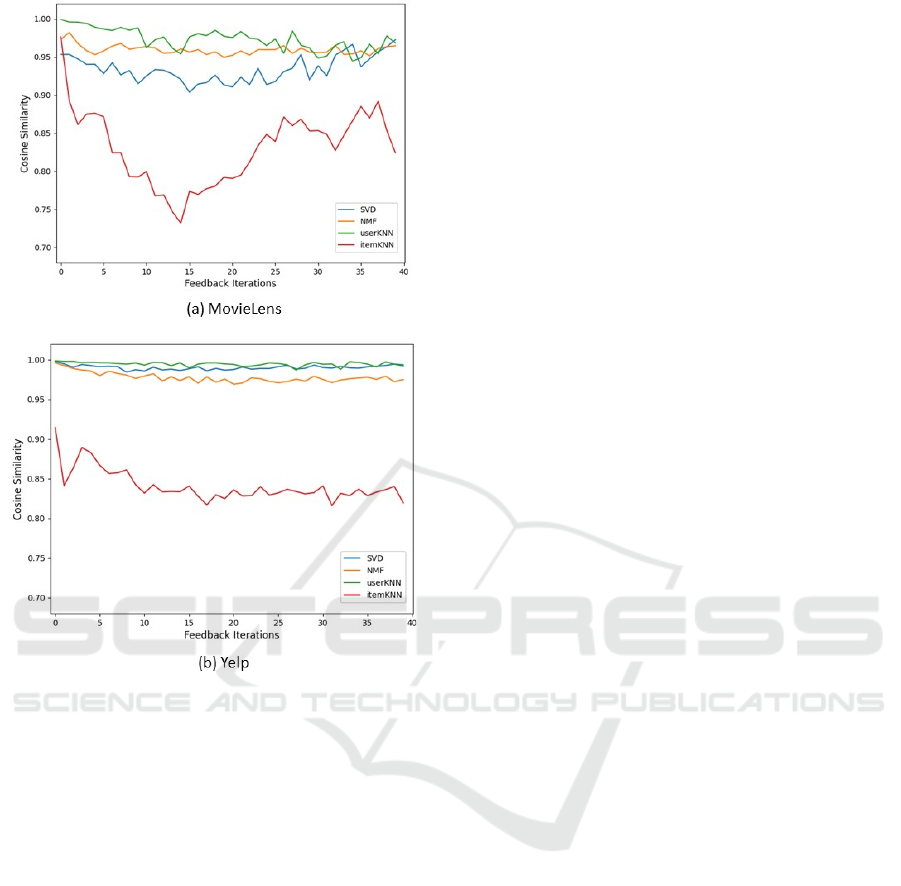
Figure 4: Results of cosine similarity for male and female

over a feedback loop per RecSys model.

Figure 4 presents the results for the MovieLens

and Yelp datasets. It is observed that the SVD, NMF,

and userKNN models have cosine similarity close to

1, indicating a high and stable degree of similarity in

recommendations between males and females over

time. Conversely, the results for itemKNN suggest

that the similarity of recommendations between

males and females decreases over time. The results of

itemKNN illustrate the importance of evaluating

RecSys in a dynamic setting, as the similarity in the

first iteration (i.e., a static setting) is significantly

higher than in later iterations. The results presented

demonstrate that the Yelp dataset presents more

stable results than the MovieLens dataset, providing

insights into the varying impact of different datasets

on the performance of RecSys models.

It is important to note that this Group-cosine

similarity has limitations due to potential differences

in preferences between groups, rendering it

insufficient as a standalone fairness metric.

Consequently, future research should consider

comparing the sorted normalised item popularity

distributions between groups. This will enable

evaluation of item popularity distributions among

groups and can potentially reveal if one user group is

presented with a more diverse set of items, offering

valuable insights into the extent of recommendation

diversity.

5 DISCUSSION & CONCLUSION

Popularity bias in RecSys leads to inequality in

treatment between users or user groups due to over-

recommendation of popular items. This bias arises

from the disproportionate favouring of popular items

leading to limited recommendation diversity and the

potential exclusion of relevant but less popular items

to certain users or groups. Therefore, it is important

to quantify and track such biases in RecSys.

The commonly used metrics to measure

popularity bias in RecSys are Gini coefficient, Delta

group average popularity (∆𝐺𝐴𝑃), and Generalized

entropy index ( 𝐺𝐸𝐼). Gini coefficient has been

deployed in more real-life dynamic setting which

quantifies inequality in the distribution of item

popularity scores over time (Chong & Abeliuk, 2019;

Zhu et al., 2021). However, this metric has only been

used at a global level thus undermining the

emergence of popularity bias between sensitive user

groups. 𝛥𝐺𝐴𝑃 , which measures the difference

between the average item popularity in user group-

recommendations and the average item popularity in

user group-profiles has only been used in literature in

static setting (Abdollahpouri et al., 2019). Biases in

RecSys generally creeps in over-time asymmetrically

in user groups, therefore it is important to extend the

application of 𝛥𝐺𝐴𝑃 not only to dynamic setting but

also to the context of different sensitive user groups.

𝐺𝐸𝐼 has been used to measure popularity bias both at

group levels and in dynamic setting, however, Gini

coefficient and 𝛥𝐺𝐴𝑃 are more commonly used due

to their interpretability.

To consider the time evolution of popularity bias

and its asymmetrical effects on different user groups,

four new metrics have been proposed, namely,

Within-group-Gini coefficient, Dynamic- 𝛥𝐺𝐴𝑃 ,

Between-group 𝐺𝐴𝑃, and Group-cosine similarity.

Within-group-Gini coefficient evaluates the equality

in the distribution of item popularities thus measuring

how diverse recommendations are over time between

sensitive user groups. Additionally, a new

methodology to compute 𝛥𝐺𝐴𝑃, Dynamic-𝛥𝐺𝐴𝑃,

has been proposed where recommendations provided

to the user are based on unobserved interactions in

contrast to the original proposal of Abdollahpouri et

Metrics for Popularity Bias in Dynamic Recommender Systems

131

al. (2019) and Kowald et al. (2020), in which users

are recommended items from the testing data which

they have already interacted with. The metric

𝐵𝑒𝑡𝑤𝑒𝑒𝑛𝐺𝑟𝑜𝑢𝑝 𝐺𝐴𝑃 measures popularity bias

resulting from the over-recommendation of popular

or non-popular items. The metric Group-cosine

similarity aims to assess the frequency of item

recommendations among different user groups,

specifically examining whether both groups are

recommended the same items in equal proportions

and can provide additional insights into the level of

between-group popularity bias in Recsys.

The proposed metrics have been demonstrated

using two commonly used datasets in academic

research on RecSys, namely the MovieLens 1M

dataset and the Yelp dataset with males and females

as sensitive user groups. It is worthwhile to note that

for a comprehensive understanding of time-evolution

of popularity bias for different sensitive user groups

in RecSys, it is advisable to use a combination of the

metrics proposed in this paper. For example, as

demonstrated in section 4, 𝐵𝑒𝑡𝑤𝑒𝑒𝑛𝐺𝑟𝑜𝑢𝑝 𝐺𝐴𝑃

metric highlighted a growing disparity in treatment

between males and females in the MovieLens dataset,

whereas, Within-group-Gini coefficient metric

revealed distinct trends in recommendation diversity

among different RecSys models. It is also observed

that the metric 𝐵𝑒𝑡𝑤𝑒𝑒𝑛𝐺𝑟𝑜𝑢𝑝 𝐺𝐴𝑃 demonstrates

ability to differentiate between the fairness-

performance of the four algorithms used in this study.

6 FUTURE WORK

Future work involves implementing and evaluating

the proposed metrics of popularity bias for more

advanced deep-learning based RecSys systems to

capture the complexity of industry-used models.

Furthermore, additional approaches of the proposed

metrics will be explored for their robust application,

such as comparing sorted normalised item popularity

distributions between different user groups to

compute cosine similarity and finding an optimal

method for incorporating 𝐺𝐴𝑃



in the calculation of

Dynamic-𝛥𝐺𝐴𝑃 as discussed in section 5.

REFERENCES

Abdi. H., (2010). Coefficient of variation. Encyclopedia of

research design 1 (pp. 169–171).

Abdollahpouri, H., & Mansoury, M. (2020). Multi-sided

Exposure Bias in Recommendation. In ACM KDD

Workshop on Industrial Recommendation Systems

2020.

Abdollahpouri, H., Mansoury, M., Burke, R., & Mobasher,

B. (2019). The Unfairness of Popularity Bias in

Recommendation. In 13th ACM Conference on

Recommender Systems, RecSys 2019.

Abdollahpouri, H., Mansoury, M., Burke, R., Mobasher, B.,

& Malthouse, E. (2021, June). User-centered evaluation

of popularity bias in recommender systems.

In Proceedings of the 29th ACM Conference on User

Modeling, Adaptation and Personalization (pp. 119-

129).

Adomavicius, G., & Tuzhilin, A. (2005). Toward the next

generation of recommender systems: A survey of the

state-of-the-art and possible extensions. IEEE

transactions on knowledge and data

engineering, 17(6), 734-749.

Ahanger, A. B., Aalam, S. W., Bhat, M. R., & Assad, A.

(2022, February). Popularity bias in recommender

systems-a review. In International Conference on

Emerging Technologies in Computer Engineering (pp.

431-444). Cham: Springer International Publishing.

Analytis, P.P., Barkoczi, D., Lorenz-Spreen, P., & Herzog,

S. (2020, April). The structure of social influence in

recommender networks. In Proceedings of The Web

Conference 2020 (pp. 2655-2661).

Aridor, G., Goncalves, D., & Sikdar, S. (2020, September).

Deconstructing the filter bubble: User decision-making

and recommender systems. In Proceedings of the 14th

ACM Conference on Recommender Systems (pp. 82-91).

Baeza-Yates, R. (2020, September). Bias in search and

recommender systems. In Proceedings of the 14th ACM

Conference on Recommender Systems (pp. 2-2).

Bhadani, S. (2021, September). Biases in recommendation

system. In Proceedings of the 15th ACM Conference on

Recommender Systems (pp. 855-859).

Chen, J., Dong, H., Wang, X., Feng, F., Wang, M., & He,

X. (2023). Bias and debias in recommender system: A

survey and future directions. ACM Transactions on

Information Systems, 41(3), 1-39.

Chen, J., Wang, X., Feng, F., & He, X. (2021, September).

Bias issues and solutions in recommender system:

Tutorial on the RecSys 2021. In Proceedings of the

15th ACM Conference on Recommender Systems (pp.

825-827).

Chong, S., & Abeliuk, A. (2019, December). Quantifying

the effects of recommendation systems. In 2019 IEEE

International Conference on Big Data (Big Data) (pp.

3008-3015). IEEE.

Collins, A., Tkaczyk, D., Aizawa, A., & Beel, J. (2018). A

study of position bias in digital library recommender

systems. arXiv preprint arXiv:1802.06565.

De Maio, F. G. (2007). Income inequality

measures. Journal of Epidemiology & Community

Health,

61(10), 849-852.

Deldjoo, Y., Jannach, D., Bellogin, A., Difonzo, A., &

Zanzonelli, D. (2023). Fairness in recommender

systems: research landscape and future directions. User

Modeling and User-Adapted Interaction, 1-50.

ICAART 2024 - 16th International Conference on Agents and Artiﬁcial Intelligence

132

Dwork, C., Hardt, M., Pitassi, T., Reingold, O., & Zemel,

R. (2012, January). Fairness through awareness.

In Proceedings of the 3rd innovations in theoretical

computer science conference (pp. 214-226).

Ekstrand, M. D., Tian, M., Azpiazu, I. M., Ekstrand, J. D.,

Anuyah, O., McNeill, D., & Pera, M. S. (2018,

January). All the cool kids, how do they fit in?:

Popularity and demographic biases in recommender

evaluation and effectiveness. In Conference on

fairness, accountability and transparency (pp. 172-

186). PMLR.

Gini, C. (1936). On the Measure of Concentration with

Special Reference to Income and Statistics. Colorado

College Publication, General Series No. 208, pp. 73-79.

Haughton, J., & Khandker, S. R. (2009). Handbook on

poverty+ inequality. World Bank Publications.

Khanal, S. S., Prasad, P. W. C., Alsadoon, A., & Maag, A.

(2020). A systematic review: machine learning based

recommendation systems for e-learning. Education and

Information Technologies, 25, 2635-2664.

Khenissi, S., Mariem, B., & Nasraoui, O. (2020,

September). Theoretical modeling of the iterative

properties of user discovery in a collaborative filtering

recommender system. In Proceedings of the 14th ACM

Conference on Recommender Systems (pp. 348-357).

Kirişci, M. (2023). New cosine similarity and distance

measures for Fermatean fuzzy sets and TOPSIS

approach. Knowledge and Information Systems, 65(2),

855-868.

Kordzadeh, N., & Ghasemaghaei, M. (2022). Algorithmic

bias: review, synthesis, and future research

directions. European Journal of Information

Systems, 31(3), 388-409.

Koren, Y., Bell, R., & Volinsky, C. (2009). Matrix

factorization techniques for recommender

systems. Computer, 42(8), 30-37.

Kowald, D., & Lacic, E. (2022, April). Popularity bias in

collaborative filtering-based multimedia recommender

systems. In International Workshop on Algorithmic

Bias in Search and Recommendation (pp. 1-11). Cham:

Springer International Publishing.

Kowald, D., Schedl, M., & Lex, E. (2020). The unfairness

of popularity bias in music recommendation: A

reproducibility study. In Advances in Information

Retrieval: 42nd European Conference on IR Research,

ECIR 2020, Lisbon, Portugal, April 14–17, 2020,

Proceedings, Part II 42 (pp. 35-42). Springer

International Publishing.

Lee, D., & Seung, H. S. (2000). Algorithms for non-

negative matrix factorization. Advances in neural

information processing systems, 13.

Leonhardt, J., Anand, A., & Khosla, M. (2018, April). User

fairness in recommender systems. In Companion

Proceedings of the The Web Conference 2018 (pp. 101-

102).

Lin, A., Wang, J., Zhu, Z., & Caverlee, J. (2022, October).

Quantifying and mitigating popularity bias in

conversational recommender systems. In

Proceedings

of the 31st ACM International Conference on

Information & Knowledge Management (pp. 1238-

1247).

Liu, Y., Cao, X., & Yu, Y. (2016, September). Are you

influenced by others when rating? Improve rating

prediction by conformity modeling. In Proceedings of

the 10th ACM conference on recommender systems (pp.

269-272).

Liu, D., Cheng, P., Dong, Z., He, X., Pan, W., & Ming, Z.

(2020, July). A general knowledge distillation

framework for counterfactual recommendation via

uniform data. In Proceedings of the 43rd International

ACM SIGIR Conference on Research and Development

in Information Retrieval (pp. 831-840).

Lü, L., Medo, M., Yeung, C. H., Zhang, Y. C., Zhang, Z.

K., & Zhou, T. (2012). Recommender systems. Physics

reports, 519(1), 1-49.

Lu, J., Wu, D., Mao, M., Wang, W., & Zhang, G. (2015).

Recommender system application developments: a

survey. Decision support systems, 74, 12-32.

Luong, B. T., Ruggieri, S., & Turini, F. (2011, August). k-

NN as an implementation of situation testing for

discrimination discovery and prevention.

In Proceedings of the 17th ACM SIGKDD international

conference on Knowledge discovery and data

mining (pp. 502-510).

Mansoury, M., Abdollahpouri, H., Pechenizkiy, M.,

Mobasher, B., & Burke, R. (2020, October). Feedback

loop and bias amplification in recommender systems.

In Proceedings of the 29th ACM international

conference on information & knowledge

management (pp. 2145-2148).

Marlin, B. M., Zemel, R. S., Roweis, S., & Slaney, M.

(2007, July). Collaborative filtering and the missing at

random assumption. In Proceedings of the Twenty-

Third Conference on Uncertainty in Artificial

Intelligence (pp. 267-275).

Mehrabi, N., Morstatter, F., Saxena, N., Lerman, K., &

Galstyan, A. (2021). A survey on bias and fairness in

machine learning. ACM computing surveys

(CSUR), 54(6), 1-35.

Mehrotra, R., McInerney, J., Bouchard, H., Lalmas, M., &

Diaz, F. (2018, October). Towards a fair marketplace:

Counterfactual evaluation of the trade-off between

relevance, fairness & satisfaction in recommendation

systems. In Proceedings of the 27th acm international

conference on information and knowledge

management (pp. 2243-2251).

Mussard, S., Seyte, F., & Terraza, M. (2003).

Decomposition of Gini and the generalized entropy

inequality measures. Economics Bulletin, 4(7), 1-6.

Oswald, M., Grace, J., Urwin, S., & Barnes, G. C. (2018).

Algorithmic risk assessment policing models: lessons

from the Durham HART model and

‘Experimental’proportionality. Information &

communications technology law, 27(2), 223-250.

Schäfer, H., Hors-Fraile, S., Karumur, R. P., Calero Valdez,

A., Said, A., Torkamaan, H., Ulmer, T. & Trattner, C.

(2017, July). Towards health (aware) recommender

systems. In Proceedings of the 2017 international

conference on digital health (pp. 157-161).

Metrics for Popularity Bias in Dynamic Recommender Systems

133

Shorrocks, A. F. (1984). Inequality decomposition by

population subgroups. Econometrica: Journal of the

Econometric Society, 1369-1385.

Singhal, A., Sinha, P., & Pant, R (2017). Use of Deep

Learning in Modern Recommendation System: A

Summary of Recent Works. International Journal of

Computer Applications, 975, 8887.

Speicher, T., Heidari, H., Grgic-Hlaca, N., Gummadi, K. P.,

Singla, A., Weller, A., & Zafar, M. B. (2018, July). A

unified approach to quantifying algorithmic unfairness:

Measuring individual &group unfairness via inequality

indices. In Proceedings of the 24th ACM SIGKDD

international conference on knowledge discovery &

data mining (pp. 2239-2248).

Steck, H. (2018, September). Calibrated recommendations.

In Proceedings of the 12th ACM conference on

recommender systems (pp. 154-162).

Sun, W., Khenissi, S., Nasraoui, O., & Shafto, P. (2019,

May). Debiasing the human-recommender system

feedback loop in collaborative filtering. In Companion

Proceedings of The 2019 World Wide Web

Conference (pp. 645-651).

Theil, H. (1967). Economics and Information Theory.

North Holland, Amsterdam.

Vogiatzis, D., & Kyriakidou, O. (2021). Responsible data

management for human resources. In Proceedings of

the First Workshop on Recommender Systems for

Human Resources (RecSys in HR 2021) co-located with

the 15th ACM Conference on Recommender Systems

(RecSys 2021) (Vol. 2967).

Volkovs, M., Yu, G., & Poutanen, T. (2017). Dropoutnet:

Addressing cold start in recommender

systems. Advances in neural information processing

systems, 30.

Wang, Y., Ma, W., Zhang, M., Liu, Y., & Ma, S. (2023). A

survey on the fairness of recommender systems. ACM

Transactions on Information Systems, 41(3), 1-43.

Wundervald, B. (2021). Cluster-based quotas for fairness

improvements in music recommendation

systems. International Journal of Multimedia

Information Retrieval, 10(1), 25-32.

Yalcin, E., & Bilge, A. (2021). Investigating and

counteracting popularity bias in group

recommendations. Information Processing &

Management, 58(5), 102608.

Zehlike, M., Yang, K., & Stoyanovich, J. (2022). Fairness

in ranking, part ii: Learning-to-rank and recommender

systems. ACM Computing Surveys, 55(6), 1-41.

Zemel, R., Wu, Y., Swersky, K., Pitassi, T., & Dwork, C.

(2013, May). Learning fair representations.

In International conference on machine learning (pp.

325-333). PMLR.

Zhao, Z., Chen, J., Zhou, S., He, X., Cao, X., Zhang, F., &

Wu, W. (2022). Popularity bias is not always evil:

Disentangling benign and harmful bias for

recommendation.

IEEE Transactions on Knowledge

and Data Engineering.

Zhu, Z., He, Y., Zhao, X., & Caverlee, J. (2021, August).

Popularity bias in dynamic recommendation.

In Proceedings of the 27th ACM SIGKDD Conference

on Knowledge Discovery & Data Mining (pp. 2439-

2449).

ICAART 2024 - 16th International Conference on Agents and Artiﬁcial Intelligence

134