Real-Time Desertscapes Simulation with CUDA

Alexander Maximilian Nilles

, Lars G

unther and Stefan M

uller

Institute for Computational Visualistics, University of Koblenz, Universit

atsstr. 1, Koblenz, Germany

Keywords:

Procedural Modeling, Desert, Sand-Dunes, Simulation, Aeolian Erosion, Real-Time, GPU, CUDA.

Abstract:

We propose a new GPU-based method capable of simulating dune formation, propagation and aeolian sand

transport, based on the Desertscape Simulation model. Our method improves upon the original as well as an

existing real-time GPU implementation by introducing bilinear interpolation and removing randomness, which

leads to a more robust and noise-free method. We implement our method with CUDA and use atomic adds on

ﬂoats to remove a previous limitation that required block-based discretization of elevation values. A new sand

distribution scheme for sand avalanching is proposed that converges faster than the previous work. We propose

and evaluate a new method for reptation, which was previously neglected. Our method further improves on the

performance compared with the previous real-time method and can generate results that more closely resemble

dune evolution with a bidirectional wind scheme as predicted by an accurate ofﬂine method. Our method can

generate detailed, physically plausible desert environments very quickly, with possible applications in both

computer graphics as well as geomorphology. With some restrictions, our method could even be used during

gameplay.

1 INTRODUCTION

Terrain modeling in computer graphics has seen a lot

of focus on hydraulic erosion, as water-based pro-

cesses are very common for typical landscapes and

mountain ranges. In deserts, erosion is however pre-

dominantly driven by wind. Due to effects such as

wind shadowing, many different types of sand dunes

can form. Depending on sand availability, wind con-

ditions and the presence of vegetation, we can en-

counter crescent-shaped barchan dunes, transverse

dunes, star-shaped dunes or anchored nabhka dunes.

The underlying terrain further inﬂuences wind, is

abraded by the sand and steep cliffs can lead to the

formation of echo dunes.

Aside from generating small-scale sand ripples,

proper simulation of dunes was restricted to expen-

sive ofﬂine models used in geomorphology for a long

time. With the introduction of the Desertscapes Sim-

ulation model (Paris et al., 2019), physically plausi-

ble dune simulation and aeolian sand transport be-

came feasible for computer graphics. The CPU-based

method, while not real-time, was fast enough to rea-

sonably be used for interactive terrain modeling.

In this paper, we present a novel real-time ex-

tension of the Desertscapes Simulation implemented

https://orcid.org/0000-0002-4196-7424

in CUDA. Our method introduces various improve-

ments over the original, as well as an existing real-

time GPU implementation that was independently de-

veloped earlier (Taylor and Keyser, 2023), further im-

proving both performance and detail of the results.

Our main contributions are 1) removal of a restric-

tion requiring elevation values to be stored as inte-

gers, greatly simplifying the algorithm; 2) usage of

bilinear interpolation instead of nearest neighbor se-

lection in wind shadow calculation, advection and the

generation of cliff cells for echo dunes, resulting in a

more robust method and smoother results; 3) removal

of the random nature of the original algorithm, re-

sulting in a noise-free, deterministic method; 4) an

improved sand distribution scheme for avalanching

that converges faster; 5) a new method for handling

reptation, which provides a big impact on simulation

results, unlike previous work. We compare our re-

sults with an ofﬂine simulation as done in (Taylor and

Keyser, 2023).

Section 2 will introduce relevant related work

concerning erosion and sand simulation in computer

graphics and geomorphology. In Section 3 we outline

our method and the various changes to previous work

and Section 4 will further explain key implementation

details. We evaluate our method and the changes we

made to the algorithm in Section 5, comparing to the

previous GPU implementation. Section 6 concludes

Nilles, A., Günther, L. and Müller, S.

Real-Time Desertscapes Simulation with CUDA.

DOI: 10.5220/0012315600003660

Paper published under CC license (CC BY-NC-ND 4.0)

In Proceedings of the 19th International Joint Conference on Computer Vision, Imaging and Computer Graphics Theory and Applications (VISIGRAPP 2024) - Volume 1: GRAPP, HUCAPP

and IVAPP, pages 34-45

ISBN: 978-989-758-679-8; ISSN: 2184-4321

with a summary, important limitations as well as top-

ics for further research.

We provide our entire source code in the sup-

plementary materials of this paper and additionally

make it available open source on GitHub (Nilles and

unther, 2023).

2 RELATED WORK

Generating realistic landscapes by hand is time-

intensive and tedious, thus terrain modeling is a vast

and important ﬁeld of research in computer graphics.

Early techniques include procedural generation using

noise (Mandelbrot and Van Ness, 1968; Musgrave

et al., 1989), while other approaches involve simula-

tion or example-based terrain generation (Galin et al.,

2019). We will mainly focus on interactive and real-

time simulation techniques and methods that specif-

ically target deserts, aeolian erosion and sand dunes.

For an overview of the geomorphology of dunes and

desert landscapes, we refer to the literature (Lan-

caster, 2013; Livingstone and Warren, 2019).

2.1 Hydraulic Erosion

Aeolian erosion shares similarities with hydraulic

erosion, as both wind and water are ﬂuids that remove

material and then transport it, depositing it elsewhere.

This makes such simulation methods particularly in-

teresting, since some ideas can potentially be reused.

Hydraulic erosion has been researched extensively in

computer graphics, more so than aeolian erosion.

(Mei et al., 2007) introduced a real-time hydraulic

erosion simulation based on heightmaps. Their

method is designed for the GPU and can simulate ero-

sion of mountain landscapes by rain and rivers, yield-

ing plausible and visually interesting results.

(

St’ava et al., 2008) propose another GPU-based

real-time simulation which supports multiple layers

of different materials and models both dissolution and

force-based erosion effects. They also support terrain

avalanching with a varying angle of repose based on

the presence of water.

Other methods such as (Kri

stof et al., 2009) model

water fully 3D using particles with the Smoothed Par-

ticle Hydrodynamics method instead of using a 2D

heightmap as in the previous approaches, providing

more realism in terms of ﬂuid behavior.

2.2 Aeolian Erosion

(Rozier and Narteau, 2014) developed the Real-Space

Cellular Automaton Laboratory (ReSCAL). They use

a cellular autonoma model which describes the scene

in 3D using voxels. The model is driven by a given

voxel’s state which undergoes state transitions based

on the state of neighboring voxels and a stochasti-

cally driven event-based model. ReSCAL is a gen-

eral model for computational geomorphology and can

be used for dune morphodynamics, similar to previ-

ous work (Zhang et al., 2010). The method has been

proven to accurately model sand dune formations and

has been used to drive further research in geomor-

phology such as (Gao et al., 2015; L

u et al., 2018). A

more recent model called ReSCAL-Snow (Kochan-

ski et al., 2019a) can also simulate snow dunes and

was used to generate training data for deep learning.

While ReSCAL is very accurate, it is too slow to be

used in a computer graphics context, whether to au-

thor a static terrain or an animated one (Kochanski

et al., 2019b).

Early work on aeolian erosion for computer

graphics mainly focused on small scale sand rip-

ples (Bene

s and Roa, 2004; Wang and Hu, 2009),

including handling of obstacles and later vegetation.

While these methods can run in real-time and gener-

ate convincing results, albeit not physically accurate

ones, they are not suited for large dune formations.

Later work (Wang and Hu, 2012) proposed an exten-

sion for larger terrains by applying the algorithm in

a hierarchical manner at larger scales, i.e. generating

dunes based on their similarity to small sand ripples.

The ﬁrst method suitable for computer graphics

that was capable of generating large-scale desert land-

scapes was (Paris et al., 2019). Their method can gen-

erate many different types of dunes such as barchan-,

star-, nabhka and transverse dunes. It handles salta-

tion, reptation and avalanching along with aeolian

bedrock erosion all in one framework. The salta-

tion process is modeled event-driven, where events

such as sand lifting, deposition, bounces and reptation

are sampled stochastically. Their method was imple-

mented on the CPU, but is well-suited for paralleliza-

tion on the GPU. Alongside with the convincing re-

sults, we thus decided to base our own real-time GPU

simulation on their method.

Independently from us, (Taylor and Keyser, 2023)

worked on their own real-time GPU implementation

of the Desertscapes model. They proposed a straight-

forward parallelization of the original work, keeping

the stochastic nature of the saltation process. Due to a

lack of atomic operations on ﬂoating-point numbers

in Direct3D, terrain elevation was discretized into

discrete blocks stored as integers. Unlike the orig-

inal work, avalanching is not executed in an event-

based manner. Instead of detecting all necessary

avalanching events and recursively resolving all of

Real-Time Desertscapes Simulation with CUDA

them, which is unsuitable for parallel GPU implemen-

tations, they implement the algorithm iteratively and

make sure to execute enough iterations to reach con-

vergence. Furthermore, they extend the original ap-

proach, adding a solution for echo dunes formation

around obstacles which is based on wind tunnel ex-

periments (Tsoar, 1983). They evaluate their work

against wind tunnel simulations as well as ReSCAL

simulation results and show that the method produces

realistic results, albeit struggling to reproduce the ex-

pected results in situations of low sand availability.

3 OUR METHOD

In this section, we will explain our method, highlight-

ing the parts that differ from the original Desertscape

Simulation (Paris et al., 2019) and the previously

developed GPU implementation (Taylor and Keyser,

2023). We outline the full method for clarity, but will

only explain the unchanged portions brieﬂy, referring

the reader to the previous work.

3.1 Discretization

While (Paris et al., 2019; Taylor and Keyser, 2023)

only support square resolutions, our simulation works

on a N ×M 2D grid of cells with periodic boundaries,

where each cell has a width of l meters. For every

cell i

i = (x, y), we store bedrock height b(i

i) ∈ (−∞,∞)

and sand height s(i

i) ∈ [0,∞) as heightmaps in meters,

where sand is always on top of bedrock. The com-

bined height is h(i

i) = b(i

i) + s(i

i). Unlike (Taylor and

Keyser, 2023), we store all quantities as ﬂoating-point

numbers and require no discretization of height into

blocks of ﬁxed size. This is possible because CUDA,

unlike the compute shaders used in the previous work,

is capable of atomic adds on ﬂoating-point numbers.

Following (Paris et al., 2019), we furthermore

store vegetation density r

i) ∈ [0,1] and bedrock ero-

sion resistance r

i) ∈ [0, 1] for each cell. These quan-

tities remain unchanged throughout the simulation.

3.2 Algorithm Overview

Each simulation step uses the previously described

quantities alongside a time-varying high altitude wind

velocity w

and time step ∆t as input and computes

the new bedrock and sand height values for the next

time step. The main steps of the algorithm are as fol-

lows:

1. Wind Warping

2. Wind Shadow

3. Echo Dunes

4. Saltation

5. Reptation

6. Avalanching

Figure 1 shows a simpliﬁed overview of the core sand

transport loop used in our method.

3.3 Wind Warping

Since a uniform wind direction for each cell on a

large terrain is unrealistic, (Paris et al., 2019) pro-

posed a simple wind warping scheme that accounts

for venturi effects (Equation (1)) and warps the wind

direction based on the gradient of the terrain (Equa-

tion (2)). (Taylor and Keyser, 2023) note that this

scheme is fairly simplistic, but opted to use it as well

with only minor modiﬁcations as it works well in a

real time setting. While we experimented with adding

a projection step to the proposed scheme, yielding a

divergence-free (mass-conserving) wind ﬁeld (Stam,

1999), we discarded the idea for increased perfor-

mance, since the effects of wind warping are com-

paratively minor in most scenes.

Venturi effects are accounted for by scaling wind

velocity based on terrain height

v(i

i) = w

(1 + k

h(i

i)) (1)

with k

= 5 · 10

−3

. With h

i) deﬁned as the terrain

height convolved with a Gaussian of radius r meters

(we use r = 2σ), the warped wind ﬁeld is computed

according to Equations (2) and (3):

i) = 0.2 f

i) ◦ v

v(i

i) + 0.8 f

200

◦ v

v(i

i) (2)

i) ◦ v

v(i

i) = (1 − α)v

v(i

i) + αk

∇h

⊥

i) (3)

with k

= 5 and k

200

= 30. While our implemen-

tation is general enough to support any set of param-

eters and up to four different Gaussians, we use the

same parameters proposed in (Paris et al., 2019) and

refer to their paper for further information.

Note that in Equation (3), α is computed as the

length of ∥∇h

∥, thus α can be larger than 1. We

modify the original approach and clamp α to 1. In

situations with very steep cliffs, such as the scenes

proposed in (Taylor and Keyser, 2023) for their wind

tunnel experiments, gradients can become fairly large

and cause wind to completely avoid the obstacle,

causing their proposed method for echo dunes (see

Section 3.5) to have no effect. We alleviate this by

scaling gradients by a user-deﬁned constant k

which

is set to 1 unless otherwise mentioned. Addition-

ally, Equation (2) does not preserve the length of v

v(i

and can result in larger or smaller wind velocities. For

this reason we compute the ﬁnal w

w(i

i) by restoring

i) to be of length ∥v

v(i

i)∥.

GRAPP 2024 - 19th International Conference on Computer Graphics Theory and Applications

Figure 1: An overview of the sand transport used in our

method, simpliﬁed to 1D. The ﬁgure shows the cell grid in-

cluding bedrock, sand and vegetation. The slab buffer s

shown above the grid and the reptation buffer s

is shown

below. A more saturated shade of yellow is used to indicate

transported sand. 1) Sand is lifted from all cells in paral-

lel and stored in the slab buffer. For clarity, only two cells

are considered here. The amount of lifted sand depends

on wind shadow, vegetation density and the sticky/erosion

property of a cell. After lifting, the slab buffer is advected

forward according to the wind using bilinear interpolation.

2) The slab buffer is copied to the reptation buffer. Then,

sand is deposited from the slab buffer to the terrain. The

deposited portion depends on wind shadow, vegetation and

sticky/erosion/object properties. Sand that is not deposited

bounces, which means it stays in the slab buffer. 3) The

reptation buffer is read to control the strength of reptation,

which moves sand downwards to neighboring cells. Down-

ward slopes that exceed the angle of repose are then stabi-

lized using avalanching.

3.4 Wind Shadow

(Paris et al., 2019; Taylor and Keyser, 2023) compute

wind shadowing by stepping upwind up to a maxi-

mum distance, keeping track of the maximum eleva-

tion difference. They then compute the angle based

on the found difference, where angles of less than 10

◦

resolve to no wind shadowing and angles above 15

◦

are fully shadowed.

Note that the maximum elevation difference does

not necessarily ﬁnd the maximum angle for the wind

shadow. We observed that using the maximum angle

led to better results. In linear mode, we ﬁnd the max-

imum angle as

tanα(i

i) = max

j=1,...,N







i − j

w(i

∥w

w(i

i)∥



− h(i

j · l





(4)

by stepping a maximum of N

= 10m/l cells, with

each step as long as the width of cells. To the best of

our knowledge, (Paris et al., 2019; Taylor and Keyser,

2023) snap to nearest neighbors in their method. We

instead sample the heightﬁeld with bilinear interpo-

lation in Equation (4). In curved mode, instead of

stepping upwind with the wind direction at the initial

cell, we update the wind direction at every step, tak-

ing a bilinear sample of the wind ﬁeld at that position,

which is more accurate for scenes with highly varying

wind directions.

Using Equation (4), we then compute the wind

shadow r

i) ∈ [0, 1] as the linear interpolation be-

tween tan 10

◦

and tan 15

◦

, similar to (Paris et al.,

2019).

3.5 Echo Dunes

In order to better compare our performances, we

implement the proposed method from (Taylor and

Keyser, 2023) for handling echo dunes with small

modiﬁcations, using the same default parameters but

adapted to our ﬂoating-point representation. For a de-

tailed explanation of the method and motivation, we

refer to the original work. We store the classiﬁca-

tion into erosion and sticky cells as r

i), where ero-

sion cells are encoded as negative values, while sticky

cells are encoded as their positive percentage as in the

original work. Furthermore, we implement the same

linear and curved modes from Section 3.4 and use bi-

linear interpolation instead of nearest neighbor in the

computation of cliff cells. For the classiﬁcation into

erosion and sticky cells, we found no beneﬁts with bi-

linear interpolation, so we use nearest neighbor as in

the original work, which is also much cheaper to com-

pute due to the high number of samples taken in this

step. We encode the object map by storing negative

values for the vegetation density where there are ob-

jects to save memory. As sand is never deposited on

top of objects and no avalanching is applied to them,

there is no point to vegetation density on top of them,

so we lose no functionality.

Real-Time Desertscapes Simulation with CUDA

3.6 Saltation

The saltation step of the algorithm handles the lifting

of sand by the wind, the advection of said sand along

the wind direction and subsequent deposition and

bouncing events. Both (Paris et al., 2019) and (Taylor

and Keyser, 2023) model this process using random

events. They assign a probability to each event, gener-

ate a random number and then only execute the event

with the given probability, moving a ﬁxed quantity of

sand in the process.

We use a different approach to saltation that does

not use a stochastic process, which is possible in our

GPU implementation as we are using ﬂoats instead of

integers. Instead of moving a quantity of sand x with

probability p, we simply move p · x, i.e. the expected

value, while the remaining (1 − p) · x are attributed to

the situation where the event does not occur. Instead

of only executing one of the possible events, we thus

handle all of them at once with the appropriate prob-

abilities.

First, we calculate the amount of sand to be lifted

based on slab size ε

, wind shadow and vegetation

density as

· (1 − r

i)) · (1 − r

i)). (5)

We use ε

= 1 if not speciﬁed otherwise. Equation (5)

is further multiplied by 0.5 if the cell is sticky and we

add k

= 1 if the cell is an erosion cell to support echo

dunes as described in (Taylor and Keyser, 2023). We

also limit the amount of lifted sand to the available

quantity of sand in the cell.

The lifted sand is then subtracted from the cell

and added on top of the slab buffer s

i), which is

initially empty. We then advect the slab buffer us-

ing forward advection, shifting values by w

w(i

i) · ∆t/l

cells, using bilinear interpolation in the process. This

is in contrast to (Paris et al., 2019; Taylor and Keyser,

2023), who use nearest neighbor, causing advection

to fail for very small wind speeds. Additionally, they

perform this advection step multiple times, up to a

maximum number of bounces, checking for deposi-

tion events each time. We only perform one step in

each loop of the algorithm. Sand that bounces in-

stead of being deposited is left in the slab buffer,

thus supporting theoretically inﬁnite bounces. Our

approach resembles typical advection in physics sim-

ulations. While we would have preferred to use the

backward Euler method, this was not an option since

the wind velocity ﬁeld after wind warping is not mass-

conserving, which would lead to errors (Stam, 1999).

After advection, we calculate the deposition prob-

ability based on wind shadow, vegetation, stickiness

of the cell and whether it is an object or erosion cell,

as described in previous work (Paris et al., 2019; Tay-

lor and Keyser, 2023). We use the deposition prob-

ability as a percentage as described above, removing

the corresponding portion of sand from the slab buffer

and adding it onto the cell. The sand remaining in the

slab buffer is thus the sand that bounced instead of

being deposited.

In (Paris et al., 2019), bounces during saltation

trigger abrasion of bedrock if the sand layer is below

a threshold, transforming a small amount of bedrock ε

into sand. We calculate this amount as described

in the original work, scaling it with the remaining

amount of sand in the slab buffer after deposition,

which indicates how much sand bounced on this cell.

Both deposition as well as bounces trigger repta-

tion events in the original work, where the probabil-

ity of a reptation event further depends on the veg-

etation density. We store the sum of deposited and

bounced sand as s

i) scaled by 1 − r

i) to incorpo-

rate this into our method, where s

is used to indi-

cate the strength of reptation in the next step of our

method.

3.7 Reptation

While the original Desertscapes Simulation handles

reptation in their method, neither (Paris et al., 2019)

nor (Taylor and Keyser, 2023) discussed reptation in

their results. Analysis of the sample code provided

in (Paris, 2022, desert-simulation.cpp, lines 157-160)

showed a comment mentioning that the author did not

observe any difference with reptation enabled or dis-

abled. Based on the included code, the reason for this

was that the implementation only moves sand down

slopes that exceed the angle of repose, functioning

nearly identical to avalanching, thus resulting in no

visible difference.

We remove this existing ﬂaw, allowing reptation

to move sand downward along any slope, no matter

the angle. We calculate the sand transfer between two

cells i

i and j

j by ﬁrst computing the height difference,

normalized to grid coordinates

d(i

i, j

j) =

h( j

j) − h(i

l · ∥i

i − j

j∥

. (6)

Equation (6) has the useful symmetry property

where d(i

i, j

j) = −d( j

j, i

i), which allows us to indepen-

dently calculate reptation for each cell, obtaining the

same magnitudes on receiving cells as on donating

cells without the need for any atomics. We scale this

quantity using the mean of both cell’s reptation values

that were computed in the saltation step.

i, j

j) = k

· |d(i

i, j

j)| ·

i) + s

( j

j)) . (7)

GRAPP 2024 - 19th International Conference on Computer Graphics Theory and Applications

in Equation (7) controls the overall strength of the

reptation effect. In order to account for sand avail-

ability, we restrict s

to the amount of available sand,

based on whether the cell is receiving or donating in

order to maintain the aforementioned symmetry prop-

erty.

⋆

i, j

j) =

(

min(s

i, j

j), s( j

j)) if d(i

i, j

j) ≥ 0

−min(s

i, j

j), s(i

i)) if d(i

i, j

j) < 0

(8)

For each cell, we calculate the mean of Equation (8)

across its 8 neighbors and add it to the current sand

height in the cell.

3.8 Avalanching

We follow the approach in (Taylor and Keyser, 2023)

where avalanching is implemented by iteratively dis-

tributing sand downward to the 8 neighboring cells

for all cells in parallel, typically using 50 total itera-

tions. This is in contrast to the original work, which

only updates a single cell at a time and then fully sta-

bilizes that cell and all neighboring cells, adding cells

that need further stabilization into a queue until the

queue is empty. Thus, our method has no guarantee

of fully converging and requires careful selection of

the number of necessary iterations based on the scene

parameters, as explained in more detail in (Taylor and

Keyser, 2023).

In each iteration, (Taylor and Keyser, 2023) dis-

tribute sand in proportion to the tangent of angles to

neighboring cells which exceed the angle of repose.

The total amount of sand moved is set to be equiva-

lent to the maximum found height difference, scaled

by k

= 0.25 to avoid oscillations. For details of their

approach, we refer to the original work. We adapt

their approach to our method which uses ﬂoats, re-

moving the need for discretization into blocks and

compare our own method to this algorithm.

We propose a different scheme for sand distribu-

tion in each avalanching loop, which converges faster.

Instead of distributing based on the tangent angle, we

ﬁrst calculate the exact amount of sand that is above

the angle of repose

B(i

i, j

j) = max((d( j

j, i

i) − tan θ

) · l · ∥i

i − j

j∥, 0), (9)

where tanθ

is linearly interpolated based on vege-

tation density between tan 33

◦

and tan 45

◦

(Beakawi

Al-Hashemi and Baghabra Al-Amoudi, 2018; Paris

et al., 2019). Equation (9) is then summed over

all 8 neighboring cells, yielding B

sum

i) while keep-

ing track of the maximum value for all neigh-

bors, B

max

i). The percentage of the total amount of

sand moved to neighbor j

j is then deﬁned as p(i

i, j

j) =

B(i

i, j

j)/B

sum

i).

We calculate the total amount of sand B

i) to

move away from i

i as the exact amount needed to sta-

bilize the neighbor that requires the most amount of

sand to reach the angle of repose (B

max

), restricted to

the amount of available sand. Note that our B

max

different from the one in (Taylor and Keyser, 2023),

where it is instead the maximum elevation difference.

To achieve this, ﬁrst consider that the elevation of i

will decrease by B

, while the target neighboring cell

will increase by B

max

sum

, i.e. we want to satisfy

max

= B



1 +

max

sum



(10)

solving Equation (10) and restricting by available

sand yields Equation (11)

i) = min





max

1 +

max

sum

,s(i





. (11)

The sand distributed from i

i to j

j is then k

· p(i

i, j

j) ·

i), where we use the k

parameter which is analo-

gous to (Taylor and Keyser, 2023). We ﬁnd that k

= 1

is stable but leads to very small artifacts which disap-

pear as the algorithm converges and will not be no-

ticeable if sufﬁcient iterations are used. Nevertheless,

we address these artifacts by using k

= 0.5 for a sub-

set of iterations, which is in contrast to the previous

method which uses k

= 0.25 for all iterations.

Avalanching is mainly used to stabilize the sand

layer. We optionally apply a single iteration of the

avalanching algorithm to the bedrock layer, where an-

gles are calculated using only the bedrock height, not

the total elevation, with an angle of repose of 68

◦

This is only needed if a lot of abrasion happens, ei-

ther due to setting a high abrasion strength or when

simulating for a very long time, smoothing results.

Bedrock moved during this process can optionally be

transformed into sand.

4 IMPLEMENTATION

We implement our method on the GPU using CUDA,

combined with OpenGL in order to visualize re-

sults in real time. The sand and bedrock elevation

map is allocated as a 2-component ﬂoating point tex-

ture in OpenGL, along with the resistance map, a

4-component ﬂoating-point texture that stores wind

shadow, vegetation density, bedrock erosion resis-

tance and stickiness. All other necessary buffers and

textures are directly allocated in CUDA.

Real-Time Desertscapes Simulation with CUDA

4.1 Visualization

For our visualization, we render a coarse ﬂat grid

which is further tesselated to N × M in the tesselation

stage. The tesselation evaluation shader then reads

sand and bedrock elevation values and computes the

height of each vertex along with its normal for shad-

ing accordingly. In the fragment shader, we imple-

ment a simple phong model with no shadows. The

diffuse material color of a cell is then set to grey if

no sand is present and darkened with increased ero-

sion resistance. We interpolate toward the sand color

across a small interval of sand elevation values. If

there is vegetation present, the color is further inter-

polated towards green. If the cell is part of the object

map, we set the color to purple. This color is then illu-

minated and further mixed with red for wind shadow,

blue for erosion cells and yellow for sticky cells.

Additionally, an overlay UI can be used to control

the simulation as well as the colors used in visualiza-

tion. Most parameters of the simulation can be set

here and changed during runtime of the simulation,

with some exceptions like the resolution requiring to

restart the simulation with a button. The UI allows

to export and to load all parameters to/from JSON,

along with the elevation and resistance maps saved

as EXR ﬁles. Most of the scenes used for this paper

are included in the supplementary material and our

GitHub repository (Nilles and G

unther, 2023) to facil-

itate better reproducibility. Elevation maps and resis-

tance maps can also be initialized with a very simple

procedural noise directly in the UI. The UI addition-

ally keeps track of performance metrics which we use

in our evaluation.

4.2 Simulation

The entire method as described in Section 3 is ex-

ecuted every frame in CUDA. Elevation and resis-

tance maps are mapped to CUDA beforehand, and

unmapped once all kernels are ﬁnished. Both of these

operations force a synchronization between OpenGL

and CUDA. Wind shadow calculation is fairly trivial

to parallelize, but all the other steps in our method

contain some noteworthy implementation details. For

more information, we refer to the source code in the

supplementary material or on GitHub.

4.2.1 Wind Warping

Wind Warping is straightforward to parallelize since

there are no race conditions, as the wind values at a

cell are independent from neighboring wind values

and the terrain does not change. However, wind warp-

ing uses large gaussian ﬁlters which can be a big per-

formance bottleneck. Fortunately, our grid uses peri-

odic boundaries so we can apply the convolution the-

orem.

We precompute the necessary Gaussians without

cutting them off at their radius, i.e. we write values for

the whole resolution. The result is normalized to have

a sum of 1 using a reduction operation. We then apply

an fftshift to this, which means that we do not need to

fftshift the terrain during runtime. The discrete fast

fourier transform of this is then calculated in-place

using the cuFFT library.

At runtime, we ﬁrst ﬁll a buffer with the total el-

evation. The FFT is then calculated in-place and we

perform a component-wise complex multiplication of

this spectrum with the precomputed spectrum of the

Gaussian, applying the inverse FFT afterwards, which

results in the smoothed terrain that we need for wind

warping.

4.2.2 Echo Dunes

The original approach from (Taylor and Keyser, 2023)

steps upwind starting from cliff cells, marking cells as

erosion or sticky as they are found. Note that this can

have race-conditions as it is possible for cells to be

located upwind of multiple different cliff cells.

In situations where a cell could be classiﬁed as

erosion or sticky in multiple different ways, we prior-

itize assignment as erosion cells. Cells that can only

be classiﬁed as sticky are assigned the highest found

stickiness. To achieve this, we reverse the approach.

Each cell determines its erosion and stickiness prop-

erties on its own by searching for cliff cells downwind

up to the maximum possible distance.

4.2.3 Saltation

The advection step in saltation is non-trivial to par-

allelize. We use two slab buffers to implement this.

The ﬁrst buffer is ﬁlled with the lifted sand. The next

kernel then reads this buffer, computes the advected

position and performs 4 atomic adds to bilinearly in-

terpolate the result into the second buffer. In a ﬁnal

kernel, we read from this second buffer, deposit sand

and write the remaining sand back into the ﬁrst buffer,

while the second buffer is updated with the reptation

value s

4.2.4 Reptation

We carefully formulated reptation in Section 3.7 such

that the sand ﬂow between two cells only depends on

these two cells and is of the same magnitude with op-

posite sign. This lets us avoid any atomic operations,

because a cell only has to update itself, not its neigh-

bors. However, an extra buffer is still necessary. This

GRAPP 2024 - 19th International Conference on Computer Graphics Theory and Applications

buffer receives the total change of each cell, which

is then applied to the terrain afterwards. Without this,

we would have race conditions as the terrain of neigh-

boring cells could be updated after we already read it.

4.2.5 Avalanching

Avalanching has a lot in common with reptation, but

since it is the most performance critical portion of

the method, requiring many iterations, we decided to

use a more complicated sand transport scheme for

faster convergence. The scheme described in Sec-

tion 3.8 is not symmetric and the sand transport be-

tween two cells depends on all neighbors of the do-

nating cell, however, sand is only moved downward.

We thus need to use atomics, where a given cell up-

dates its own value, atomically subtracting the sand it

donated, and using atomic adds to push it onto receiv-

ing cells. We perform this in-place without an extra

buffer. While this has race conditions, it saves mem-

ory and was about twice as fast as the race-condition

free implementation. As sand is only subtracted by

the donating cell itself, its available sand can only

grow due to neighboring atomic adds after the value

has been read, so there is no possibility that we re-

move more sand than is available. Thus, the race con-

ditions lead to no errors and the algorithm converges

properly. Minor visual artifacts can be visible before

convergence but as we want to run enough iterations

such that the method converges, this is not a problem.

Note that while the algorithm is technically imple-

mented with atomic adds which have a reputation for

being slow, analysis with Nsight Compute on mod-

ern hardware showed that CUDA was able to replace

all atomic adds with efﬁcient reduction operations in

our avalanching implementation. Attempts to further

manually optimize avalanching with shared memory

or other features only produced slower algorithms.

5 RESULTS

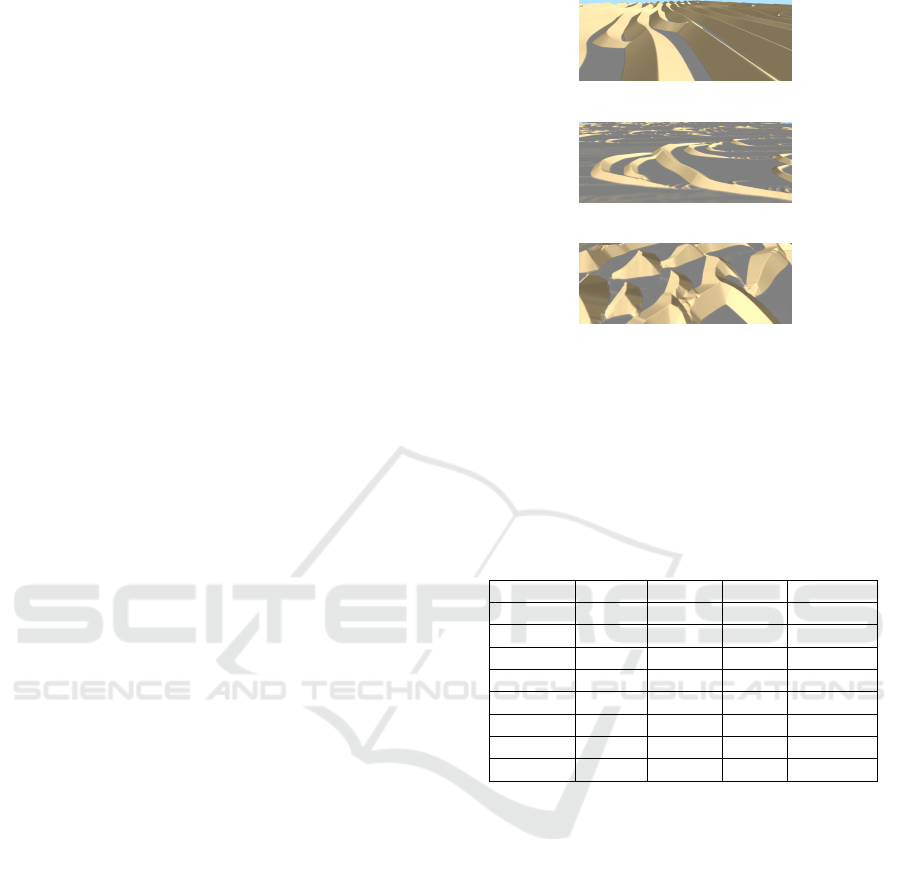
Figure 2 shows examples of different dune types gen-

erated by our method. Compared to Figure 4 in (Tay-

lor and Keyser, 2023), our results are noise-free, lead-

ing to a much clearer dune shape.

We evaluate the performance of our method on a

RTX 4080 GPU using the same two scenes as in Ta-

ble 1 (Scene A) and Table 2 (Scene B) in (Taylor and

Keyser, 2023). Results are summarized in Table 1.

Our method is 9× faster at best and 1.5× faster than

the previous GPU implementation at worst, where the

speedup is larger with lower resolutions. Note that

we do not know exactly how many avalanche iter-

(a) Transverse.

(b) Barchan.

Figure 2: Different dune types generated with our method.

Compared to Figure 4 of (Taylor and Keyser, 2023), we

achieve better detail with our noise-free implementation.

ations were done in the previous work, so an exact

comparison is tricky because avalanching is the most

time-intensive portion of the algorithm.

Table 1: Simulation of 1000 steps at different resolutions in

barchan (A) and transverse (B) dune environments.

Scene l Taylor Ours Speedup

A, 512 2m 4.2s 0.46s 9.1x

B, 512 2m 4.2s 0.51s 8.2x

A, 1024 1m 8.3s 1s 8.3x

B, 1024 1m 8.3s 1.2s 6.9x

A, 2048 0.5m 24.8s 5.9s 4.2x

B, 2048 0.5m 24.8s 7.4s 3.4x

A, 4096 0.25m 97.2s 47.9s 2x

B, 4096 0.25m 121.4s 81.8s 1.5x

We made sure to use enough avalanching itera-

tions to properly converge in all situations and detail

this in Table 2, along with the time spent on the two

most signiﬁcant parts of the algorithm - wind warp-

ing and avalanching. We also detail the percentage

of time spent on avalanching, which grows from 35%

at low resolutions to up to 85% at higher resolutions

and higher sand availability. In general, avalanching

performance grows not only with resolution, but also

with the inverse of the detail resolution. If cell width

is halved, dune cross-sections span twice as many

cells, which means roughly twice as many iterations

are needed to converge. This leads to a theoretical 8×

growth in our scenes as we double vertical and hori-

zontal resolution while halving cell width l.

At 1024 × 1024 resolution, a simulation step only

takes about 1ms with our method. This means that this

resolution could feasibly be simulated in real-time in

games during gameplay, where the time budget is ex-

Real-Time Desertscapes Simulation with CUDA

θ = 45

◦

θ = 105

◦

θ = 150

◦

θ = 45

◦

θ = 105

◦

θ = 150

◦

φ = 100%

φ = 22%

φ = 64%

φ = 7%

Figure 3: Dune formation under a bidirectional wind scheme with varying sand availability φ. θ is the angle between the two

wind vectors. The left half of each image has reptation disabled, while the right half uses a high reptation strength. Results

are very smiliar to Figure 3 in (L

u et al., 2018) and match more closely than (Taylor and Keyser, 2023) in many cases.

Table 2: Average time spent on wind warping and avalanch-

ing in each simulation step and the percentage of time

spent on avalanching. The last column shows how many

avalanching iterations were done per step.

Scene WW Aval. %Aval. Iters.

A, 512 0.1ms 0.16ms 35% 13

B, 512 0.1ms 0.19ms 37% 15

A, 1024 0.2ms 0.57ms 57% 25

B, 1024 0.2ms 0.76ms 63% 31

A, 2048 1ms 3.9ms 66% 50

B, 2048 1ms 5.5ms 74% 62

A, 4096 6.9ms 34.9ms 73% 100

B, 4096 6.9ms 69.4ms 85% 125

tremely limited. At higher resolutions such as 2048 ×

2048 we would need to simplify the method. With-

out wind warping and with low wind speed such that

15 avalanching iterations are enough, we can reach

2.3ms per time step. If we further split the algorithm

over two frames, we can reduce this to 1.4ms which

is the time spent on just avalanching. To support

the full method at this resolution we would have to

split the avalanching iterations over multiple frames

as well, in which case a 1ms target is possible even

with wind warping. Our method is thus suitable for

use during gameplay at high resolutions. The main

challenge would be collision handling, since eleva-

tion values exist on the GPU, but collision is usually

done on CPU.

We evaluate our method against an established

ofﬂine method in a bidirectional wind scheme with

strength ratio R = 2 at different wind angles θ and

sand availability φ in the same way as the previous

work (Taylor and Keyser, 2023; L

u et al., 2018). Re-

sults are shown in Figure 3. We evaluated each set of

parameters using no reptation as well as using a high

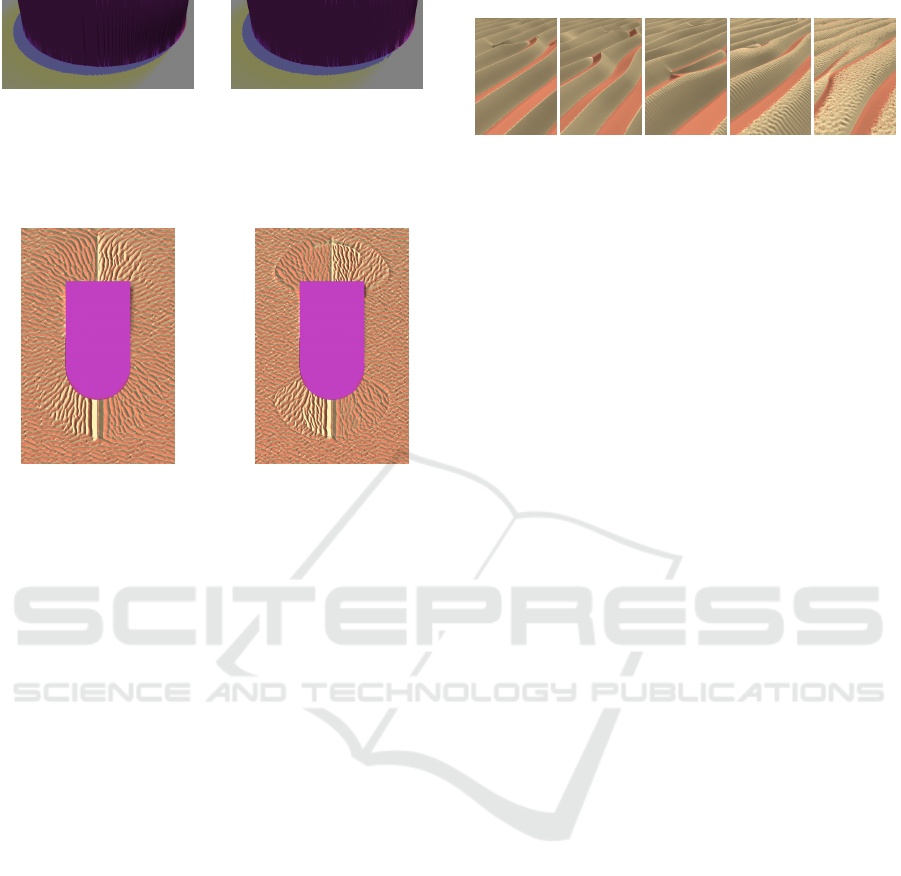
(a) Without reptation. (b) With reptation.

Figure 4: Example of an echo dune in a wind tunnel similar

to Figure 8 in (Taylor and Keyser, 2023) at a 2048 × 512

resolution. The aliased nature of the obstacle is visible in

the dune, which is smoothed using our reptation algorithm.

reptation strength. Compared to the previous work,

our results at φ = 22%,θ ≥ 105

◦

match the reference

more closely, where we can reproduce the long tails

that form on dunes. Additionally, our reptation algo-

rithm manages to generate dune shapes that are much

more consistent with the reference, reproducing the

rounder dune shapes and matching the width of the

windward side of the dune in relation to the leeward

side more closely. At φ = 7%, θ ≥ 105

◦

, we struggle

to reproduce the results of the ofﬂine method, just like

the previous work. While we do generate long linear

dunes and small detached barchans, they do not merge

to a single dune. It is possible that this is just a matter

of initial conditions, as we iteratively place small cir-

cles of sand at random positions until the target sand

availability is reached.

Figure 4 shows a scene similar to the wind tun-

nel experiments in (Taylor and Keyser, 2023) using

a round obstacle. Unlike previous work, we support

non-square resolutions, removing a signiﬁcant limi-

tation for such scenes. With reptation disabled, the

aliased nature of the obstacle is visible in our dune

GRAPP 2024 - 19th International Conference on Computer Graphics Theory and Applications

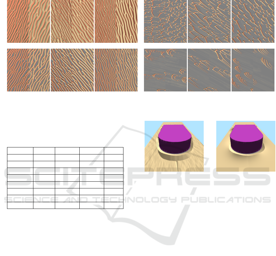
(a) Bilinear interpolation. (b) Nearest neighbor.

Figure 5: Sticky (yellow) and erosion (blue) cells around

an obstacle at a grazing wind angle. Using bilinear inter-

polation in cliff cell generation removes holes in the cell

classiﬁcation.

(a) Bilinear interpolation. (b) Nearest neighbor.

Figure 6: A scene with strong wind warping around an ob-

stacle. Using bilinear interpolation in advection and wind

shadow calculation, the dunes smoothly follow the wind

ﬁeld, while nearest neighbor leads to visible discontinuities.

shape. This wasn’t visible in the previous work, but

we note that this may have been hidden by the noise

of their method as well as the smaller size of the echo

dune in their example. If we enable our new repta-

tion method, the dune shape is smoothed signiﬁcantly

and the artifacts are no longer visible. In Figure 5

we show the same obstacle, visualizing the generated

sticky and erosion cells at a wind angle of 70

◦

. With

the original cliff cell generation that uses the near-

est upwind neighbor cell, some cells at grazing an-

gles aren’t classiﬁed properly. Our method with bilin-

ear interpolation in cliff cell generation removes these

problems.

Bilinear interpolation during advection and wind

shadow calculation also leads to large improvements

over nearest neighbor. At low wind speeds, nearest

neighbor would either generate no movement at all,

or a much faster movement than intended, which is

solved with bilinear interpolation. Figure 6 shows an

example scene with strong wind warping around an

obstacle. With our method, dune orientation smoothly

follows the warped wind ﬁeld. With the previous

nearest neighbor implementation, clear discontinu-

ities and artifacts are visible.

Using curved mode in wind shadow calculation

had a negligible impact in the scenes we tested, pro-

viding little beneﬁt for its computational cost. Hence,

we used the simpler linear mode for all results pre-

= 0 k

= 1 k

= 5 k

= 10 k

= 20

Figure 7: Transverse dunes at different reptation

strengths k

sented in this paper which is also what was used in

previous work.

Figure 7 shows a transverse dune environment at

different reptation strengths k

. At k

= 1, our rep-

tation method has a smoothing effect which can im-

prove results signiﬁcantly (see also Figure 4). With

higher reptation strengths the dune shape is changed

signiﬁcantly, where the windward side grows wider

with reduced angle, while the leeward side shrinks.

As described earlier, this type of dune shape is more

consistent with simulation results using ofﬂine meth-

ods established in geomorphology (see Figure 3).

However, high reptation strengths also introduce rip-

ples parallel to the wind direction on the windward

side of dunes which oscillate with each simulation

step. At even higher strengths, the linear ripples re-

cede and are replaced by circular ripples. While these

ripples look visually interesting and match sand rip-

ples, they are oriented the wrong way and the oscilla-

tions make this unsuitable in animation.

We evaluate our new sand distribution scheme for

avalanching against the previous method in (Taylor

and Keyser, 2023). Figure 9 shows a 100 × 100 cell

column of height 400m after 250 steps of 50 avalanch-

ing iterations each. Using our method with k

= 1, the

sand column is almost fully stabilized and the artifacts

are already barely visible. If we use k

= 0.5 for ev-

ery 10th iteration as well as the last 5 iterations in each

simulation step, convergence is slightly slower at the

beneﬁt of further reducing artifacts. Note that all ar-

tifacts are gone once convergence is reached, so this

is not really necessary if enough iterations are used

at runtime. (Taylor and Keyser, 2023) used k

= 0.25

with their algorithm, but we also include k

= 0.5 in

our comparison as it behaved stable in our implemen-

tation, likely because we are using ﬂoats for elevation

instead of integers. At k

= 0.5, their method is still

further from convergence than both of our examples,

while exhibiting stronger artifacts. Using k

= 0.25,

convergence is very slow. Our method needs signiﬁ-

cantly fewer steps to reach convergence. We suspect

that our performance measurements in Table 1 would

compare even better if we knew the exact number of

iterations used in the previous work, which would al-

low us to exactly match the number of iterations to

Real-Time Desertscapes Simulation with CUDA

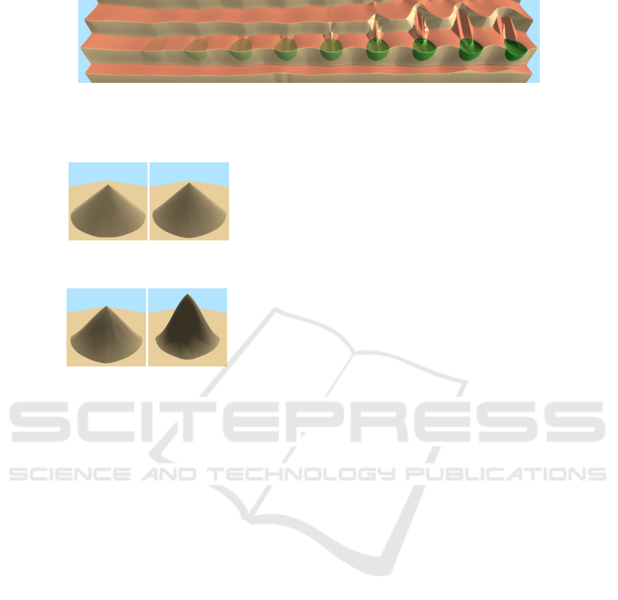
Figure 8: The impact of circular patches of vegetation (green) on transverse dunes. Dunes are moving upward in this image

and vegetation density of each patch increases from 0 to 1 (left to right). Vegetation signiﬁcantly alters sand transport and has

a large impact on dune morphology as it acts as a soft barrier in all sand transport calculations.

= 1 k

= {1,0.5}

(a) Ours.

= 0.5 k

= 0.25

(b) Taylor.

Figure 9: Comparison of our avalanching algorithm

with (Taylor and Keyser, 2023). The previous work

used k

= 0.25 but works stable at k

= 0.5 in our imple-

mentation. In our method, k

= {1, 0.5} means that every

10th iteration and the ﬁnal 5 iterations use the lower value.

reach the same level of convergence.

Lastly, all previous scenes were done with a veg-

etation density of 0, as we are comparing against re-

sults of previous work which did not include vegeta-

tion. Furthermore, our approach to vegetation is un-

changed from previous work. For completeness, Fig-

ure 8 shows the impact of patches with increasing

vegetation density in a transverse dune scenario. Veg-

etation alters the dune shape, leads to steeper slopes

and at higher densities, new dunes can form behind

vegetation.

6 CONCLUSION

In conclusion, our real-time GPU implementation fur-

ther improves on the performance of previous work.

The signiﬁcant increase in performance makes our

method viable during gameplay at a 1 − 2ms budget,

even at high resolutions such as 2048

, which was not

feasible in previous work.

Our method generates improved results compared

to previous work, producing smoother dune shapes

due to the removal of randomness and thus noise in

our algorithm. The bilinear interpolation shows sig-

niﬁcant improvements in wind warping scenarios as

well as wind angles that are misaligned with the cell

discretization and shows improvement in cell classi-

ﬁcation of echo dunes. We also show improvements

in the shape of dunes generated by our method, espe-

cially using our new reptation algorithm, producing

results that match the reference ofﬂine method more

closely overall. The support for non-square resolu-

tions makes our method more versatile than previous

work.

Like previous work, the main limitation is in res-

olution. All buffers and textures need to be avail-

able at the same time on the GPU, so we are limited

by VRAM. Performance currently scales increasingly

worse with higher resolutions due to memory band-

width.

For future work, in the short-term we would like to

extend the method to handle a bigger variety of land-

scapes. The simulation could be combined with a hy-

draulic erosion method such as (

St’ava et al., 2008).

In order to use our simulation to change landscapes

during gameplay, we need a reliable way to handle

dynamic objects. Static objects that affect the simula-

tion one-way are already possible using the bedrock

and object map, but dynamic objects such as play-

ers or vehicles need to be able to collide with the

terrain which currently exists as a heightmap on the

GPU, posing problems for physics engines. However,

one-way as well as two-way collision methods exist

for GPU-based ﬂuid simulations using heightmaps, so

this is possible.

In the medium term, we would like to further

improve reptation. The oscillating ripples that can

form at high strengths are a problem. Additionally,

we would like to see improvements to the vegetation

model, including two-way interactions. For example,

by introducing a water model, vegetation could dy-

namically grow and wither. Sand transport could be

enhanced to allow vegetation to be buried.

Long term, performance improvements are still

possible. The main focus should be avalanching as

it has the biggest performance impact. We made

attempts to speed up avalanching with a multigrid

GRAPP 2024 - 19th International Conference on Computer Graphics Theory and Applications

solver but were unable to achieve satisfying, artifact-

free results. The corresponding code can be found in

the supplementary material or on GitHub. Based on

our initial attempts, a multigrid solver could improve

performance by 2-8 times.

Lastly, while our focus was on performance with

realtime computer graphics in mind, increasing real-

ism of the method would be important for applica-

tions in geomorphology. A tiled simulation would en-

able simulating very large scale scenes on super com-

puters. Furthermore, we think that the simplistic wind

model is the reason why scenes with low sand avail-

ability do not behave as expected. A proper 3D wind

simulation may be able to solve some of these issues.

REFERENCES

Beakawi Al-Hashemi, H. M. and Baghabra Al-Amoudi,

O. S. (2018). A review on the angle of repose of gran-

ular materials. Powder Technology, 330:397–417.

Bene

s, B. and Roa, T. (2004). Simulating desert scenery.

WSCG ’2004: Short Communications: the 12-th In-

ternational Conference in Central Europe on Com-

puter Graphics, Visualization and Computer Vision

2004, pages 17–22.

Galin, E., Gu

erin, E., Peytavie, A., Cordonnier, G., Cani,

M.-P., Benes, B., and Gain, J. (2019). A review of

digital terrain modeling. Computer Graphics Forum,

38(2):553–577.

Gao, X., Narteau, C., Rozier, O., and Du Pont, S. C. (2015).

Phase diagrams of dune shape and orientation depend-

ing on sand availability. Scientiﬁc reports, 5(1):14677.

Kochanski, K., Defazio, G.-C., Green, E., Barnes, R.,

Downie, C., Rubin, A., and Rountree, B. (2019a).

Rescal-snow: Simulating snow dunes with cellular au-

tomata. Journal of Open Source Software, 4(42):1699.

Kochanski, K., Mohan, D., Horrall, J., Rountree, B., and

Abdulla, G. (2019b). Deep learning predictions of

sand dune migration. CoRR, abs/1912.10798.

Kri

stof, P., Bene

s, B., K

riv

anek, J., and

St’ava, O. (2009).

Hydraulic erosion using smoothed particle hydrody-

namics. Computer Graphics Forum, 28(2):219–228.

Lancaster, N. (2013). Geomorphology of desert dunes.

Routledge.

Livingstone, I. and Warren, A. (2019). Aeolian geomor-

phology: a new introduction.

u, P., Dong, Z., and Rozier, O. (2018). The combined

effect of sediment availability and wind regime on

the morphology of aeolian sand dunes. Journal of

Geophysical Research: Earth Surface, 123(11):2878–

2886.

Mandelbrot, B. B. and Van Ness, J. W. (1968). Fractional

brownian motions, fractional noises and applications.

SIAM Review, 10(4):422–437.

Mei, X., Decaudin, P., and Hu, B.-G. (2007). Fast hydraulic

erosion simulation and visualization on gpu. In 15th

Paciﬁc Conference on Computer Graphics and Appli-

cations (PG’07), pages 47–56.

Musgrave, F. K., Kolb, C. E., and Mace, R. S. (1989).

The synthesis and rendering of eroded fractal terrains.

In Proceedings of the 16th Annual Conference on

Computer Graphics and Interactive Techniques, SIG-

GRAPH ’89, page 41–50, New York, NY, USA. As-

sociation for Computing Machinery.

Nilles, A. M. and G

unther, L. (2023). Cuda

dune simulation. https://github.com/Clocktown/

CUDA-Dune-Simulation.

Paris, A. (2022). Desertscapes simulation. https://github.

com/aparis69/Desertscapes-Simulation/commit/

38298220d0182d97ff1f12e7f6aa8850fac1b52b.

Paris, A., Peytavie, A., Gu

erin, E., Argudo, O., and Galin,

E. (2019). Desertscape simulation. Computer Graph-

ics Forum, 38(7):47–55.

Rozier, O. and Narteau, C. (2014). A real-space cellular

automaton laboratory. Earth Surface Processes and

Landforms, 39(1):98–109.

Stam, J. (1999). Stable ﬂuids. In Proceedings of the 26th

Annual Conference on Computer Graphics and Inter-

active Techniques, SIGGRAPH ’99, page 121–128,

USA. ACM Press/Addison-Wesley Publishing Co.

St’ava, O., Bene

s, B., Brisbin, M., and K

riv

anek, J.

(2008). Interactive terrain modeling using hydraulic

erosion. In Proceedings of the 2008 acm sig-

graph/eurographics symposium on computer anima-

tion, pages 201–210.

Taylor, B. and Keyser, J. (2023). Real-time sand dune sim-

ulation. Proc. ACM Comput. Graph. Interact. Tech.,

6(1).

Tsoar, H. (1983). Wind tunnel modeling of echo and climb-

ing dunes. In Brookﬁeld, M. and Ahlbrandt, T., ed-

itors, Eolian Sediments and Processes, volume 38 of

Developments in Sedimentology, pages 247–259. El-

sevier.

Wang, N. and Hu, B.-G. (2009). Aeolian sand movement

and interacting with vegetation: A gpu based simula-

tion and visualization method. In 2009 Third Interna-

tional Symposium on Plant Growth Modeling, Simula-

tion, Visualization and Applications, pages 401–408.

Wang, N. and Hu, B.-G. (2012). Real-time simulation of

aeolian sand movement and sand ripple evolution: a

method based on the physics of blown sand. Journal

of Computer Science and Technology, 27(1):135–146.

Zhang, D., Narteau, C., and Rozier, O. (2010). Morphody-

namics of barchan and transverse dunes using a cel-

lular automaton model. Journal of Geophysical Re-

search: Earth Surface, 115(F3).

Real-Time Desertscapes Simulation with CUDA