ML-Tree and MRL-Tree: Combining Mass-Spring System, Rigid-Body

Dynamics and L-Systems to Model Physical Effects on Trees

See Min Lim

1 a

and Like Gobeawan

2 b

National University of Singapore, 21 Lower Kent Ridge Road, Singapore

Institute of High Performance Computing (IHPC), Agency for Science, Technology and Research (A*STAR),

1 Fusionopolis Way #16-16 Connexis, 138632, Singapore

Keywords:

Physically-Based Modeling, Tree Modeling, Root Modeling, L-Systems, MSS, RBD.

Abstract:

We apply physically-based modeling methods to a biological tree model for a hybrid model with a better

accuracy. Physical aspects of tree growth, such as wind, tropisms, gravity and soil resistance are modelled.

The hybrid model also includes the handling of boundary conditions such as momentum conservation and

switching between the L-System, Mass-Spring System (MSS) and Rigid-Body Dynamics (RBD) methods.

This paper demonstrates resulting models and their potential applications such as tree stress prediction.

1 INTRODUCTION

Trees and other greeneries are planted at urban areas

to provide shade and to reduce temperatures (Wong

et al., 2021). Along with that, they may cause safety

hazards due to uprooting and falling branches. They

can be managed through measures like tree health as-

sessment and tree pruning.

Given the increasing prominence of digital twin

cities (Ballouch et al., 2022) (Tao et al., 2022)

(Pomeroy, 2023), there are great potentials for digi-

tal twin trees through an automated large-scale tree

management system such as (Gobeawan et al., 2021a)

(Gobeawan et al., 2018) to consider biological growth

rules and mechanical responses to the environment.

Such digital twin trees can be utilised to predict tree

branch stress and uprooting.

2 RELATED WORK

Some existing L-System-based tree modelling tech-

niques (Gobeawan et al., 2021b) (Yi et al., 2018)

(Stava et al., 2014) focus on implementing tree

growth processes without accounting for the tree

tropisms, which are tree growth responses to environ-

ment stimuli. Accounting for such responses will al-

low for more accurate tree models in urban contexts of

https://orcid.org/0009-0008-0576-556X

https://orcid.org/0000-0001-6501-6394

intertwining environment components, hence a better

urban planning. (Moulton et al., 2020) and (H

adrich

et al., 2017) account for tree growth responses as me-

chanical responses by modelling tree stems as inex-

tensible elastic rods and particles, respectively. How-

ever, neither of them integrates the domain knowl-

edge of botanical growth processes such as branch-

ing patterns. (Jirasek et al., 2000) is similar, but it

is L-System-based (Prusinkiewicz and Lindenmayer,

1990) thus allowing for some biological considera-

tions. However it does not consider interactions be-

tween parent and child branches.

Our previous work (Lim and Gobeawan, 2023)

combines Mass-Spring System (MSS) and L-Systems

to generate biologically- and physically-plausible tree

models. This current work will provide crucial imple-

mentation details and results, as well as discuss new

work on root modeling and including Rigid-Body Dy-

namics (RBD).

3 METHODS

Our tree models were generated based on (Gobeawan

et al., 2021b) where stems were built by produc-

ing new node-and-internode pairs at the buds based

on L-System growth rules over time. During the

growth process, we concurrently built a MSS into our

tree models to model mechanical responses for our

ﬁrst model of Mass-Spring L-Systems (henceforth de-

220

Lim, S. and Gobeawan, L.

ML-Tree and MRL-Tree: Combining Mass-Spring System, Rigid-Body Dynamics and L-Systems to Model Physical Effects on Trees.

DOI: 10.5220/0012315200003660

Paper published under CC license (CC BY-NC-ND 4.0)

In Proceedings of the 19th International Joint Conference on Computer Vision, Imaging and Computer Graphics Theory and Applications (VISIGRAPP 2024) - Volume 1: GRAPP, HUCAPP

and IVAPP, pages 220-227

ISBN: 978-989-758-679-8; ISSN: 2184-4321

noted as ML-Tree). For our second Mass-Spring L-

Systems with RBD model (denoted as MRL-Tree),

we further added RBD to model older portions of the

tree.

With these models, we considered tropisms (pho-

totropism and gravitropism), weight of the tree nodes,

roots and soil resistance. Stress prediction and auto-

matic branch-breaking were also tested in the former

model.

Our images and models were generating using L-

Py and PlantGL (Boudon et al., 2012).

3.1 Mass-Spring L-System (ML-Tree)

When incorporating the MSS (Witkin et al., 2001)

onto the L-System layer, we consider the nodes to be

point masses while the internodes were springs. The

algorithm is described in the following pseudocode:

initialization;

for number of age timesteps do

tree grows for 1 unit of age by L-System

production rules;

for number of substeps do

calculate forces acting on each MSS

node;

calculate and update new position of

each node;

end

Algorithm 1: ML-Tree.

Firstly, we initialised expandable matrices to keep

track of nodal information and spring connection in-

formation. We also set the growth and physical vari-

ables (such as the trunk height and wind speed) to spe-

ciﬁc values or as functions. The tree then grows for

one unit of age by L-System production rules, where

one unit of age is the time needed to grow one node-

and-internode pair at each bud. This is the smallest

unit of growth possible in our model, chosen to min-

imise the time lag between the growth and the apply-

ing of forces. We then added the new node(s) grown,

their corresponding nodal information and the new

spring(s) information to the bookkeeping matrices.

Internal forces acting on each node (such as the spring

forces) are calculated based on the MSS model. Other

external forces acting on the nodes (such as gravity

and tropisms) are also calculated and added, and new

positions after the substep are found. This force and

position calculation is then repeated for the number

of substeps. This tree growth and force-and-position

calculation then repeats until the tree has reached its

speciﬁed age.

3.1.1 Conserving Momentum

In our model, the total and individual masses regu-

larly increases, hence the law of conservation of linear

momentum must be considered.

During the growth process, when a new node j is

grown, it shares the original linear momentum, m

of the node i which it grew from. Nodes i and j have

the same new velocity, v

t+δt

, since forces are not con-

sidered during this growth stage. To simplify calcu-

lations, we assume that new nodes are grown instan-

taneously at the start of the growth process, thus the

mass for the older node i at times t and t + δt are con-

sidered the same. We calculate the new velocities of

nodes i and j through Equation 1. m

t+δt

is the small-

est mass a new node can have in our model.

t+δt

= v

t+δt

+ m

t+δt

(1)

At the end of each age timestep, the mass of the

nodes are recalculated by multiplying the new volume

of their internodes with the wood density. The veloc-

ity of nodes are re-calculated by dividing the original

linear momentum with the new mass.

3.1.2 Spring Constants and Angle Springs

The spring constant of each spring are directly pro-

portional to the diameter d of the internode and in-

versely proportional to the internode’s rest length l

(Smith, 2010). The values of the spring constants

were roughly based on the spring constants of wood in

(Russell and Hunt, 2009). Nodes which have reached

a certain wooden age are considered to be woody and

will have a stiffer base spring constant k

k =

(2)

Secondary (angle) springs were added between al-

ternate nodes to control angles, similar to (Van Haevre

et al., 2006). We used the same Equation 2 to ﬁnd the

secondary spring constants, and we did not differenti-

ate between the spring types for k

3.1.3 Implicit Method Equations

We used an implicit Euler method (or backward Eu-

ler) for integration in our MSS. We tested two equa-

tions to estimate ∆v

t+h

, Equation 3 (Kang et al.,

2001) and Equation 4 (Kang et al., 2000) (Mesit et al.,

2007).

is the sum of all forces acting on node i at

time t, and its unit vector is

ML-Tree and MRL-Tree: Combining Mass-Spring System, Rigid-Body Dynamics and L-Systems to Model Physical Effects on Trees

221

∆v

t+h

h+h

(i, j)∈E

i j

h/(m

( j,k)∈E

)

(i, j)∈E

i j

(3)

∆v

t+h

h + h

(i, j)∈E

i j

|∆v

+ h

(i, j)∈E

i j

(4)

These implicit methods required artiﬁcial damp-

ing for stability, which is given by Equation 5 in our

model.

damping

= c

k(m

+ m

)(v

− v

) (5)

It is chosen to be proportional to

k(m

+ m

)

to account for changing masses and spring constants

since we are modeling a growing tree. This coefﬁ-

cient is based on the formula for the critical damping

coefﬁcient, although we note that this Equation 5 is

not always able to achieve stability across all portions

of the tree.

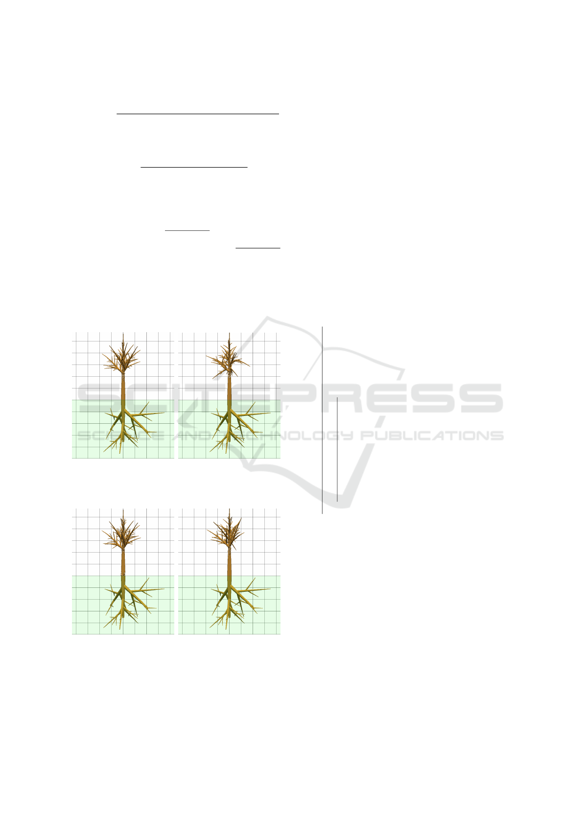
(a) Equation 3. (b) Equation 4.

Figure 1: Comparison of the ML-Tree model using Equa-

tion 3 and 4.

(a) Equation 3. (b) Equation 4.

Figure 2: Another comparison of the model using Equations

3 and 4.

Figure 1 attains a stable conﬁguration of damping

and spring constants for using Equation 3, and it is

compared with how Equation 4 perform for the same

set of variables. We tried to achieve the opposite sit-

uation in Figure 2, but we see that Equation 3 is sim-

ilarly realistic. Equation 3 tended to produce largely

realistic and stable models over a range of damping

and spring constants, while Equation 4 was only sta-

ble and realistic across a much narrower range.

3.2 Mass-Spring L-System with RBD

(MRL-Tree)

Our second model adds RBD (Baraff, 2001) (Peder-

sen, 2003) onto the existing MRL-Tree model. This

is described in algorithm 2. We used quaternions

(Betsch and Siebert, 2009) for the rotation and a 4-

th order Runge-Kutta (Pedersen, 2003) to solve the

differential equations.

initialization;

for number of age timesteps do

tree grows for 1 unit of age by L-System

production rules;

add nodes which have reached a speciﬁed

rigid age to the Rigid-Body (RB)

system;

for number of substeps do

calculate forces acting on each RB

node;

calculate and update new position of

each RB node;

calculate forces acting on each MSS

node;

calculate and update new position of

each MSS node;

end

Algorithm 2: MRL-Tree.

Our algorithm for this MRL-Tree model is similar

to that for the ﬁrst model, except that the forces and

positions of the RB nodes are considered ﬁrst before

that of the MSS nodes during each substep.

3.2.1 Handling Boundary Conditions for RBD

When a node reaches a speciﬁed age, it is considered

to have hardened and is added to the RB system. In

this subsection, t is at the end of the L-System stage

and t + δt is after the checking of age and assigna-

tion to the RB system, at the start of the ﬁrst substep.

Nodes j are these new RB nodes while nodes i are

existing RB nodes.

GRAPP 2024 - 19th International Conference on Computer Graphics Theory and Applications

222

The centre of mass of the RB system x and the

system’s linear momentum p can be directly calcu-

lated through Equations 6 and 7. M is the sum of

mass of the RB system. However since the RB sys-

tem is constantly increasing in size, the centre of mass

does not have a constant position relative to other po-

sitions in the RB system, therefore its original angular

momentum L

is not conserved. Hence, we hypothe-

sise that in Equation 8, an extra term Σ(x

t+δt

∆i

× m

)

should be added to account for any change in angu-

lar momentum due to the changing position of the

centre of mass. In Equation 8, x

t+δt

∆i

refers to the

relative position of node i at time t (or t + δt), to

the centre of mass at time t + δt; in other words,

t+δt

∆i

= x

− x

t+δt

Σm

+ Σm

t+δt

(6)

t+δt

= p

+ Σm

(7)

t+δt

≈L

+ Σ(x

t+δt

∆ j

× m

)

+ Σ(x

t+δt

∆i

× m

)

(8)

3.3 Gravity, Phototropism,

Gravitropism, Wind and Air

Viscosity

Gravity, F

, was calculated by multiplying the node’s

mass with g, the acceleration due to gravity on Earth.

Phototropism refers to the plant’s reorientation

towards light source and we modelled it with a

phototropism

which pulls the buds towards a speciﬁed

point of light (Moulton et al., 2020). Its magnitude is

a constant multiplied by the intensity of the light. The

light intensity is inversely proportional to the square

of the distance between the bud and the light source.

In future work, auxins should be considered to im-

prove accuracy (Zhou et al., 2017).

Gravitropism is the response of a plant to gravity.

Generally, the plant reorientates itself against the di-

rection of gravity and we modelled this F

gravitropism

based on the sine law method (Dumais, 2013). It is

applied on all nodes except the buds.

Wind was modelled using Equation 10, using a

general wind load formula. The constant in Equation

9 is only applicable for metric system of units, and

0.00256 should be used for the imperial system of

units. A is the area of the object for which we took the

cross-sectional area of the node, P is the wind pres-

sure and C

drag

is the drag coefﬁcient (set to 1 in our

model (Suzuki and Arikawa, 2010)).

P = 0.613|v

wind

(9)

wind

= (A × P ×C

drag

)

wind

(10)

Air viscosity was modelled based on Stokes’ Law

(Equation 11). In our model, η is the ﬂuid viscosity

(1.81 × 10

−5

for air), R is the radius of the node and v

is the velocity of the node.

drag

= 6πηRv (11)

3.4 Roots and Soil Resistance

There is currently a lack of research on root architec-

ture and modeling (Harahap et al., 2018)(Alani and

Lantini, 2020), especially those using a compatible L-

System method or for trees. This is partly due to the

difﬁculty in collecting underground root data, though

there has been recent advances in non-destructive root

testing methods (Alani and Lantini, 2020) (Atkinson

et al., 2019). Since any future biological modeling of

tree roots can be added retrospectively into our model,

we decided to focus on modeling the mechanical re-

actions of roots, and we modiﬁed the above-ground

tree growth to create a tentative model for the roots

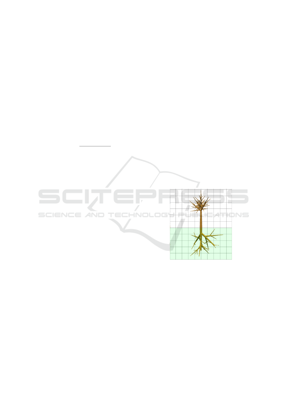
(Figure 3).

Figure 3: Tree model with roots, without mechanical forces.

To add soil resistance, we tested two models based

on (Pang et al., 2023) and (Imhoff et al., 2016). For

quantitative data on the soil (such as clay content or

organic matter content), we referred to (Rezaur et al.,

2003). Since the nodes underground are almost com-

pletely surrounded by the soil, we consider that the

roots can counter a net force in every direction. The

soil resistance calculated is considered to be the max-

imum soil resistance for the node.

The ﬁrst method uses Equation 12 (Pang et al.,

2023) and bulk density values from (Rezaur et al.,

2003). The poisson’s ratios used were estimated

based on the water content. γ is the soil density, µ

ML-Tree and MRL-Tree: Combining Mass-Spring System, Rigid-Body Dynamics and L-Systems to Model Physical Effects on Trees

223

is Poisson’s ratio, P

is the reaming pressure, r is the

radius of the cone and h is the penetration depth.

B = (

1000

)

× (0.5 − µ)

/2.8

max

| = (

10000

γ×9.8

1000000

π × r

)

× h × 100 × B

(12)

The second method uses Equation 14 from

(Imhoff et al., 2016) and soil data values from (Rezaur

et al., 2003). SR is the soil resistance to penetration

in MPa. clay represents the percentage clay content

while OM represents the percentage organic matter

content. θ is the volumetric water content, BD is the

bulk density of soil and A is the surface area. The co-

efﬁcients c

, c

, d

and e

are given in (Imhoff

et al., 2016).

lnSR =c

+ c

clay + c

+ (d

+ d

clay) ln θ + e

lnBD

(13)

max

| = 1000000 × SR × A (14)

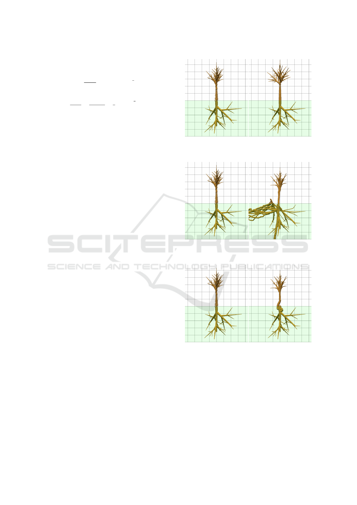
Figures 4, 5 and 6 show both methods using soil

data from three different locations (Yishun, Mandai

and NTU) in Singapore, with only gravity applied.

We notice some instability in almost all the cases,

which could be due to a number of reasons. Firstly,

our model is not an accurate representation of root

structure as discussed above. Secondly, it does not

consider soil penetration during root growth, includ-

ing any changes to the root model and soil proﬁle as a

result. Furthermore, our model also does not include

collision detection as this would be too computation-

ally costly.

Overall, we consider the second method to be

more suitable. This is because it allows direct alter-

ation in the soil type since the percentages of clay,

water, bulk density, organic matter are all considered.

We also notice that for the Yishun tree models, the

second method is mostly stable, unlike for the ﬁrst

method. Both models are unstable for the Mandai and

NTU models.

3.5 Stress Prediction and Automatic

Branch-Breaking

Given that our ML-Tree model keeps track of forces

and nodal information, we can calculate and predict

the stress on each node. This is shown in Figure

7. The colour varies on a logarithmic scale; darker

blue indicates more stress and the lightest blue ap-

pears nearly white.

(a) Method 1. (b) Method 2.

Figure 4: Comparison using Yishun’s environment.

(a) Method 1. (b) Method 2.

Figure 5: Comparison using Mandai’s environment.

(a) Method 1. (b) Method 2.

Figure 6: Comparison using NTU’s environment.

Based on the stress, we can also set an automatic

branch breaking limit. This can help improve our

digital twin tree model accuracy by automatically re-

moving branches experiencing a high level of stress,

which would have naturally fallen.

From Figure 7, the areas under most stress (e.g.

when the branches curve downwards signiﬁcantly),

are darkly coloured as expected. However, from Fig-

ure 7, the sudden changes in colour of neighbouring

GRAPP 2024 - 19th International Conference on Computer Graphics Theory and Applications

224

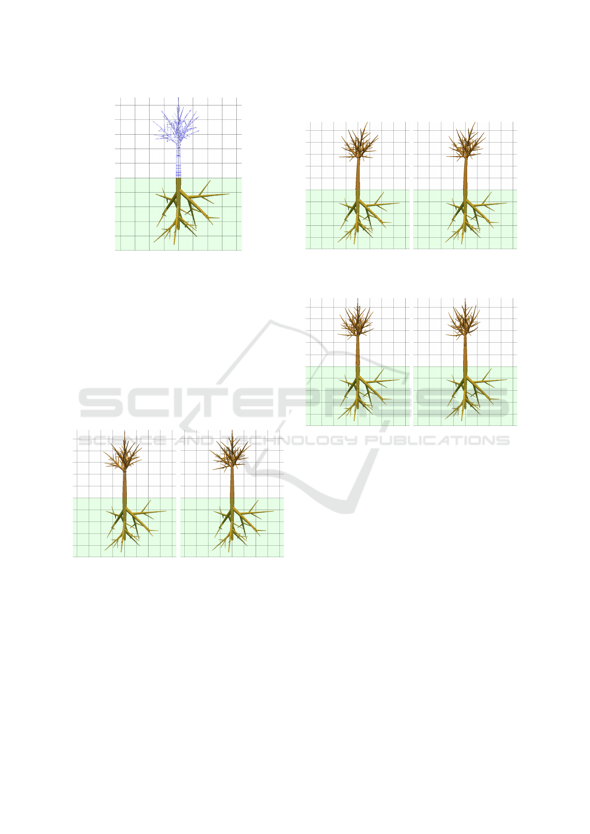
Figure 7: Tree model coloured based on stress.

internodes suggests that our models have difﬁculty

reaching a ﬁnal equilibrium state.

4 RESULTS AND DISCUSSION

In this section, we compared the two models. Our ex-

amples were generated based on a 25 year-old Hopea

odorata tree. The age when nodes become rigid was

set to 3 years for the MRL-Tree model.

4.1 Gravity

(a) ML-Tree. (b) MRL-Tree.

Figure 8: Comparison of gravity effects on the two models.

We noticed from Figure 8 that MRL-Tree model was

signiﬁcantly more rigid than our ML-Tree model.

4.2 Tropisms

Figure 9 shows a comparison of the two models with

phototropism applied, and the trees can be seen bend-

ing towards the light source on the right. Figure 10

has gravitropism applied, and the tree branches are

seen bending upwards as expected. We noticed that

the two models produced essentially identical results

in both cases.

(a) ML-Tree. (b) MRL-Tree.

Figure 9: Comparison of phototropism effects on the two

models.

(a) ML-Tree. (b) MRL-Tree.

Figure 10: Comparison of gravitropism effects on the two

models.

4.3 Wind

We also tested adding wind to our model, as shown in

Figure 11. However, for our ML-Tree model, the elas-

ticity and difﬁculty in propagation of forces causes

our tree to collapse. Since we did not implement the

tree collapse processes, Figure 11a appears unstable.

This is not the case in our MRL-Tree model, which

compels the forces to be completely propagated.

4.4 Comparison of the Two Models

From the model with wind applied (Figure 11), we

see that the soil resistance has difﬁculty keeping the

ML-Tree upright, causing the instability. This is be-

cause the ML-Tree model has difﬁculty propagating

the forces throughout the system within its 50 sub-

steps per L-System time-step, resulting in the model

appearing to be too elastic. Meanwhile the MRL-Tree

calculates the displacement effects for the whole RB

system together, compelling the forces to be propa-

ML-Tree and MRL-Tree: Combining Mass-Spring System, Rigid-Body Dynamics and L-Systems to Model Physical Effects on Trees

225

(a) ML-Tree (unstable). (b) MRL-Tree.

Figure 11: Comparison of wind effects on the two models.

gated, and therefore it is more stable and realistic.

However, this second model also faces stiffness

issues as seen from the case with gravity (Figure 8).

Furthermore, stress prediction and automatic branch

breaking, as they are currently implemented, will not

work with this second model since the RB nodes are

not considered individually.

5 CONCLUSION

We have demonstrated the feasibility of applying

physically-based methods to biological tree models

to attain two plausible models which can predict cru-

cial tree management information such as the relative

amounts of stress acting on each node. Our mod-

els can be scaled to include other environmental and

growth factors or to improve the current methods, as

long as these factors can be modelled as forces. We

also tested and compared varying methods of model-

ing soil resistance, of implicit integration and of pre-

dicting branch breaking possibility. In addition, we

also detailed the methods we used to handle bound-

ary conditions for both the ML-Tree model and the

MRL-Tree model. Our models are largely built us-

ing existing real-life data and physical laws of nature,

therefore they have the potential to be deployed for

tree management, with integration with a large-scale

tree-management system in a digital twin city.

However, our models currently suffer from stabil-

ity issues. Furthermore, for the total duration of sub-

steps and age timesteps to be equal, the substeps of

the MSS will need be very large, or the model will be

very computationally costly. More work can be done

to further improve stability and accuracy or create a

more accurate model to replace the tentative mod-

els currently used for roots. Other methods for solv-

ing ordinary differential equations can be explored to

improve stability. The models can also beneﬁt from

modeling more physical aspects to improve accuracy,

such as incorporating a collision detection system be-

tween the nodes of the model. For further model vali-

dation, a parameter ﬁtting method such as the method

detailed in (Gobeawan et al., 2021b) can be applied.

Beyond the context of plant modeling, we note

that our work in combining L-Systems, MSS and

RBD could also have applications in modeling other

objects such as bones and soft tissues (Golec, 2018),

medical procedures (Nakao and Minato, 2010) and

sound (Cahill, 2009).

ACKNOWLEDGEMENTS

This research/project is supported by the National

Research Foundation, Singapore under its Industry

Alignment Fund – Pre-positioning (IAF-PP) Funding

Initiative. Any opinions, ﬁndings and conclusions or

recommendations expressed in this material are those

of the authors and do not reﬂect the views of National

Research Foundation, Singapore.

REFERENCES

Alani, A. M. and Lantini, L. (2020). Recent advances in tree

root mapping and assessment using non-destructive

testing methods: a focus on ground penetrating radar.

Surveys in Geophysics, 41:605–646.

Atkinson, J. A., Pound, M. P., Bennett, M. J., and Wells,

D. M. (2019). Uncovering the hidden half of plants us-

ing new advances in root phenotyping. Current opin-

ion in biotechnology, 55:1–8.

Ballouch, Z., Hajji, R., Poux, F., Kharroubi, A., and Billen,

R. (2022). A prior level fusion approach for the se-

mantic segmentation of 3d point clouds using deep

learning. Remote Sensing, 14(14):3415.

Baraff, D. (2001). Physically based modeling: Rigid body

simulation. SIGGRAPH Course Notes, ACM SIG-

GRAPH, 2(1):2–1.

Betsch, P. and Siebert, R. (2009). Rigid body dynamics

in terms of quaternions: Hamiltonian formulation and

conserving numerical integration. International jour-

nal for numerical methods in engineering, 79(4):444–

473.

Boudon, F., Pradal, C., Cokelaer, T., Prusinkiewicz, P.,

and Godin, C. (2012). L-py: an l-system simulation

framework for modeling plant architecture develop-

ment based on a dynamic language. Frontiers in plant

science, 3:76.

Cahill, B. (2009). Physically based sound synthesis for in-

teractive applications. Master’s thesis, University of

Dublin, Trinity College.

Dumais, J. (2013). Beyond the sine law of plant gravit-

ropism. Proceedings of the National Academy of Sci-

ences, 110(2):391–392.

GRAPP 2024 - 19th International Conference on Computer Graphics Theory and Applications

226

Gobeawan, L., Lin, E., Tandon, A., Yee, A., Khoo, V., Teo,

S., Yi, S., Lim, C., Wong, S., Wise, D., et al. (2018).

Modeling trees for virtual singapore: From data acqui-

sition to citygml models. The International Archives

of the Photogrammetry, Remote Sensing and Spatial

Information Sciences, 42:55–62.

Gobeawan, L., Lin, S., Liu, X., Wong, S., Lim, C., Gaw, Y.,

Wong, N., Tan, P., Tan, C., and He, Y. (2021a). Ifc-

centric vegetation modelling for bim. ISPRS Annals

of the Photogrammetry, Remote Sensing and Spatial

Information Sciences, 8:91–98.

Gobeawan, L., Wise, D. J., Wong, S. T., Yee, A. T., Lim,

C. W., and Su, Y. (2021b). Tree species modelling

for digital twin cities. Transactions on Computational

Science XXXVIII, pages 17–35.

Golec, K. (2018). Hybrid 3D mass spring system for soft

tissue simulation. PhD thesis, Universit

e de Lyon.

adrich, T., Benes, B., Deussen, O., and Pirk, S. (2017).

Interactive modeling and authoring of climbing plants.

In Computer Graphics Forum, volume 36, pages 49–

61. Wiley Online Library.

Harahap, N., Siregar, I., and Dwiyanti, F. (2018). Root

architecture and its relation with the growth char-

acteristics of three planted shorea species (diptero-

carpaceae). In IOP Conference Series: Earth and En-

vironmental Science, volume 203, page 012016. IOP

Publishing.

Imhoff, S., Pires da Silva, A., Ghiberto, P. J., Tormena,

C. A., Pilatti, M. A., and Libardi, P. L. (2016).

Physical quality indicators and mechanical behav-

ior of agricultural soils of argentina. PLoS One,

11(4):e0153827.

Jirasek, C., Prusinkiewicz, P., and Moulia, B. (2000). Inte-

grating biomechanics into developmental plant mod-

els expressed using l-systems. Plant biomechanics,

pages 615–624.

Kang, Y.-M., Choi, J.-H., Cho, H.-G., and Lee, D.-H.

(2001). An efﬁcient animation of wrinkled cloth with

approximate implicit integration. The Visual Com-

puter, 17:147–157.

Kang, Y.-M., Choi, J.-H., Cho, H.-G., and Park, C.-J.

(2000). Fast and stable animation of cloth with an

approximated implicit method. In Proceedings Com-

puter Graphics International 2000, pages 247–255.

IEEE.

Lim, S. M. and Gobeawan, L. (2023). Hybrid mass-spring

l-system for modelling tree interactions with envi-

ronment. In Chen, T.-W. C., Fricke, A., Kahlen,

K., and St

utzel, H., editors, Book of Abstracts of

the 10th International Conference on Functional-

Structural Plant Models: FSPM2023, 27- 31 March

2023, pages 102–103.

Mesit, J., Guha, R. K., and Chaudhry, S. (2007). 3d soft

body simulation using mass-spring system with inter-

nal pressure force and simpliﬁed implicit integration.

J. Comput., 2(8):34–43.

Moulton, D. E., Oliveri, H., and Goriely, A. (2020). Mul-

tiscale integration of environmental stimuli in plant

tropism produces complex behaviors. Proceedings of

the National Academy of Sciences, 117(51):32226–

32237.

Nakao, M. and Minato, K. (2010). Physics-based inter-

active volume manipulation for sharing surgical pro-

cess. IEEE Transactions on Information Technology

in Biomedicine, 14(3):809–816.

Pang, J., Lin, X., Zhang, X., Ji, J., and Geng, L. (2023).

Modelling and analysis of penetration resistance of

probes in cultivated soils. PloS one, 18(1):e0280525.

Pedersen, S. W. (2003). Simulation of rigid body dynamics.

Master’s thesis.

Pomeroy, J. (2023). Hardware, Software, Heartware: Dig-

ital Twinning for More Sustainable Built Environ-

ments. Taylor & Francis.

Prusinkiewicz, P. and Lindenmayer, A. (1990). The Algo-

rithm Beauty of Plants. Springer.

Rezaur, R., Rahardjo, H., Leong, E., and Lee, T. (2003).

Hydrologic behavior of residual soil slopes in singa-

pore. Journal of Hydrologic Engineering, 8(3):133–

144.

Russell, D. and Hunt, L. (2009). Spring constants

for hockey sticks. The Physics Teacher (sub-

mitted draft). Retrieved from: www. acs. psu.

edu/drussell/publications/russell-hunt-tpt-formatted.

pdf (Accessed 17 January 2014).

Smith, J. O. (2010). Physical audio signal processing: For

virtual musical instruments and audio effects. W3K

Publishing.

Stava, O., Pirk, S., Kratt, J., Chen, B., M

ech, R., Deussen,

O., and Benes, B. (2014). Inverse procedural mod-

elling of trees. In Computer Graphics Forum, vol-

ume 33, pages 118–131. Wiley Online Library.

Suzuki, T. and Arikawa, T. (2010). Numerical analysis of

bulk drag coefﬁcient in dense vegetation by immersed

boundary method. In Proc. of the 32nd Conference on

Coastal Engineering.

Tao, F., Xiao, B., Qi, Q., Cheng, J., and Ji, P. (2022). Digital

twin modeling. Journal of Manufacturing Systems,

64:372–389.

Van Haevre, W., Di Fiore, F., and Van Reeth, F. (2006).

Physically-based driven tree animations. In NPH,

pages 75–82.

Witkin, A., Baraff, D., and Kass, M. (2001). Physically

based modeling. ACM SIGGRAPH Course Notes, 25.

Wong, N. H., Tan, C. L., Kolokotsa, D. D., and Takebayashi,

H. (2021). Greenery as a mitigation and adaptation

strategy to urban heat. Nature Reviews Earth & Envi-

ronment, 2(3):166–181.

Yi, L., Li, H., Guo, J., Deussen, O., and Zhang, X. (2018).

Tree growth modelling constrained by growth equa-

tions. In Computer Graphics Forum, volume 37,

pages 239–253. Wiley Online Library.

Zhou, Y., Wang, Y., Chen, X., Zhang, L., and Wu, K.

(2017). A novel path planning algorithm based on

plant growth mechanism. Soft Computing, 21:435–

445.

ML-Tree and MRL-Tree: Combining Mass-Spring System, Rigid-Body Dynamics and L-Systems to Model Physical Effects on Trees

227