Improvement of Tensor Representation Label in Image Recognition:

Evaluation on Selection, Complexity and Size

Shinji Niihara

1,2

and Minoru Mori

Faculty of Information Technology, Kanagawa Institute of Technology, Atsugi-shi, Kanagawa, Japan

SHARP Corporation, Sakai-shi, Osaka, Japan

Keywords: Deep Neural Network, Image Recognition, Label, Tensor Representation, Adversarial Examples.

Abstract: One-hot vectors representing correct/incorrect answer classes as {1/0} are usually used as labels for

classification problems in Deep Neural Networks. On the other hand, a method using a tensor consisting of

speech spectrograms of class names as labels has been proposed and reported to improve resistance to

Adversarial Examples. However, effective representations for tensor-based labels have not been sufficiently

studied. In this paper, we evaluate the effects of selections of image, complexity, and tensor size expansion

on the tensor representation labels. Evaluation experiments using several databases and DNN models show

that higher accuracies and tolerances can be achieved by improving tensor representations.

1 INTRODUCTION

Since high recognition accuracies in the image

recognition were achieved on AlexNet (Krizhevsky,

2012), Deep Neural Networks (DNNs) have been

used not only for image recognition but also for

understanding various media. When used for

classification problems, a one-hot vector is usually

used as a class label for each data with the correct

answer class set to 1 and the incorrect answer class

set to 0. In recent years, several methods of making

various improvements of the one-hot vector have

been proposed for generalizing DNNs. Label

smoothing (Szegedy, 2016), in which labels are

smoothed with a small amount of noise, has been

reported to improve recognition accuracies. Also,

Knowledge Distillation (Hinton, 2015) generalizes a

small DNN by using the output of a larger DNN as

the correct label. Knowledge Distillation can be

positioned as a kind of label smoothing from a

viewpoint of adjustment of the one-hot vector.

On the other hand, a different approach has been

proposed in (Chen, 2021). Their method trains the

output of a DNN to be close to image labels of each

class from images by setting 2D images consisting of

the speech spectrogram of each class name. In the

labelling of tensors consisting of these images,

recognition accuracies for ordinary images are

comparable to that using one-hot vectors, but the

improvement of robustness to Adversarial Examples

(AEs) has been reported (Szegedy, 14). However,

little sufficient understanding and evaluation of

properties of tensor representation labels exist. In this

paper, we extend the tensor representation of labels.

Specifically, we propose and evaluate extensions to

image selection as a base of tensor, its value range, its

complexity, and sizes of tensors.

2 RELATED WORKS

In this section we describe conventional methods

about the improvement on label representation in

DNNs.

2.1 Label Smoothing

Label smoothing (Szegedy, 2016) is a smoothing

technique that adds a small amount of noise to 0 of

incorrect classes in the one-hot vector. Specifically,

subtracting a small value of ε from 1 in the correct

class, and distributing a value obtained by dividing ε

by the number of classes to all the classes. This allows

smoothing the output of the softmax function used as

the loss function and the regularization effect on the

weight parameters (Lukasik, 2020). Therefore,

overfitting tends to be suppressed and generalization

performance is often improved.

232

Niihara, S. and Mori, M.

Improvement of Tensor Representation Label in Image Recognition: Evaluation on Selection, Complexity and Size.

DOI: 10.5220/0012313700003654

Paper published under CC license (CC BY-NC-ND 4.0)

In Proceedings of the 13th International Conference on Pattern Recognition Applications and Methods (ICPRAM 2024), pages 232-239

ISBN: 978-989-758-684-2; ISSN: 2184-4313

Hinton et al. have proposed Knowledge

Distillation (Hinton, 2015), which improves the

generalization performance of small DNN models. In

this technique, a small DNN model adjusts weight

parameters using not errors between predictions of

the small DNN model and one-hot vectors of the

correct labels, but errors between predictions of the

small DNN model and that of large and high-

performance trained DNN models during the training

process. Here, treating the predictions of the large-

scale model as labels for the training data can be

regarded as a kind of label smoothing techniques.

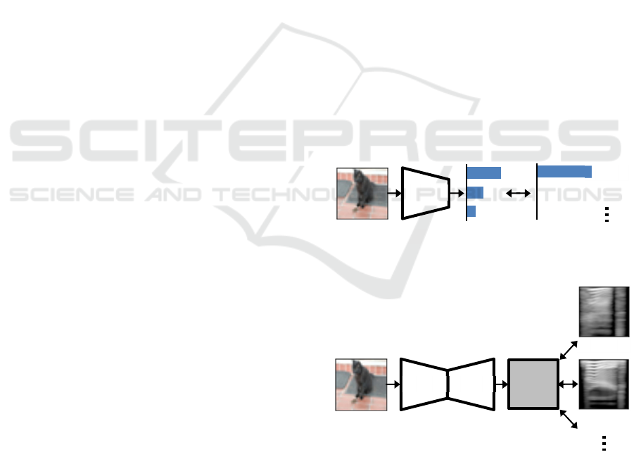
2.2 Tensor Representation

On the other hand, as a completely different

approach, a tensor as a 2-dimensional image based on

a speech spectrogram of each class label name is set

as the class label (Chen, 2021). The distance between

the tensor-based output of a DNN model and a tensor

as the 2-dimensional image of the correct label is used

for learning and inference. Figure 1 shows overviews

of a conventional process using a one-hot vector label

and their process using a tensor label based on a

speech spectrogram. In the process of (Chen, 2021),

a DNN model generates and outputs a tensor

consisting of a 2-dimensional vector obtained by the

deconvolution from the feature vector after the

convolution process. Their evaluation experiments

have confirmed that the recognition accuracy for

ordinary images is not so different from that obtained

using the one-hot vector, but the tolerance against

AEs (Goodfellow, 2015, Kurakin, 2017) is improved.

They also have reported that the increase of the

complexity of the speech spectrogram caused by

randomly switching the spectrogram among

frequencies, improves recognition accuracies.

3 PROPOSED METHOD

3.1 Our Approach

(Chen, 2021) mainly used a tensor consisting a two-

dimensional vector based on the speech spectrogram

for each class label. However, the validity of the

speech spectrograms mentioned above as a class label

has not been verified in any way. Several topics such

as a kind of image used, complexity, size of tensor,

and value range are also not sufficiently validated.

In this paper we seek to improve the tensor

representation label consisting a multidimensional

vector like an image from several perspectives. First,

we consider a selection of an image as a reference.

One is to select an image from training data itself and

the other uses a mean image obtained by averaging

training data for each class. As for the complexity of

the images, we add gaussian noise to reference

images and apply block ciphers to each reference

image. We also examine the expansion of the tensor

size and the number of channels to 3 channels (RGB).

Details of our proposed approach are described

below.

3.2 Tensor Representation Label

3.2.1 Image Selection

First, we consider the use of an image sampled from

the training data as a reference image to be set as a

label. If the output of the DNN is positioned as an

image reconstruction problem, sampling an image

from the training data and setting it a reference seem

to be reasonable. In this paper, we set labels as images

sampled from the training data for each class or the

averaged image of each class from the training data.

Figure 2 shows sampled images as tensor

representation labels from CIFAR10 (Krizhevsky,

2009), and examples of labels based on the mean

image for each class (each label of images is

“airplane”, “automobile”, “bird”, “cat”, and “deer”

from left to right in Figure 2, 3, 4 and 5).

(a) One-hot vector representation

(b) Tensor representation

Figure 1: Overviews of inference process using label of

one-hot vector and tensor representation labels.

Conv

DNNInput Output

Cat

Bir

One-hot vector

Label

Out

Conv Deconv

DNN

Bir

Cat

Tensor Label

Improvement of Tensor Representation Label in Image Recognition: Evaluation on Selection, Complexity and Size

233

3.2.2 Image Complexity

Next, we examine the complexity of images used as

tensor representation labels, since the study in (Chen,

2021) suggests that the entropy of images may affect

classification accuracies. In this paper, we adopted

two ways of increasing image complexity. One is the

addition of noise and the other is block ciphers as a

kind of data encryption methods.

In the case of adding noise, we used the image

shown in 3.2.1 as refences and applied Gaussian noise

only once and iteratively 20 times to each image. We

also exploited noise itself as a label. Figure 3 shows

examples of noise-added image and noise itself as

tensor labels. In examples of Figure 3 (a), we can see

original images under noise but cannot see original

shapes after iterative noise addition in Figure 3 (b).

To increase the image complexity using the block

cipher, we applied CBC mode (Ehrsam, 1976), that is

one of widely used block ciphers, to each image.

Figure 4 shows images after applying CBC to

sampled and averaged images. These examples well

show unique complexities on each class.

3.2.3 Size and Channel of Images

In (Chen, 2021), the size of each tensor label was 64

pixels square. Therefore, in this paper, we set the size

of each 2-dimensional (single channel) tensor

described in 3.2.2 to same 64 pixels square. In this

section we validate effects of other tensor size and

number of channels. First, as a viewpoint from the

increase of the tensor size, we convert the image to 3

channels of RGB while keeping the image resolution

at the same size. The tensor size is therefore tripled

than that with a single channel. Furthermore, as

another approach, the resolution is increased while

keeping the single channel. To compare with the 3-

channel conversion described above, we use an image

whose height and width are about 1.7 times larger, so

that the tensor size is three times larger as same as

RGB 3-channeled images. Figure 5 shows RGB 3-

channeled images (before grayscaling original

training images) shown in Figure 2.

3.2.4 Value Range

Furthermore, we examine the effect of a value range

of images as tensor representation labels. We

examine the following three different types of value

ranges; The first type has the original (0 - 255) value

of each image. The second one has (-1 - 1) value by

shifting with -1 after dividing by 128. The last one has

values normalized by the mean and the variance of

the training data for each class.

Sampled images for each class

Averaged images for each class

Figure 2: Examples of sampled and averaged images.

Sampled images with noise

Averaged images with Gaussian noise

Gaussian noise

(a) Noisy label with gaussian noise.

Sampled images with iterative Gaussian noise

Averaged images with iterative Gaussian noise

Iterative Gaussian noise

(b) Noisy label with iterative Gaussian noise.

Figure 3: Examples of images with Gaussian noise.

Sampled images after applying block cipher

Averaged images after applying block cipher

Figure 4: Examples of images after applying block cipher.

ICPRAM 2024 - 13th International Conference on Pattern Recognition Applications and Methods

234

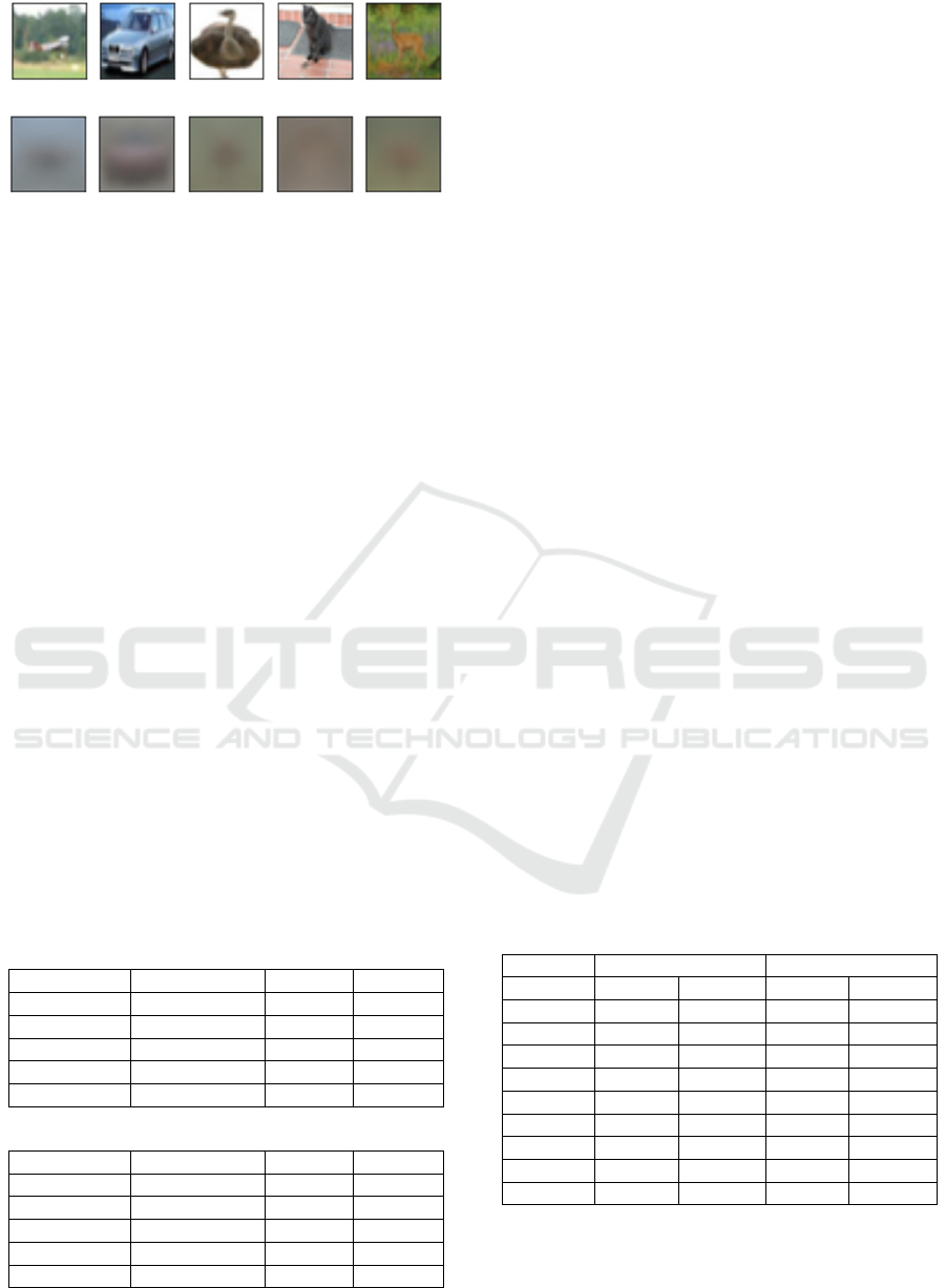
Sampled RGB images for each class

Averaged RGB images for each class

Figure 5: Examples of RGB (3-channel) image.

4 EVALUATION EXPERIMENTS

In this section we describe evaluation experiments for

validating and analysing the performance of our

proposed label representation.

4.1 Experimental Set-up

CIFAR10 and CIFAR100 (Krizhevsky, 2009) were

used for the experimental data. The training data

consists of 50,000 images (CIFAR10: 5,000 images /

class, CIFAR100: 500 images / class) and the test data

consisted of 10,000 images. Each sample was

normalized by a mean and a variance. Cropping and

horizontal flip were applied as data augmentation in

the training process. Smooth L1 loss was used as the

cost function as in (Chen, 2021). The number of

epochs was set to 300, and SGD with moment was

used as the optimizer. VGG19 (Simonyan, 2015) and

ResNet110 (He, 2016) were used as DNN models.

The architectures of the deconvolution process for

tensor representation labels are tabulated in Table 1.

Each experimental result is calculated as a median of

5 experimental results with different seed values.

Table 1: Architectures of deconvolution processes.

(a) 1 channel tensor.

ut Out

ernel Stride

64 x 1 x 1 64 x 4 x 4 4 x 4 1 x 1

64 x 4 x 4 32 x 8 x 8 4 x 4 2 x 2

32 x 8 x 8 16 x 16 x 16 4 x 4 2 x 2

16 x 16 x 16 8 x 32 x 32 4 x 4 2 x 2

8 x 32 x 32 1 x 64 x 64 4 x 4 2 x 2

(b) 3-channel tensor.

ut Out

ernel Stride

128 x 1 x 1 128 x 4 x 4 4 x 4 1 x 1

128 x 4 x 4 64 x 8 x 8 4 x 4 2 x 2

64 x 8 x 8 32 x 16 x 16 4 x 4 2 x 2

32 x 16 x 16 16 x 32 x 32 4 x 4 2 x 2

16 x 32 x 32 3 x 64 x 64 4 x 4 2 x 2

4.2 Experimental Results

4.2.1 Comparison Between Types of Labels

First, we compare the conventional one-hot vector

(Category), a speech spectrogram-based tensor label

(Speech), and a shuffled image of speech spectrum

(Shuffle) with our proposed labels consisting of

sampled grayscale images (Gray_s) and averaged

images of each class (Gray_a) from the training data.

Table 2 shows classification rates for each type of the

label representations. The subscripts (1-3) of the

labels based on the sampled and averaged images

mean as follows; The subscript of 1 means the

original image with a value range of 0 to 255. That of

2 expresses labels with -1 to 1 values by shifting and

dividing. That of 3 means the label values after the

normalization by the mean and the variance of the

training data. Table 2 shows that, when using sampled

image-based labels with normalized value ranges,

higher accuracies than the conventional spectrogram-

based labels were obtained on CIFAR10 and are

close to the accuracies given by the ordinary one-hot

vector label. These results provides that the

normalization on the value range seems to reduce

intra-class variation and emphasize diffrences

between classes. And generating a tensor with a value

range form 0 to 255 may be difficult in the

deconvolution based on the process using network

weights of 0 to 1. On the other hand, for CIFAR100,

the accuracies are conversely reduced. In particular,

when the averaged image-based labels of each class

were used, the accuracies were low under all

conditions. The reason for these results seems that the

averaged images are generally blurred as shown in

Figure 2, so this blurness maks it difficult to

distinguish between classes.

Table 2: Classification rates for each type of labels [%].

Label CIFAR10 CIFAR100

VGG ResNet VGG ResNet

Cate

93.27 94.01 72.19 72.82

eech 91.75 92.51 70.16 68.96

Shuffle 92.51 92.67 71.01 69.16

Gray_s1 91.08 92.24 66.64 66.86

Gray_s2 93.08 93.23 67.30 64.20

Gra

s3 92.91 93.12 68.16 65.96

Gra

a1 90.86 91.50 64.69 63.47

Gray_a2 91.69 90.71 59.08 50.67

Gray_a3 91.79 91.06 60.64 53.24

Next, we examine the effect of the complexity of

a tensor label. Table 3 shows results for labels applied

to sampled and averaged grayscale images with

additive noise (Noisy_Gs and Noisy_Ga) and labels

Improvement of Tensor Representation Label in Image Recognition: Evaluation on Selection, Complexity and Size

235

using noise itself (Noise_G). Table 4 shows results

using iterative addition of noise. Table 3 provides that

our tensor labels with additive noise provides higher

accuracies than one-hot vectors as well as

conventional spectrogram-based labels on the model

of VGG19. However, on the model of ResNet110, our

proposed labels were more accurate than the

spectrogram-based labels, but slightly less accurate

than the one-hot vectors. The matching between the

tensor representation and the ResNet structure is one

of subjects for future investigation. From Table 4,

more complexity derived from iterative noise

addition provides higher accuracies, but that was not

as much of an improvement as expected. And results

from both of Table 3 and 4 show that noise itself with

no class images can achieve good performances.

Table 3: Classification rates for labels with additive noise

and noise itself [%].

Label CIFAR10 CIFAR100

VGG ResNet VGG ResNet

Nois

Gs1 91.48 92.17 68.27 67.32

Noisy_Gs2 93.33 93.71 69.64 66.98

Noisy_Gs3 93.27 93.49 70.05 67.73

Nois

Ga1 91.98 92.36 68.71 67.26

Nois

Ga2 93.73 93.75 71.62 67.54

Nois

Ga3 93.67 93.70 71.52 67.78

Noise_G1 91.95 92.47 69.02 57.30

Noise_G2 93.65 93.60 71.85 67.08

Noise_G3 93.08 93.30 71.36 65.10

Table 4: Classification rates for iterative noise-added label

and iterative noise itself [%].

Label CIFAR10 CIFAR100

VGG ResNet VGG ResNet

Nois

Gs1 91.57 92.26 69.00 65.17

Nois

Gs2 93.70 93.79 71.67 69.11

Noisy2_Gs3 93.43 93.43 71.77 68.91

Noisy2_Ga1 91.45 92.25 69.43 61.62

Noisy2_Ga2 93.63 93.82 71.72 68.14

Nois

Ga3 93.57 93.75 71.86 68.01

Noise2

G1 91.27 92.26 69.63 69.93

Noise2

G2 93.68 93.73 71.76 68.00

Noise2_G3 92.61 92.76 71.45 64.31

Table 5 shows classification rates for encrypted

image-based tensors. (Crypt_Gs) means sampled

image after applying block cipher and (Crypt_Ga)

means averaged encrypted one. Table 5 shows that

more increase of complexity gives more accuracies as

in the case of labels based on images with additive

noise. Also averaged image-based label can obtain

similar accuracies to sampled image-based one. This

tendency is also similar to the case of additive noise.

Table 5: Classification rates for encrypted image [%].

Label CIFAR10 CIFAR100

VGG ResNet VGG ResNet

Gs1 91.61 92.31 69.41 60.67

Crypt

Gs2 93.86 93.79 71.92 67.83

Crypt

Gs3 93.50 93.66 71.91 67.52

Crypt

Ga1 91.52 92.45 69.71 60.90

Ga2 93.57 93.76 71.68 67.21

Ga3 93.71 93.74 71.99 67.46

We also examine the effect of increasing the

tensor sizes and the number of channels. Table 6

shows the results of the channel enhancement, that is

a 3 channelled RGB image-based tensor while

keeping the image resolution (RGB64), and the

results of enlarging image size while keeping single

channel (Gray112). Both of them means tripling the

tensor size of original tensor labels. Comparison with

Table 2 shows that a little improvement on accuracy

was obtained by increasing the number of channels to

three (RGB64) for the same image size but this is not

to the extent expected from tripling the tensor size.

And there was also no effect when the image size

(resolution) was increased keeping a single channel.

The reason for these results is assumed that the

training data is 32 pixels square and this limits the

effect of increasing the tensor size. To validate the

effectiveness of increasing tensor size, further

evaluation using larger resolution images is needed.

Table 6: Accuracies for each enhanced tensor size [%].

Label CIFAR10 CIFAR100

VGG ResNet VGG ResNet

RGB64_s1 91.07 92.58 67.81 68.29

RGB64_s2 93.24 93.14 68.34 66.11

RGB64

s3 93.00 93.24 69.04 67.43

G112

s1 90.47 92.34 65.54 67.07

G112

s2 93.06 93.42 67.32 64.94

G112_s3 92.78 93.06 68.43 65.75

Finally, we evaluated the effectiveness of the

combination between the increase of tensor size and

the complexity. Table 7 shows classification rates of

RGB-based tensor label with additive noise or after

applying block cipher. (Rs) means a label based on a

sampled RGB image. From Table 7, our proposed

label clearly outperforms conventional tensor labels

and obtained almost same accuracies as the

conventional one-hot vector representation. On the

other hand, results using Resnet110 on CIFAR100 are,

unfortunately, lower than those obtained by the one-

hot vector on the same condition. As mentioned

above, the investigation of this tendency is one of

future works.

ICPRAM 2024 - 13th International Conference on Pattern Recognition Applications and Methods

236

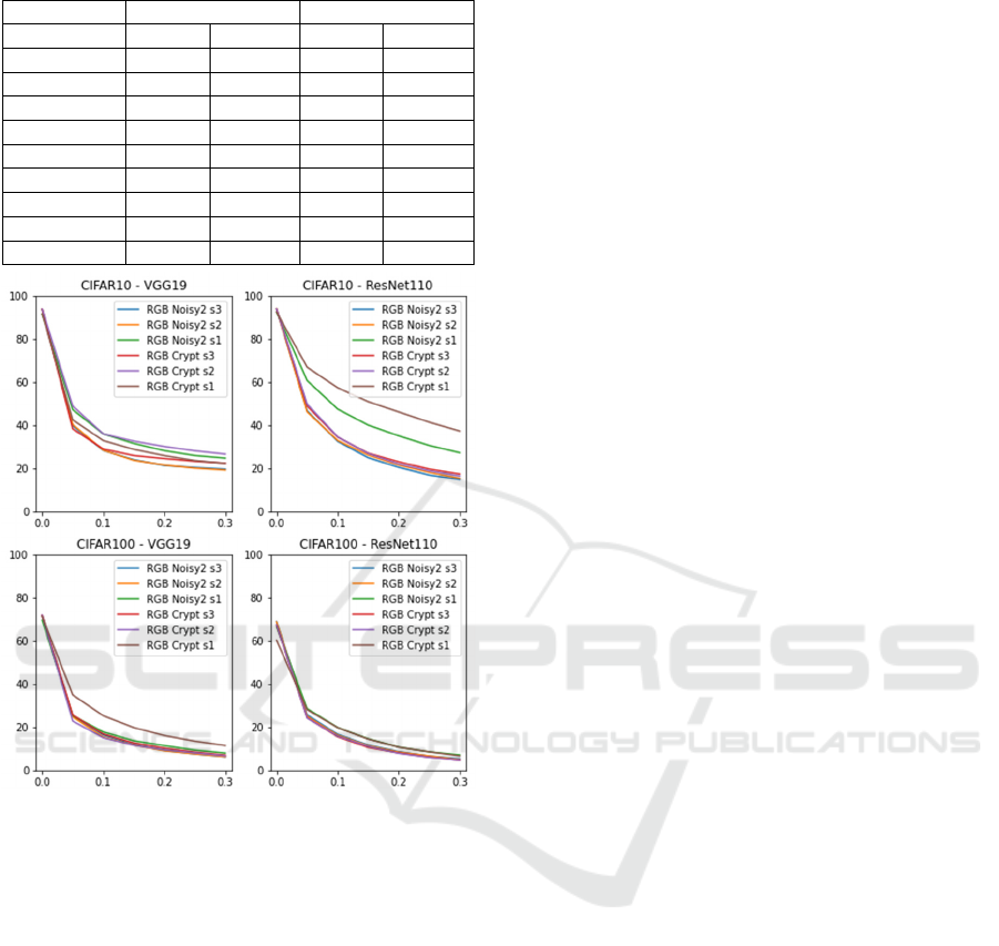
Table 7: Rates for noisy or encrypted RGB-based label [%].

Label CIFAR10 CIFAR100

VGG ResNet VGG ResNet

Nois

Rs1 91.45 92.39 69.54 66.46

Noisy2_Rs2 93.69 93.89 71.41 68.78

Noisy2_Rs3 93.58 93.80 71.37 68.86

Noise2_Rs1 91.18 92.12 70.82 61.43

Noise2

Rs2 93.63 93.94 72.20 67.76

Noise2

Rs3 93.45 93.77 72.09 66.86

Rs1 91.53 92.43 71.23 60.21

Crypt_Rs2 93.73 93.86 71.80 67.37

Crypt_Rs3 93.65 93.83 71.85 67.22

Figure 6: Accuracies on with/without normalization against

the iterative method of AEs.

4.2.2 Robustness Against AEs

We evaluated the robustness of each label against

AEs generated by the method of FGSM (Goodfellow,

2015) and the Iterative method (Kurakin, 2017). And

we adopted cases with and without a mis-recognition

target class to each algorithm. First, to investigate

how the normalization on value ranges affects the

recognition of AEs, we see accuracies among three

types of value ranges on iterative noise added and

encrypted tensors on several dataset and DNN models

against iterative method without mis-recognition

target. The reason to select this AEs method is the

most difficult to recognize them correctly. Figure 6

shows accuracies mentioned above. The horizontal

axis of each graph represents the noise level at the

time of AEs creation. Please note that all the proposed

tensors are based on sampled images. Results shown

in Figure 6 show that accuracies of each tensor vary

with conditions. From these results, we deeply

validate tensors with an original value range (0 – 255:

s1) and a value range of (-1 – 1: s2) by normalization.

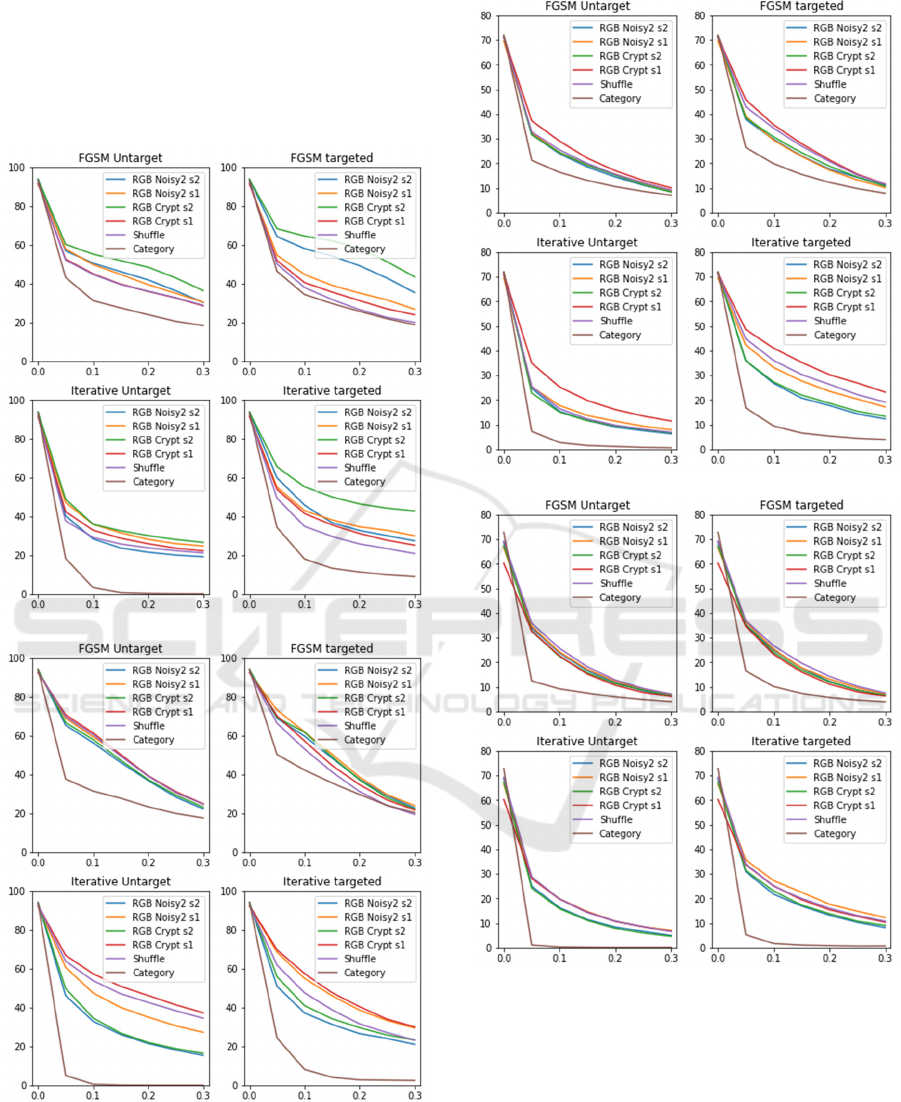
Next, we compare our proposed labels selected

above and existing labels using several datasets and

DNN models. Classification accuracies of each label

expression against AEs on CIFAR10 and CIFR100

are shown in Figure 7 and 8, respectively. Here we

use only the shuffled spectrogram-based label as the

conventional method because that are generally

superior to the basic spectrogram-based label. From

Figure 7 & 8, as evaluated in (Chen 2021), tensor

representations are more tolerant to AEs than the one-

hot vector representation, especially in the cases with

mis-recognition target. Compared to spectrogram-

based tensor representation, our proposed tensor label

often achieved higher accuracies. In particular,

among our proposed labels, post-cryptographic tensor

labels with high complexity, which were highly

accurate in 4.2.1, show higher tolerance in the cases

with mis-recognition target class. This seems to be

caused by high complexity and normalization pre-

process. On the other hand, our method did not differ

much from the conventional tensor representation

under the condition of the use of ResNet110 for

CIFAR100 similar to results in 4.2.1.

4.2.3 Impact of Number of Training Data

Finally, we validate the influence of sample number

in the training. Therefore, we examined classification

rates when the number of training data is reduced

from 20% to 1% of the standard 50,000 training data

on CIFAR10. Figure 9 shows accuracies among three

types of value ranges on iterative noise added and

encrypted tensors when using VGG19 and

ResNet110 as DNN models for validating the effect

of the normalization on value ranges. The horizontal

axis of each graph represents the percentage [%] of

the total training data actually used for training.

Please note that all of the proposed tensors are based

on sampled images. These results give that the

normalization pre-process does not always achieve

high accuracies. One of causes that tensors with

original value range of (0-255) obtained higher

accuracies seems that a wider value range can

enhance a more gap between different classes when

using limited training samples. On the other hand,

normalization process seems to narrow the

differences between classes, because a variety of

values of each dimension is smaller than that of an

ordinary tensor. Figure 10 shows the comparison

among our proposed label selected based on results in

Figure 9 and conventional labels. Figure 10 provides

Improvement of Tensor Representation Label in Image Recognition: Evaluation on Selection, Complexity and Size

237

that our tensor representations are better than the

existing tensor representation especially for less

training samples used on VGG19. when the number

of samples is large, each tensor representation label

has a similar performance but higher accuracies than

the conventional one-hot vector label.

(a) VGG19

(b) ResNet110

Figure 7: Classification rates for AEs on CIFAR10.

(a) VGG19

(b) ResNet110

Figure 8: Classification rates for AEs on CIFAR100.

ICPRAM 2024 - 13th International Conference on Pattern Recognition Applications and Methods

238

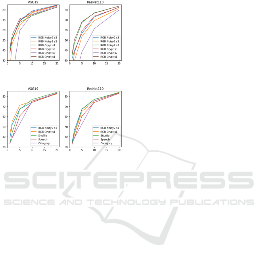
Figure 9: Classification rates among several value ranges of

tensors for each amount [%] of training data of CIFAR10.

Figure 10: Classification rates of several types of labels for

each amount [%] of training data of CIFAR10.

5 CONCLUSIONS

In this paper, we improved and evaluated the tensor

representation label proposed in (Chen, 2021) as a

different label representation in image recognition.

Specifically, improvements and evaluations were

conducted on image selection of a reference,

complexity increase, and tensor size setting. For the

reference image of the tensor representation, we

proposed sampling directly from the training data and

averaging procedures for each class. To increase

complexity, we proposed the addition of Gaussian

noise and the application of block encryption. We

also evaluated the expansion of the tensor size and the

number of channels. We also examined the varieties

of value range. In the recognition experiments

conducted for evaluating the proposed methods, our

proposed tensor representations with higher

complexity and larger sizes were as accurate as the

conventional one-hot vector for ordinary data and

more accurate than the conventional tensor

representation labels based on speech spectrograms.

In addition, in the evaluation of resistance to AEs and

experiments with reduced training data, we confirmed

that our proposed labels provide higher accuracy than

conventional labels, including one-hot vectors in

many cases. However, we unfortunately found that no

method was superior in all the cases, and that some

methods are not suitable for certain models and

datasets.

Future works include verification of the

compatibility between label types and the structure of

DNN models, and evaluation using other databases

and DNN models.

REFERENCES

Krizhevsky, A., Sutskever, I. Hinton, G. (2012). Imagenet

classification with deep convolutional neural networks.

In NIPS’12, 26th Conference on Neural Information

Processing Systems.

Szegedy, C., Vanhoucke, V., Ioffe, S., Shlens, J., Wojna, Z.

(2016). Rethinking the inception architecture for

computer vision. In CVPR’16, The IEEE/CVF

Conference on Computer Vision and Pattern

Recognition.

Hinton, G., Vinyals, O. Dean, J. (2015). Distilling the

knowledge in a neural network. In NIPS’12, 29th

Conference on Neural Information Processing Systems

Workshop.

Chen, B., Li, Y., Raghupathi, S., Lipson, H. (2021). Beyond

categorical label representations for image

classification. In ICLR’21, 9th International

Conference on Learning Representation.

Szegedy C., Zaremba, W., Sutskever, I., Bruna, J., Erhan,

D., Goodfellow, I., Fergus, R. (2014). Intriguing

properties of neural networks. In ICLR’14, 2th

International Conference on Learning Representation.

Lukasik, M., Bhojanapalli, S., Menon, A., Kumar, S.

(2020). Does label smoothing mitigate label noise? In

ICML’20, 37th International Conference on Machine

Learning.

Krizhevsky, A. (2009). Learning multiple layers of features

from tiny images.

Ehrsam, W., Meyer, C., Smith, J., Tuchman, W. (1976).

Message verification and transmission error detection

by block chaining. US Patent 4074066.

Simonyan, K., Zisserman, A. (2015). Very deep

convolutional networks for large-scale image

recognition. In ICLR’15, 3th International Conference

on Learning Representation.

He, K., Zhang, X., Ren, S., Sun, J. (2016). Deep residual

learning for image recognition. In CVPR’16, The

IEEE/CVF Conference on Computer Vision and

Pattern Recognition.

Goodfellow, I., Shlens, J., Szededy, C. (2015). Explaining

and harnessing adversarial examples. In ICLR’15, 3th

International Conference on Learning Representation.

Kurakin, A., Goodfellow, I., Bengio, S. (2017). Adversarial

examples in the physical world. In ICLR’15,

International Conference on Learning Representation

Workshop.

Improvement of Tensor Representation Label in Image Recognition: Evaluation on Selection, Complexity and Size

239