Parameter Estimation of Macroeconomic Agent-Based Models Using

Evolutionary Computation

Takahiro Obata and Setsuya Kurahashi

Graduate School of Business Sciences, Humanities and Social Sciences, University of Tsukuba, Tokyo 112-0012, Japan

Keywords:

Macroeconomic Agent-Based Models, Parameter Estimation, Evolutionary Computations, Real-Coded

Genetic Algorithms.

Abstract:

This study reports the estimation of model parameters for a macroeconomic agent-based model (ABM) using

evolutionary computation methods. In an ABM, the parameter settings of the model are important in terms

of verifying the validity of its outputs, because the parameter settings are closely related to these outputs, and

determining whether the set parameters are appropriate. Conventionally, model parameters are qualitatively

set by researchers based on values conﬁrmed from empirical studies in related ﬁelds. However, in recent years,

attempts to quantitatively determine model parameters using metaheuristic methods and Bayesian estimation-

based methods have become widespread. In this study, we attempted to estimate time-varying parameters using

a real-coded genetic algorithm, a type of evolutionary computation method, based on an inverse simulation

method, which has not been used in macroeconomic ABM parameter estimation. The analysis conﬁrmed that

parameter estimation works well when the economic conditions to be assimilated are simple, whereas it is

difﬁcult when economic conditions change in a short time, such as before and after economic shocks.

1 INTRODUCTION

This study reports the estimation of model parameters

for a macroeconomic agent-based model (MABM)

using evolutionary computation methods. When de-

veloping an agent-based model (ABM), one of the

most important issues for researchers is whether the

parameters of the model are appropriate. In addition

to the appropriateness of the parameters, parameter

settings are important in terms of verifying the va-

lidity of the outputs of the developed ABM, because

parameter settings are closely related to the outputs

of the ABM (Fagiolo, 2018). Although researchers

generally set model parameters qualitatively by re-

ferring to values conﬁrmed in empirical studies in

related ﬁelds, attempts to quantitatively determine

model parameters using metaheuristic methods or

Bayesian estimation have become widespread in re-

cent years (Delli Gatti, 2020). In this study, based

on the inverse simulation method proposed by (Ku-

rahashi, 1999) as a parameter estimation method, we

attempted to estimate the time-varying parameters of

an economic simulator using a real-coded genetic al-

gorithm (RCGA), a type of evolutionary computa-

tion method that has never been used for ABM pa-

rameter estimation in the macroeconomic ﬁeld to our

knowledge. According to the analysis results, we

conﬁrmed that parameter estimation works well when

the economic conditions to be assimilated are simple,

whereas it is difﬁcult to estimate parameters when the

economic conditions change in a short time, such as

before and after economic shocks.

2 RELATED STUDIES

2.1 MABM

As a germ of research using ABMs in macroeconomic

analysis, some of the early studies were conducted

around 1960; however, it was not until the mid-2000s

that the use of ABMs became widespread. In partic-

ular, when the ﬁnancial crisis occurred in 2008, there

was a movement to review economic analysis meth-

ods, partly because the crisis could not be predicted

using conventional analysis methods. Thus, the ef-

fectiveness of ABMs was recognized, and their use

expanded (Fagiolo, 2012).

While various models have been developed and

proposed in macroeconomic analysis utilizing ABMs,

a research paper that organized MABMs developed

since the 2000s (Dawid, 2018) identiﬁed seven major

Obata, T. and Kurahashi, S.

Parameter Estimation of Macroeconomic Agent-Based Models Using Evolutionary Computation.

DOI: 10.5220/0012313300003636

Paper published under CC license (CC BY-NC-ND 4.0)

In Proceedings of the 16th International Conference on Agents and Artiﬁcial Intelligence (ICAART 2024) - Volume 1, pages 205-212

ISBN: 978-989-758-680-4; ISSN: 2184-433X

205

MABMs/frameworks and summarized the character-

istics of each. One of these seven frameworks, com-

plex adaptive trivial systems (CATS), is frequently

used in studies focusing on emergent aspects of the

macroeconomy. (Caiani, 2016) proposed a bench-

mark model as a basis for various analyses of the

CATS framework. (Obata, 2023) listed a macroeco-

nomic approach, a sector-speciﬁc approach, and an

input–output approach as approaches for developing

an ABM to analyze the propagation of the impact

of economic shocks and developed a novel MABM

based on the benchmark model in (Caiani, 2016), uti-

lizing the strengths of each approach. In this study,

analysis is performed using a model that is an im-

proved version of the MABM developed in (Obata,

2023). The model details are presented later.

2.2 Parameterization of ABM and

Inverse Simulation Method

The setting of model parameters for ABMs is one of

the most important issues that researchers pay atten-

tion to when developing ABMs. In MABM research,

the validation of model parameters is typically con-

ducted by empirically conﬁrming whether the output

and state of the model reproduce the stylized fact.

In recent years, attempts to estimate parameters us-

ing quantitative methods have increased, but no estab-

lished quantitative parameter estimation method ex-

ists (Delli Gatti, 2020). Quantitative model param-

eter estimation methods include metaheuristic meth-

ods and methods based on Bayesian estimation such

as particle ﬁlters ((Grazzini, 2017), (Lux, 2022)).

Although attempts to estimate model parameters

quantitatively are new to the ﬁeld of MABM, vari-

ous methods have been used in ABM research as a

whole for more than 20 years. The inverse simulation

method proposed by (Kurahashi, 1999), (Kurahashi,

2013) is a pioneering study that attempted quantita-

tive parameter estimation. A typical simulation in-

volves developing a model with several parameters,

setting the parameters, running the simulation, and

adjusting the parameters based on the simulation re-

sults. Conversely, the inverse simulation method in-

volves the following process to solve a large-scale in-

verse problem:

1. designing a model with many parameters that rep-

resents the real world

2. setting up the evaluation function

3. simulation using evaluation function as objective

function

4. evaluation of the obtained initial parameters

Inverse simulation employs evolutionary computation

methods represented by genetic algorithms (GAs) as

parameter search methods. According to (Kurahashi,

2013), there are two approaches to the inverse simu-

lation method: one is to use it as inductive inference,

and the other is to use it as deductive inference. This

study attempts to estimate the parameters of MABMs

using an inverse simulation method while adopting

the former inductive reasoning approach.

2.3 Evolutionary Computations and

RCGA

Evolutionary computations are multipoint search

methods wherein the computational algorithm is in-

spired by the evolution of organisms and swarm be-

havior to perform solution search. The common

features are as follows: the population of search

points are processed in parallel and the population is

changed, there is some kind of interaction among the

search points, stochastic actions are used to change

the population, and competitive actions work among

the search points, such as survival of the ﬁttest.

A GA is a type of evolutionary computation that

incorporates the concept of natural selection, wherein

organisms that adapt to their environment survive and

those that fail to adapt die. It has the following char-

acteristics: (1) no assumption of differentiability of

the objective function is required, and (2) a global

search is possible. Although bit coding of 0 and 1 has

long been used as the genotype in GAs, when solv-

ing optimization problems with real-valued parame-

ters, the phase structure of the genotype space may

signiﬁcantly differ from that of the phenotype space,

the real number space. Therefore, a child generated

from two-parent individuals close to each other in the

phenotype space may not necessarily be generated in

the neighborhood of its parent in the phenotype space,

even if it is in the neighborhood of its parent in the

genotype space.

An RCGA, which treats real-coded vectors as

genotypes, responds to these remarks (Wright, 1991).

Because an RCGA directly manipulates real-coded

vectors by crossover, it can generate sub-populations

in the neighborhood of the parent population in the

phenotype space. Therefore, compared with conven-

tional binary coding, the solution search efﬁciency for

real-coded problems is signiﬁcantly improved. There

are various methods for RCGAs; however, in this

study, we use the distance-weighted exponential natu-

ral evolution strategy (DX-NES)(Fukushima, 2013), a

method that incorporates the concept of natural gradi-

ents. The literature reports that DX-NES improves the

performance of solution search as well as addresses

ICAART 2024 - 16th International Conference on Agents and Artiﬁcial Intelligence

206

issues such as the bad scalability of the search area.

3 ABOUT MABM USED IN THIS

STUDY

The MABM used in this study (hereinafter referred to

as the “current model” ) is the improved version of

the MABM developed by (Obata, 2023) (hereinafter

referred to as the “reference model”), which has been

improved by introducing the concept of capital goods,

etc. . In this section, we explain the main differences

from the reference model and discuss the simulation

results using the current model.

3.1 Major Differences Between

Reference and Current Models

The concept of capital equipment, which is one of the

remaining limitations of the reference model, is intro-

duced into the current model. All ﬁrms use capital

equipment to produce their products. The produc-

tivity of capital equipment, µ

, which represents the

number of products that can be produced per piece of

capital equipment, is set at 1.5 for all ﬁrms and all

capital equipment. The labor capital equipment ratio,

, which represents the maximum number of capi-

tal equipment that a worker can be equipped with, is

6.4. These two values were set referring to (Caiani,

2016). Thus, the maximum number of products that a

worker can produce in one step is 1.5 ∗6.4 = 9.6. The

durability period of capital equipment, η

, was set to

20 steps (equivalent to 5 years in the real world). This

was determined by referring to the table of useful lives

of major depreciable assets published by the National

Tax Administration Agency of Japan. The ﬁrms deter-

mine the desired number of capital facilities assumed

for the current period using the following formula.

f i,t

= (1 + g

f i,t

f i,t−1

(1)

f i,t

= γ

pc f r

f i,t−1

− ¯r

¯r

+ γ

f i,t−1

− ¯u

¯u

, (2)

where K

f i,t

denotes ﬁrm i’s desired number of capital

facilities in period t, g

f i,t

denotes the desired capital

facility growth rate, and K

f i,t−1

denotes the number

of capital facilities owned in period t − 1. γ

, γ

, ¯r,

and ¯u denote constants and are set to 0.01, 0.02, 0.03,

and 0.90, respectively. These values are taken from

(Caiani, 2016). pc f r

f i,t−1

denotes the net asset cash

ﬂow multiplier for ﬁrm i in period t − 1, where the to-

tal capital equipment held is added to the calculation

of net assets, as deﬁned in the reference model. The

investment amount of capital equipment purchased in

each period is not reﬂected in the operating cash ﬂow

calculation because it is a capital transaction. There-

fore, the operating cash ﬂows in the reference and cur-

rent models are the same. The net asset cash ﬂow

multiples in the current model are as follows:

pc f r

f i,t

OCF

f i,t

f i,t−1

(3)

f i,t

= reference models’ NW

f i,t

+ KV

f i,t

,(4)

where KV

f i,t

denotes the total value of capital facili-

ties owned by ﬁrm i in period t. The capital equip-

ment owned by ﬁrm i is assumed to be depleted by

1/η ∗ ν

ηk

in each period. Firm i orders the quantity

of capital equipment it wishes to own, i.e., 1/η

∗

f i,t

∗ (1 + g

f i,t

), in each period. However, the abil-

ity to procure capital equipment based on the quan-

tity ordered depends on the availability of sufﬁcient

products for capital equipment. The mechanism for

ordering and procuring capital equipment is based on

(Poledna, 2023), where the required quantity of cap-

ital equipment is aggregated by the industry attribute

of the ﬁrms, and the products produced by each ﬁrm

are provided according to its share of product sales in

the industry to which it belongs in the immediately

preceding period, rather than directly between indi-

vidual ﬁrms with supplier–customer relationships, as

in the case of product sales. Thus, a ﬁrm provides

the products it produces in proportion to its share of

product sales in its industry in the previous period.

Although the percentage of the products of each in-

dustry comprising a unit of capital equipment can be

set differently for each industry, in the setting of the

current model, the percentage of the products of each

industry comprising a unit of capital equipment is as-

sumed to be equal. The maximum quantity of prod-

ucts that a ﬁrm can provide for capital equipment in

each period is limited to 3% of the quantity of prod-

ucts manufactured in the period. How many products

a ﬁrm can produce depends on the number of workers

and intermediate input materials it has in the reference

model; however, in the current model, it also depends

on the number of capital facilities it has.

max

f i,t

= min{mat

1, f i,t

/inpq

f i,1

,mat

2, f i,t

/inpq

f i,2

,··· ,

mat

n, f i,t

/inpq

f i,n

,µ

f i,t

,µ

f i,t

where mats,

f i,t

denotes the quantity of intermediate

input materials s in stock for ﬁrm i in period t. inpq

f i,s

denotes the quantity of intermediate input materials

required by ﬁrm i to produce a unit of product, and

f i,t

denotes the number of workers employed by

ﬁrm i in period t. Because of the introduction of

the capital equipment concept in the current model,

the method of updating product markups has changed

from that in the reference model. The product markup

Parameter Estimation of Macroeconomic Agent-Based Models Using Evolutionary Computation

207

is the percentage that ﬁrm i adds to the product man-

ufacturing cost uc when setting the product price p

in step t, and their relations can be expressed as

f i,t

= uc

f i,t

∗(1+mu

f i,t

). In the reference model, the

only criterion for increasing or decreasing the prod-

uct markup is whether the product inventory ratio ex-

ceeds the threshold value ν. However, in the current

model, we introduced a capital equipment utilization

criterion, u

threshold

, and added another condition indi-

cating whether u

threshold

is more than 95%. This is

done to avoid raising the product markup when the

product inventory ratio becomes low under the con-

dition of low facility utilization. The current model

differs from the reference model in many other ways

because of the introduction of the capital equipment

concept (e.g., the capital equipment sales volume is

reﬂected in the calculation of expected product sales

volume). However, these are minor changes and will

not be explained here.

3.2 Simulation Results

This section reports the simulation results with the

model parameters based on the reference model.

Figure 1: Mean and standard deviation of each indicator

value obtained from ten trials of simulation up to 150 steps.

Figure 1 plots the mean value and ±1 standard de-

viation of the results of each trial, excluding the two

trials wherein the economy collapsed, after running

the 150-step simulation ten times. The price index

is calculated by taking the weighted average of the

average prices of ﬁrm and household products. Ac-

cording to the transition in nominal GDP, the standard

deviation is within a small range in the early stage

of the simulation; subsequently, the standard devia-

tion gradually increases. This movement is similar

to that of the reference model. As a common trend

observed in the other index values, the standard de-

viations are within a small range in the ﬁrst 10–20

steps of the simulation. In the subsequent steps, the

standard deviations of the price index, unemployment

rate, and the number of corporate bankruptcies grad-

ually increase, whereas the standard deviations of the

real GDP growth rate and the rate of change in the

price index exhibit a slight tendency to increase until

steps 60-80; however, thereafter, they remain within

a narrow range. In the early stages of the simulation,

the results of each simulation are similar to those of

the reference model even though the degree of move-

ment is signiﬁcant, partly due to the initial settings.

According to the standard deviation of the real GDP

growth rate and the price index change rate, the sim-

ulation results were mixed until approximately the

80th step, after which each simulation reached a sim-

ilar economic state. Excluding the initial stage by

the 35th step, where output ﬂuctuations were signif-

icant, the average values per step (standard deviation

in parentheses) were as follows: nominal GDP growth

rate was approximately 0.73% (0.68%), price inﬂa-

tion rate was 0.47% (0.14%), real GDP growth rate

was approximately 0.26% (0.68%), and GDP growth

rate was approximately 0.26% (0.68%). (0.68%) and

an unemployment rate of 23% (0.63%). These lev-

els are close to the reference model’s nominal GDP

growth rate of approximately 0.86% (0.9%), price in-

ﬂation rate of 0.43% (0.08%), real GDP growth rate

of approximately 0.44% (0.9%), and unemployment

rate of 19% (3.3%).

4 PARAMETER ESTIMATION

METHOD BY EVOLUTIONARY

COMPUTATION

Based on the MABM simulation results discussed in

the previous section, it takes approximately 80 steps

for the model behavior to converge to similar behav-

ior in each simulation. Therefore, when estimating

model parameters in evolutionary computation, the

results of simulation runs of up to 100 steps are used

as initial conditions with some buffer, and the model

parameters estimated using evolutionary computation

are reﬂected in the computation process of the simu-

lation after the 100th step.

As the parameter estimation method, DX-NES

is adopted, which is an evolutionary computation

method that has high solution search performance and

can achieve the optimal solution with fewer individual

evaluations. The parameters of DX-NES are set ac-

ICAART 2024 - 16th International Conference on Agents and Artiﬁcial Intelligence

208

cording to the reccomendation of (Fukushima, 2013),

except for the number of individuals explained later.

In the MABM parameter estimation in this study,

the evaluation values of the RCGA individuals depend

on the results of the MABM simulations. Therefore,

it is necessary to run MABM simulations to obtain in-

dividual evaluation values, which is computationally

expensive. DX-NES is suitable for the case in this

study. According to (Fukushima, 2013), because DX-

NES allows parallel execution of the solution evalu-

ation value calculation, the calculation time per gen-

eration does not signiﬁcantly change even when the

number of individuals to be generated is increased to

the extent that parallel computing resources permit.

In this case, as the number of individuals generated

increases, the number of generations required to ﬁnd

the optimal solution generally decreases. Consider-

ing the available machine speciﬁcations, the number

of individuals to be generated and evaluated per gen-

eration is set to 28.

The value of each individual is evaluated on the

basis of the absolute error between the time series of

each social indicator value to be assimilated and the

time series of social indicator values obtained from

the output of MABMs. The absolute error rather than

the squared error is used because we do not want

to focus on outliers in the output of the time series

but rather on the overall direction of the social in-

dicator values to be assimilated. The ﬁrst step in

the process of calculating speciﬁc evaluation values

is to select the social indicators to be assimilated. In

this study, three indicators were selected: real GDP

growth rate, nominal GDP growth rate, and price in-

dex growth rate. Next, the MABM simulation is run

for 101-124 steps, using the set of MABM parame-

ters represented by the genes of each individual in the

evolutionary computation, and the social index values

are calculated on the basis of the output. The reason

why 24 MABM simulation steps are performed is that

the economic situation in an MABM artiﬁcial soci-

ety does not change immediately after each step, and

there is a lag until the impact of the parameters gen-

erated by evolutionary computation is reﬂected in the

economic situation. Even after the economic situation

is reﬂected, we cannot conﬁrm whether the economic

situation is stable until a certain length of time has

passed. Finally, the absolute error between the social

indicator value to be assimilated and the social indi-

cator value obtained from the MABM is calculated,

and the sum of the absolute errors of the three social

indicator values is used as the individual’s evaluation

value. However, if the value of the gene of each indi-

vidual deviated from the initially set upper and lower

limits, the MABM simulation was not performed, the

absolute value of the value exceeding the upper and

lower limits was calculated for all genes possessed by

each individual, and the sum of these values multi-

plied by 100,000 was used as the evaluation value for

each individual as a penalty.

5 VALIDATION OF PARAMETER

ESTIMATION RESULTS

Because the MABM used in this study has many pa-

rameters, optimization using evolutionary computa-

tion is performed for parameters that affect agent be-

havior, excluding the setting parameters, such as the

number of agents, and parameters with external vari-

ables in the economic environment, such as policy in-

terest rates and tax rates.

5.1 Parameter Estimation Results

Table 1 shows the parameters estimated for parame-

ter optimization. For these parameters, the analysis

was performed in two patterns, one assuming stable

economic growth and the other assuming economic

downturn.

In the case of stable economic growth, the pa-

rameters were optimized using evolutionary compu-

tation ﬁve times using time-series data with 24 con-

secutive steps of 0.80% nominal GDP growth, 0.40%

price index increase, and 0.40% real GDP growth as

the transition of social indices to be assimilated to

these parameters. Conversely, in the case of an eco-

nomic downturn, the parameters were optimized us-

ing evolutionary computation ﬁve times using time-

series data with 24 consecutive steps of -0.40% nomi-

nal GDP growth rate, -0.20% price index growth rate,

and -0.20% real GDP growth rate as the social indica-

tors to be assimilated.

Table 2 shows the mean of the estimated values

of all individuals in the last generation of each trial

for both stable economic growth and downturns. Two

parameters for the capital equipment rate, u

threshold

and ¯u, were estimated to have lower values for sta-

ble growth. Because one condition for raising the

markup is for the capital equipment utilization rate

to be above u

threshold

, a lower u

threshold

is more likely

to promote a higher markup, leading to the conclu-

sion that prices are more likely to raise in the stable

growth case. ¯u denotes the threshold for increasing

the facility growth rate, and the lower the ¯u, the more

likely that the facility growth rate will increase. Be-

cause increasing the number of facilities and the quan-

tity of products produced leads to economic growth,

it is natural that the estimated value of ¯u is smaller

Parameter Estimation of Macroeconomic Agent-Based Models Using Evolutionary Computation

209

Table 1: List of model parameters to be estimated.

ν estimated inventory to product

sales volume ratio

0.10 1.00 0.00

λ weight of previous period’s val-

ues in the current period forecast

0.25 1.00 0.00

threshold

One of the thresholds at which

the markup is raised. Raise the

markup if capital equipment uti-

lization is above this threshold

and other conditions are also met

0.95 1.00 0.50

¯r One of the factors that determine

the capital equipment growth

rate. If the proﬁt margin is above

this value, the capital equipment

growth rate may be increased.

0.03 0.20 0.00

¯u One of the factors that determine

the capital equipment growth

rate. If the capital equipment uti-

lization rate is above this value,

the capital equipment growth

rate can be increased.

0.90 1.00 0.50

γ1 One of the factors that determine

the capital equipment growth

rate. Adjustment terms for proﬁt

margins.

0.01 0.10 0.00

γ2 One of the factors that determine

the capital equipment growth

rate. Adjustment term for capi-

tal equipment utilization.

0.02 0.10 0.00

ratio

w f c

Adjustment rate coefﬁcient for

the number of workers.

0.50 1.00 0.00

One of the factors that determine

household consumption expen-

diture. Coefﬁcient of household

income.

0.40 1.00 0.00

One of the factors that determine

household consumption expen-

diture. Coefﬁcient of household

assets.

0.25 1.00 0.00

for stable growth. adaptiveλ denotes a parameter that

affects each agent’s calculation of expectations, con-

trolling the weight between the actual and expected

values one period ago. The larger the adaptiveλ, the

greater the weight of the performance of the previ-

ous period. Therefore, a larger adaptiveλ may be

more likely to continue the previous period’s situa-

tion; however, whether this has a positive or negative

effect on the economy depends on the situation.

We review the evolution of economic indicators

that reﬂect the parameters estimated by evolutionary

computation in each economic situation. Figure 2

shows the evolution of each social indicator value for

stable growth. The graphs of all social indicators are

perfectly consistent up to the 100th step because the

common economic situation is read into the param-

eter estimation up to this step. The 101st step and

beyond show that nominal GDP is rising steadily and

the unemployment rate is declining. The mean value

(standard deviation) of each indicator value is as fol-

Table 2: Parameter estimation results.

Parameters Stable growth Downturn

ν 0.31 0.32

adaptiveλ 0.31 0.37

threshold

0.68 0.75

¯r 0.12 0.14

¯u 0.71 0.73

γ1 0.01 0.02

γ2 0.03 0.04

ratio

w f c

0.33 0.28

0.34 0.30

0.30 0.33

lows. The mean (standard deviation) of each indi-

cator value was +0.96% (+0.44%) for nominal GDP

growth, +0.82% (+0.08%) for price index growth, and

+0.14% (+0.39%) for real GDP growth. Figure 3

shows the same values for the economic downturn.

In Figure 3, the nominal GDP growth rate is ﬂat im-

mediately after the 100th step, which is different from

the case of stable economic growth. The other major

differences from the stable growth case are the large

angle of the price index and the fact that the unem-

ployment rate, on average, remains ﬂat. The nominal

GDP growth rate was +0.49% (+0.56%), the price in-

dex change rate was +0.92% (+0.14%), and the real

GDP growth rate was -0.43% (+0.52%), resulting in

lower nominal and real GDP growth rates than those

in the case of stable growth. Although the rate of price

index change exceeded the level of stable growth, be-

cause the three social index values were used to gener-

ate the individual valuation values, it may have been

easier to increase the individual valuation values by

reducing the errors in the two GDP growth rates, even

if the error in the rate of price index change increased.

This is an example of how evolutionary computation

may search for extreme solutions when there are mul-

tiple social indicators to be assimilated during param-

eter optimization. How to set the values of the social

indicators to be assimilated is for future studies.

Figure 2: Mean and standard deviation of transition of each

indicator value in stable growth case.

ICAART 2024 - 16th International Conference on Agents and Artiﬁcial Intelligence

210

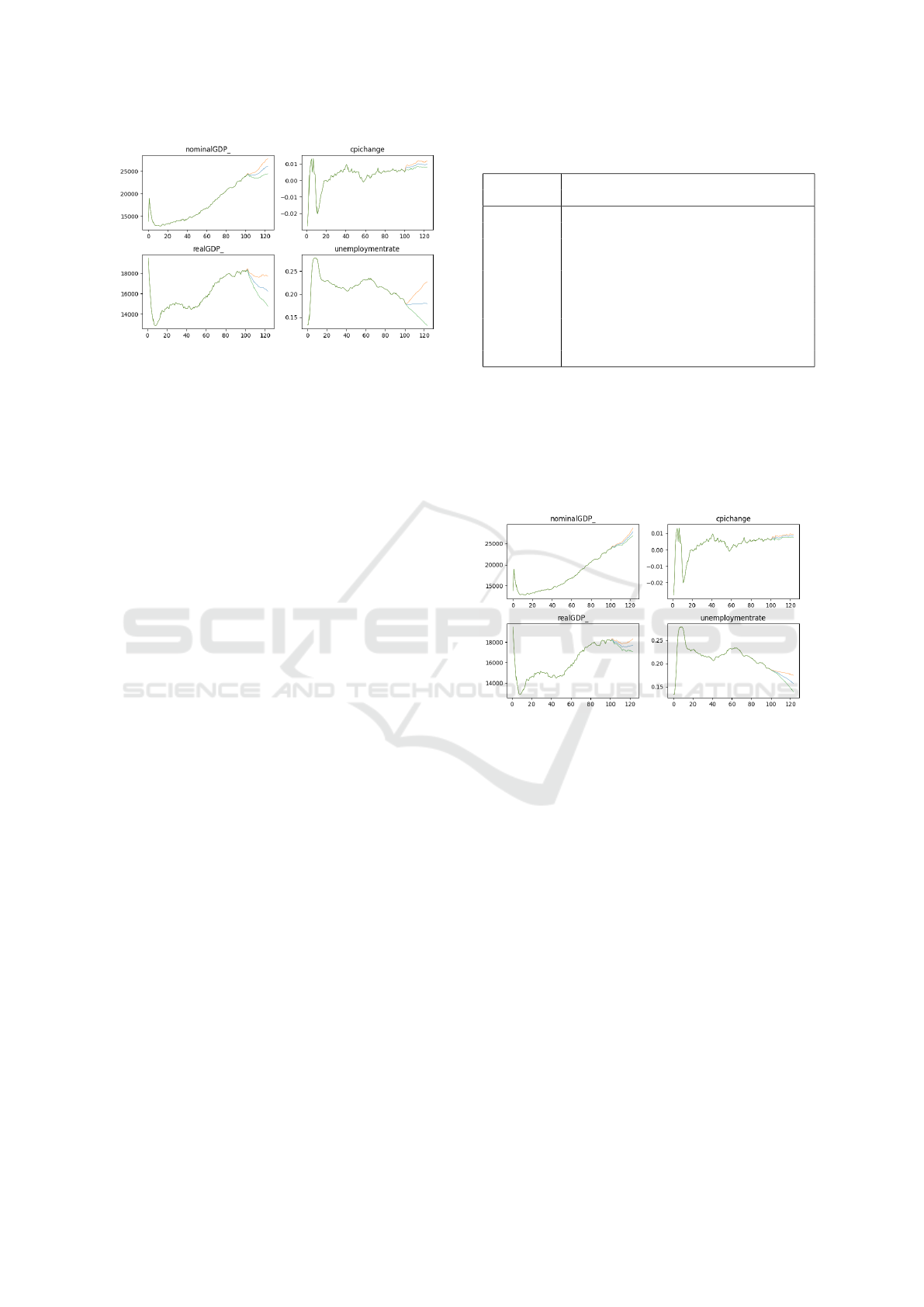
Figure 3: Mean and standard deviation of transition of each

indicator value in downturn case.

5.2 Parameter Estimation in Cases

Where Economy Moves up and

down in the Short Term

Next, we tested whether appropriate parameter es-

timation can be performed even when the economy

moves up and down in the short term. When an eco-

nomic shock occurs, the economic situation changes

both before and after the shock. Therefore, it is nec-

essary to check whether the model parameters change

because of changes in the economic situation. There-

fore, assuming that there are ups and downs in the

economy, we prepared time-series data for a period

of stable growth before the economic shock, a pe-

riod of rapid economic decline, and a period of re-

covery after the shock was resolved; we conducted

parameter optimization. The initial eight steps of the

time-series data assumed stable growth, with nominal

GDP growth of 0.80%, price index growth of 0.40%,

and real GDP growth of 0.40%, followed by a shock

period for eight steps with nominal GDP growth of -

0.60%, price index growth of -0.20%, and real GDP

growth of -0.40%. Thereafter, the shock resolution

period for four steps is assumed during which the

nominal GDP growth rate, price index inﬂation rate,

and real GDP growth rate hover at 0.00%. Eventu-

ally, the economy returns to a period of stable growth

in four steps. We also performed parameter estima-

tion for ten parameters in the case of business ﬂuctu-

ations. Table3 presents the results of parameter opti-

mization for the business ﬂuctuation case. For ref-

erence, the results for stable growth and economic

downturn from the previous section are also included.

Table3 shows that many parameters are between the

two cases of stable growth and economic downturn,

or close to them.

After the 101st step in the case of business ﬂuc-

tuations, the nominal GDP growth rate was +0.64%

(+0.51%), the price index growth rate was +0.79%

Table 3: Parameter search results for ﬂuctuation case.

Parameters

business (Reiterated) (Reiterated)

ﬂuctuation Stable growth Downturn

ν 0.22 0.31 0.32

adaptiveλ 0.38 0.31 0.37

threshold

0.69 0.68 0.75

¯r 0.12 0.12 0.14

¯u 0.72 0.71 0.73

γ1 0.02 0.01 0.02

γ2 0.05 0.03 0.04

ratio

w f c

0.43 0.33 0.28

0.44 0.34 0.30

0.29 0.30 0.33

(+0.07%), and the real GDP growth rate was -0.13%

(+0.47%). The simulation results fall between stable

growth and economic downturn, implying that the es-

timation results capture the business ﬂuctuation situ-

ation to some extent. Figure 4 shows the evolution of

each indicator simulated using the estimated parame-

ters for the business ﬂuctuation case.

Figure 4: Mean and standard deviation of transition of each

indicator value in business ﬂuctuation case.

Although the average values alone do not reveal

this, according to the output of individual simulators,

for example, there are cases wherein real GDP, af-

ter leveling off, exhibits an upward trend in the sec-

ond half of the period and cases wherein it exhibits a

downward trend in the middle of the period and levels

off in the last half, indicating that some of the charac-

teristics of the business ﬂuctuation cases are captured.

However, overall, the economic transition was differ-

ent from the ups and downs in the economy. It is dif-

ﬁcult to ﬁt short-term upward and downward move-

ments when the model parameters are ﬁxed through-

out the simulation period.

6 CONCLUSION

In this study, we attempted to estimate the parame-

ters of MABMs, which is an important issue when us-

Parameter Estimation of Macroeconomic Agent-Based Models Using Evolutionary Computation

211

ing an ABM, by RCGA. Conventionally, researchers

have set the parameters of ABMs by referring to styl-

ized facts. However, in recent years, an increas-

ing number of studies have attempted to estimate

the parameters of ABMs using quantitative methods

such as heuristic methods or Bayesian estimation-

based methods. In this study, we attempted to esti-

mate time-varying model parameters using evolution-

ary computation methods based on the concept of the

inverse simulation method proposed by (Kurahashi,

1999). From the experimental results, we conﬁrmed

that parameter estimation by evolutionary computa-

tion works well in cases where the economic transi-

tion to be assimilated is stable. On this basis, we con-

ﬁrmed that parameter search using evolutionary com-

putation works well as an inverse simulation method.

Conversely, we conﬁrmed that it is difﬁcult to esti-

mate appropriate parameters in cases where the eco-

nomic situation to be assimilated changes in the short

term. One reason for this may be that it may be difﬁ-

cult to ﬁt the economic ﬂuctuations in the short term

with ﬁxed model parameters.

One of our future tasks will be to develop a more

appropriate method of measuring the evaluation val-

ues of individuals in evolutionary computation. Cur-

rently, the absolute error is calculated for multiple so-

cial indicators to be assimilated, and the sum of these

values is used as the individual’s evaluation value.

However, it may be more appropriate to use a single

social indicator. As described in the previous section,

it is difﬁcult to evaluate parameters when multiple in-

dicators are used, some of which are good while oth-

ers are not. The second issue is to develop a method

for capturing changes in parameter values in the short

term. In the analysis of this study, the economic sim-

ulator was run for 24 steps to evaluate each individ-

ual. The parameters used in the simulation reﬂected

the parameters estimated by evolutionary computa-

tion in the economic simulator only at the beginning

of the simulation, and the reﬂected parameters were

then continued. This is because the genes of each in-

dividual in the RCGA corresponded to each MABM

parameter. We would like to conﬁrm as a future issue

whether it is possible to capture changes in parameter

values in cases wherein economic conditions change

in the short term by setting genes corresponding to

each parameter at each point in time.

REFERENCES

Fagiolo, G. and Richiardi, M. (2018). Empirical

validation of agent-based models. Agent-Based

Models in Economics: A Toolkit (pp. 163–182).

Cambridge: Cambridge University Press.

Delli Gatti, D. and Grazzini, J. (2020). Rising to the

challenge: bayesian estimation and forecasting

techniques for macroeconomic agent based mod-

els. Journal of Economic Behavior and Organi-

zation, Vol.178, pp.875–902.

Fagiolo, G. and Roventini, A. (2012). Macroeco-

nomic policy in dsge and agent-based models..

Revue de l’OFCE, Vol.124, No.5, pp.67–116.

Dawid, H. and Delli Gatti, D. Agent-based macroe-

conomics. (2018). Handbook of Computational

Economics, Vol.4, Elsevier, pp.63–156.

Caiani, A., Godin, A., Caverzasi, E., Gallegati, M.,

Kinsella, S. and Stiglitz, J. (2016). Agent based-

stock ﬂow consistent macroeconomics: Toward

a benchmark model. Journal of Economic Dy-

namics and Control, Vol.69, pp.375–408.

Obata, T., Sakazaki J., and Kurahashi, S. (2023)

Building a macroeconomic simulator with multi-

layered supplier–customer relationships. Risks,

Vol.11 ,No.7, pp. 128.

Grazzini, J., Richiardi, M. G., and Tsionas, M.

(2017). Bayesian estimation of agent-based

models. Journal of Economic Dynamics and

Control, Vol.77, pp.26–47.

Lux, T. (2022). Bayesian estimation of agent-based

models via adaptive particle markov chain monte

carlo. Computational Economics 60, pp.451–

477.

Kurahashi, S. (2013). State-of-the-art of social system

research : model estimation and inverse simu-

lation. (Japanese) Journal of the Society of In-

strument and Control Engineers Vol. 52, No. 7,

pp.588–594.

Kurahashi, S., Minami, U., and Terano, T. (1999). In-

verse Simulation for analyzing models of artiﬁ-

cial societies. (Japanese) Transactions of the So-

ciety of Instrument and Control Engineers Vol.

35, No. 11, pp.1454–1461.

Alden H. Wright. (1991). Genetic algorithms for real

parmter optimization. Foundations of Genetic

Algorithms, pp.205–218.

Fukushima, N., Nagata, Y., Kobayashi, S. and Ono,

I. (2013). Distance-weighted exponential natu-

ral evolution strategy and its performance evalu-

ation. (Japanese) Transaction of the Japanese So-

ciety for Evolutionary Computation Vol. 4, No.

2, pp.57–73.

Poledna, S., Miess, M. G., Hommes, C., and Ra-

bitsch, K. (2023). Economic forecasting with an

agent-based model. European Economic Review

Vol. 151, 104306.

ICAART 2024 - 16th International Conference on Agents and Artiﬁcial Intelligence

212