Improving Parameter Training for VQEs by Sequential Hamiltonian

Assembly

Jonas Stein

1,2

, Navid Roshani

, Maximilian Zorn

, Philipp Altmann

, Michael Kölle

and

Claudia Linnhoff-Popien

LMU Munich, Germany

Aqarios GmbH, Munich, Germany

ﬁ

Keywords:

Quantum Computing, Learning, Parameters, Iterative, VQE.

Abstract:

A central challenge in quantum machine learning is the design and training of parameterized quantum circuits

(PQCs). Similar to deep learning, vanishing gradients pose immense problems in the trainability of PQCs,

which have been shown to arise from a multitude of sources. One such cause are non-local loss functions,

that demand the measurement of a large subset of involved qubits. To facilitate the parameter training for

quantum applications using global loss functions, we propose a Sequential Hamiltonian Assembly (SHA)

approach, which iteratively approximates the loss function using local components. Aiming for a prove of

principle, we evaluate our approach using Graph Coloring problem with a Varational Quantum Eigensolver

(VQE). Simulation results show, that our approach outperforms conventional parameter training by 29.99%

and the empirical state of the art, Layerwise Learning, by 5.12% in the mean accuracy. This paves the way to-

wards locality-aware learning techniques, allowing to evade vanishing gradients for a large class of practically

relevant problems.

1 INTRODUCTION

One of the most promising approaches towards

an early quantum advantage is quantum machine

learning based on parameterized quantum circuits

(PQCs) (Cerezo et al., 2021a). PQCs are gener-

ally regarded as the quantum analog to artiﬁcial neu-

ral networks, as they resemble arbitrary function ap-

proximators with trainable parameters (Schuld et al.,

2021). Mathematically, PQCs are parameterized lin-

ear functions that live in an exponentially high di-

mensional Hilbert space with respect to the number of

qubits involved. In essence, the ability to efﬁciently

execute speciﬁc computations in this large space al-

lows for provable quantum advantage (Grover, 1996;

Deutsch and Jozsa, 1992).

A core difference in a gradient based training

process of classical ANNs with PQCs, is the efﬁ-

ciency: While the gradient calculation is invariant

in the number of parameters in classical ANNs, its

runtime complexity evidently scales linearly with the

number of parameters for PQCs (Mitarai et al., 2018).

As a gradient is merely the expectation value of the

probabilistic measurement from a quantum circuit,

its error-dependent runtime scaling is O (1/ε) com-

pared to the classical O (log(1/ε)) (Knill et al., 2007).

This disadvantage manifests substantially in case of

vanishing gradients, which are a common problem

in PQCs (McClean et al., 2018), especially as the

gradients can vanish exponentially in the number of

qubits (McClean et al., 2018), as opposed to the num-

ber of layers in the classical case (Bradley, 2010; Glo-

rot and Bengio, 2010).

Subsequently, much attention was devoted to ex-

ploring causes of vanishing gradients for PQCs by the

scientiﬁc community, which identiﬁed the four fol-

lowing possible causes of vanishing gradients:

1. Expressiveness: The larger the reachable sub-

space of the Hilbert space, the more likely gra-

dients can vanish (Holmes et al., 2022).

2. The locality of the measurement operator associ-

ated with the loss function: The more qubits have

to be measured, the more likely gradients can van-

ish (Cerezo et al., 2021b; Uvarov and Biamonte,

2021; Kashif and Al-Kuwari, 2023).

3. The entanglement in the input: The more en-

tangled or random the initial state, the more

likely gradients can vanish (McClean et al., 2018;

Cerezo et al., 2021b).

Stein, J., Roshani, N., Zorn, M., Altmann, P., Kölle, M. and Linnhoff-Popien, C.

Improving Parameter Training for VQEs by Sequential Hamiltonian Assembly.

DOI: 10.5220/0012312500003636

Paper published under CC license (CC BY-NC-ND 4.0)

In Proceedings of the 16th International Conference on Agents and Artiﬁcial Intelligence (ICAART 2024) - Volume 2, pages 99-109

ISBN: 978-989-758-680-4; ISSN: 2184-433X

4. Hardware noise: The more noise and the more

different noise types present in hardware, the

more likely measured gradients can vanish (Wang

et al., 2021; Stilck França and Garcia-Patron,

2021).

More recently, mathematical approaches unifying the

theory underlying causes were proposed, allowing for

a quantiﬁcation of the presence of vanishing gradi-

ents in a given PQC (Ragone et al., 2023; Fontana

et al., 2023). Similar to the vanishing gradients prob-

lem in classical machine learning, many techniques

are being investigated in related work (see (Ragone

et al., 2023) for an overview). Some concrete exam-

ples to this are clever parameter initialization (Zhang

et al., 2022) and adaptive, problem informed learning

rates (Sack et al., 2022).

In this article we propose another approach to fa-

cilitate efﬁcient parameter training in PQCs coined

Simulated Hamiltonian Assembly (SHA), which is

targeted towards the issue of locality. In essence, we

propose to exploit the structure of most practically

employed measurement operators

H, i.e.,

H =

∑

where

is a local Hamiltonian for all i. In this

context, locality means that the given operator only

acts non-trivially on a small subset of all qubits, such

that the loss is merely inﬂuenced by the outcome of

a small subset of qubits. An important class of prob-

lems exemplifying the property of having a local de-

composition while also being a promising contender

towards quantum advantage are combinatorial opti-

mization problems (Lucas, 2014; Albash and Lidar,

2018; Pirnay et al., 2023).

Inspired from iterative learning approaches like

layerwise learning from (quantum) machine learning

and iterative rounding from optimization, SHA starts

with a partial sum of the measurement operator

(e.g., simply

) and iteratively adds more terms un-

til it completely assembled the original measurement

operator

H. This iterative approximation of the loss

function allows to start with a local measurement op-

erator, which increases the ease of ﬁnding good initial

parameters outside potential barren plateaus (i.e., ar-

eas in which the gradient vanishes), and subsequently

aims to continually evade barren plateaus until the

complete, typically global, measurement operator is

used.

As a proof of principle, we conduct a case study

for the problem of graph coloring using the state of

the art PQCs based approaches to do so: The Varia-

tonal Quantum Eigensolver (VQE) and the Quantum

Approximate Optimization Algorithm (QAOA). The

problem of graph coloring is chosen, as it has a com-

plex loss function which challenges standard param-

eter training approaches and furthermore allows for

a comparison of different assembly approaches. Our

evaluation shows a signiﬁcant improvement in solu-

tion quality when using SHA compared to standard

gradient descent based training, as well as compara-

ble state of the art approaches from related work.

2 BACKGROUND

In this section, we present the fundamental theory be-

hind training parameters in PQCs, and also introduce

the algorithms used for evaluation.

2.1 Training Parameterized Quantum

Circuits

Similar to classical machine learning, most prac-

tically employed parameter training techniques for

PQCs rely on gradient based methods. The corner-

stone for calculating the gradients of a PQC U (θ,x),

where U is a unitary matrix acting on all n qubits,

x ∈ C

denotes the data input and θ ∈ R

the param-

eters, is the Parameter Shift Rule. Exploiting that

all PQCs can be decomposed into possibly parame-

terized single qubit gates and non-parameterized two

qubit gates (Nielsen and Chuang, 2010), the param-

eter shift rule takes advantage of the periodic nature

of single qubit gates. Similar to how

/dx sin(x) =

sin(x +

/2), one can show that ∀i:

∂

∂θ

U (θ,x)|ψ⟩ =

U (θ

,x)|ψ⟩ −U (θ

−

,x)|ψ⟩

, (1)

where |ψ⟩ denotes an arbitrary initial state and

= (θ

,...,θ

i−1

,θ

/2, θ

i+1

,...,θ

) (Mitarai

et al., 2018; Schuld et al., 2019). This allows utilizing

the original PQC U to calculate the gradient as

efﬁciently as the forward pass for each parameter,

which can be parallelized using multiple QPUs to

achieve the same runtime complexity as the backward

pass in classical ANNs, when neglecting error.

2.2 The Variational Quantum

Eigensolver

The Variational Quantum Eigensolver is a quantum

optimization algorithm that utilizes a PQC U (θ) to

approximate the ground state of a given Hamilto-

nian

H, i.e., an eigenvector of

H corresponding to its

smallest eigenvalue (Peruzzo et al., 2014). The VQE

stems from the variational method, which describes

the process of iteratively making small changes to a

function (in our case f : θ 7→ U (θ)|0⟩) to approx-

imate the argmin of a given function (in our case

g : |ϕ⟩ 7→ ⟨ϕ|

H |ϕ⟩) (Lanczos, 2012).

ICAART 2024 - 16th International Conference on Agents and Artiﬁcial Intelligence

100

While the original proposition of the VQE is fo-

cused on solving chemical simulation problems, the

algorithm can more generally be used to solve arbi-

trary combinatorial optimization problems by execut-

ing the following steps:

1. Encode the domain space of the given combina-

torial optimization function h : X → R in binary,

i.e., deﬁne a map e : X →

{

0,1

}

. This allows for

the equality h(x) = ⟨e(x)|

H |e(x)⟩ by deﬁning

as a diagonal matrix with eigenvalues h(x) cor-

responding to the eigenvectors |e(x)⟩, such that

ﬁnding the the ground state of

H corresponds to

ﬁnding the global minimum of h.

2. Select a quantum circuit architecture deﬁning the

function approximator U (θ).

3. Choose an initial state |ψ⟩ (typically |0⟩ to avoid

additional state preparation) as well as initial pa-

rameters θ (e.g., θ

= 0 ∀i).

4. Specify an optimizer for parameter training.

In practice, even though much scientiﬁc exploration

has already been conducted (Du et al., 2022; Sim

et al., 2019a), the selection of a suitable and efﬁ-

cient circuit architecture appears to be most challeng-

ing step.

2.3 The Quantum Approximate

Optimization Algorithm

The Quantum Approximate Optimization Algorithm

can be regarded as a special instance of the VQE, that

utilizes the principles of Adiabatic Quantum Comput-

ing (AQC) to construct provably productive circuit ar-

chitectures (Farhi et al., 2014). AQC is a quantum

computing paradigm that is equivalent to the stan-

dard quantum gate model (Aharonov et al., 2004) and

is motivated by the adiabatic theorem. The adia-

batic theorem essentially states, that a physical sys-

tem remains in its eigenstate when the applied time

evolution is carried out slowly enough (Born and

Fock, 1928). Exploiting the equivalence of solving a

ground state problem and combinatorial optimization

described in section 2.2, AQC can be used to solve

combinatorial optimization problems.

Mathematically, a computation in AQC can be

described by a time dependent Hamiltonian

H(t) =

(1 − t)

+ t

, where time t evolves from 0 to 1,

denotes the Hamiltonian whose ground state cor-

responds to the initial state, and

is deﬁned such

that it corresponds to the given optimization problem.

As it is straightforward to prepare an initial state cor-

responding to the ground state of a Hamiltonian (e.g.,

|+⟩

⊗n

wrt.

= −

∑

i=1

), and as the Hamilto-

nians

corresponding to practically relevant com-

binatorial optimization problems can be decomposed

into a sum of at most polynomially many local Hamil-

tonians, AQC can be utilized to efﬁciently solve many

optimization problems.

In essence, the QAOA simulates the continuous

time evolution of AQC described above by using dis-

cretization techniques, as computations in the stan-

dard model of quantum computing are conducted us-

ing purely discrete quantum gates. As implied by the

adiabatic theorem, the maximally allowed time evo-

lution speed merely depends on the difference be-

tween the smallest and the second-smallest eigen-

value of

H(t) at each point in time t. Aiming to ex-

ploit this possibility of accelerating the time evolu-

tion beyond the maximally possible constant speed,

the QAOA introduces parameters that can essentially

vary the speed of time evolution. A careful mathe-

matical derivation of these ideas yields the following

PQC:

U (β,γ) = U

(β

)·U

(γ

)·. .. ·U

(β

)·U

(γ

)·H

⊗n

where U

(β

)

= e

−iβ

, U

(γ

)

= e

−iγ

, and p ∈

N, such that U (β,γ) approaches AQC for p → ∞, and

constant speed, i.e, β

= 1 −

/p, and γ

/p.

In practice, the QAOA (incl. slight adaptations

of it) often yields state-of-the-art results compared to

other quantum optimization methods (Blekos et al.,

2023). Nevertheless, its runtime complexity strongly

depends on how many, and how local the Hamiltoni-

ans

composing

∑

are, as well as how na-

tively they ﬁt on the given hardware topology. Due to

the repetitive application of U

, this restricts the num-

ber of usable discretization steps p signiﬁcantly, and

therefore the solution quality, as it grows proportional

to p. For this reason, other VQE-based PQCs can reg-

ularly outperform the QAOA on near term quantum

computers, in spite of its property of provably ﬁnd-

ing the optimal solution when given enough time (Liu

et al., 2022; Skolik et al., 2021).

3 RELATED WORK

To allow for a comparison of our approach with other

methods to enhance parameter training in (VQE-

based) PQCs, we now provide a short introduction

into two prominent techniques: Layerwise learning

and Layer-VQE. To the best knowledge of the au-

thors, no other baselines have been proposed, that are

more similar to our methodology in terms of itera-

tively guiding the parameter learning process while

aming to evade barren plateaus.

Improving Parameter Training for VQEs by Sequential Hamiltonian Assembly

101

3.1 Layerwise Learning

Inspired by classical layerwise pretraining strategies

used in deep learning (for reference, see (Bengio

et al., 2006)), (Skolik et al., 2021) showed, that itera-

tively training a subset of the parameters in PQCs can

signiﬁcantly improve the solution quality. As an input

to their approach, they assume a layered-structure of

the PQC, which is common in most of the literature.

The training is then performed in two phases. In the

ﬁrst phase, the parameters are trained while sequen-

tially assembling the PQC in a layerwise manner:

1. Start with a PQC consisting of the ﬁrst s-layers of

the given PQC, while initializing all parameters to

zero, aiming to initialize close to a barren-plateau-

free identity operation

2. Train the parameters for a predeﬁned number of

maximal optimization steps.

3. Add the next p-layers to the PQC and ﬁx the pa-

rameters of all but the last added q-layers, while

initializing all new parameters to zero.

4. Train the parameters of the last added q-layers

for a predeﬁned number of maximal optimization

steps.

This process is repeated until the addition of new lay-

ers does not improve the solution quality or a spec-

iﬁed maximal depth is reached. Note, that all intro-

duced variables (i.e., s, p and q) are hyperparameters

that potentially need to be trained in order to ﬁt the

speciﬁc requirements of the problem instances of in-

terest.

In the second phase, another round of parameter

training is conducted, now with the fully assembled

circuit. Here, a ﬁxed fraction of layers r is trained in

a sliding window manner, while ﬁxing the rest of the

circuits parameters. Each contiguous subset of layers

is trained for a ﬁxed number of maximal optimization

steps.

By choosing the number of optimization steps for

each part of the training sufﬁciently low, overﬁtting

can be obviated, while also bounding the overall train-

ing duration from above. In subsequent papers, it has

been shown that there is a lower bound on the size

of the subset of simultaneously trained layers in lay-

erwise learning, to allow for effective training (Cam-

pos et al., 2021). Nevertheless, there are relevant ap-

plications such as image classiﬁcation, for which ex-

perimental results indicate signiﬁcantly lower gener-

alization errors when using layerwise learning (Skolik

et al., 2021).

A barren plateau is a region in the parameter land-

scape, in which the gradients vanish.

3.2 Layer-VQE

Building upon the insights gained in (Skolik et al.,

2021) and (Campos et al., 2021) (see section 3.1),

(Liu et al., 2022) proposed the iterative parameter

training approach Layer-VQE, that essentially resem-

bles a special case of layerwise learning. The core

idea for Layer-VQE is that each layer must equal

an identity operation when setting the parameters to

zero. This ensures that the output state of the circuit

does not change when adding a new layer, so that the

search in the solution space of the given optimization

problem continues from the previously optimized so-

lution. The other fundamental speciﬁcation of layer-

wise learning in Layer-VQE is that the second phase

is omitted (i.e., r = 0), as q is chosen to be cover all

previously inserted layers. This means that instead

of merely training the q last layers, all inserted lay-

ers are trained simultaneously. To limit the number of

new parameters in each step, only one layer is added

in each iteration (i.e., p = 1). Beyond these substan-

tive speciﬁcations of layerwise learning, a small detail

is added in Layer-VQE: An initial layer consisting of

parameterized R

rotations on every qubit.

Based on the large scale evaluation conducted in

(Liu et al., 2022), Layer-VQE can outperform QAOA

in terms of solution quality and circuit depth for spe-

ciﬁc optimization problems, especially on noisy hard-

ware.

4 SEQUENTIAL HAMILTONIAN

ASSEMBLY

We now propose our core contribution in this article:

The Sequential Hamiltonian Assembly (SHA) ap-

proach, targeted towards facilitating parameter train-

ing of PQCs on global cost functions. Inspired by

the concept of iteratively guiding the learning process

by sequentially assembling the quantum circuit of a

VQE layer by layer, as done in layerwise learning, we

propose to instead assemble the often global Hamil-

tonian

H =

∑

i=1

(i.e., the cost function), by iter-

atively concatenating its predominantly local compo-

nents

. A signiﬁcant motivation of this approach are

similar, very successful strategies proposed in combi-

natorial optimization, that start with a relaxed version

of the cost function and iteratively remove imposed

relaxations to reassemble the original cost function

(for a review on one of these approaches called itera-

tive rounding, see (Bansal, 2014)).

In the following, we provide steps concretizing the

proposed concept of SHA for a given PQC and a de-

composable Hamiltonian

H =

∑

i=1

ICAART 2024 - 16th International Conference on Agents and Artiﬁcial Intelligence

102

1. Select a strategy on which Hamiltonians should

be added in which iteration, i.e., a partition

P =

{

,...,P

}

where P

⊆

{

1,...,N

}

such that

j=1

{

1,...,N

}

2. Choose a maximal number of parameter optimiza-

tion steps per iteration s

, optimally low enough to

avoid overﬁtting.

3. Iteratively optimize the parameters of the given

PQC wrt. the Hamiltonian

∑

i∈

j=1

for each

k ∈

{

1,...,N

}

in ascending order for max. s

steps.

As shown in the evaluation section, the assem-

bling strategy can have a signiﬁcant impact in the so-

lution quality. For properly evaluating this, we pro-

pose three different approaches:

• Random: Use equally sized, non-overlapping

partitions, while the partition assigned to each

is random.

• Chronological: Use equally sized, non-

overlapping partitions, while assigning the

Hamiltonians in the order speciﬁed upon input.

• Problem Inspired: Use a problem inspired parti-

tioning, where the terms in each partition share a

common, problem speciﬁc, property.

Note that in practice, given Hamiltonians

H can be di-

vided into many sub-Hamiltonians

∑

i=1

, such that

it might take too long to progress with one

at a

time. For our purposes, and computational restric-

tions, M ≤ 10 already showed decent results. We

choose these three approaches, as they provide dif-

ferent degrees of information on the problem instance

at hand: While random does not provide any infor-

mation, chronological does do so in many cases (see

examples in (Lucas, 2014)). Finally, in the prob-

lem inspired approach, all available knowledge of the

problem instance can be used to solve it in an itera-

tive manner, as shown in the following example using

graph coloring.

Graph coloring is a satisﬁability problem concern-

ing the assignment of a color to each node, such that

no neighboring nodes share the same color. While

there also exists an optimization version of it, i.e.,

ﬁnding the smallest number of colors, so that such a

color assignment is still possible, we focus on the sat-

isﬁability version, as it already inherits complex struc-

tural properties and is easier to evaluate. To save com-

putational resources, we employ the Hamiltonian for-

mulation proposed in (Tabi et al., 2020), which needs

the least amount of informationally required qubits to

solve this problem:

∑

(v,w)∈E

∑

a∈B

∏

l=1



1 + (−1)

v,l



1 + (−1)

w,l



Note, that this formulation only works when consid-

ering problems where the number of colors k equals

a power of two (i.e., ∃m ∈ N : 2

= k), which we do

in our evaluation ensuring minimal requirements re-

garding computational resources.

This Hamiltonian can be decomposed into at most

·k different Pauli terms with at most





many

l-local terms, where l ∈

{

1,...,m

}

. To decompose

this substantial number of local sub-Hamiltonians, we

propose a nodewise approach, i.e.,

many parti-

tions P

that contain all Pauli term indices involving

the node v

∈ V . The results for this approach sub-

sequently show, that the increase in problem instance

information can improve the solution quality signiﬁ-

cantly. Therefore SHA demonstrates an example of

how the problem of training with respect to global

cost functions can be approached by iteratively as-

sembling them from local subproblems in a problem

informed manner.

5 EXPERIMENTAL SETUP

In this section, we motivate and describe our choice

of problem instances, PQC architectures, and hyper-

parameters, which are used in the subsequently fol-

lowing evaluation.

5.1 Generating Problem Instances

To generate bias-free, statistically relevant, problem

instances, we take the standard approach of using

random graphs from the Erd

os-Rényi-Gilbert model

(Gilbert, 1959). This model conveniently allows for

the generation of graphs with a ﬁxed number of nodes

while varying the number of edges, such that graphs

of different hardness can be generated. Generally, the

hardness of solving the graph coloring problem for a

ﬁxed number of colors in a random graph is propor-

tional to the number of edges: The more edges, the

harder (Zdeborová and Krz ˛akała, 2007). To quantify

the hardness, we straightforwardly use the percentage

of correct solutions in the search space, as commonly

done for satisﬁability problems.

The dataset resulting from these considerations is

displayed in table 1, where p denotes the probability

of arbitrary node pairs to be connected by an edge,

r the percentage of correct solutions in the search

space, and s is the absolute number of correct solu-

tions in the search space. To achieve a sensible trade-

off between computational effort needed for simula-

tion and reasonably sized graphs, all instances consid-

ered involve 8 nodes, and 4 colors, which amounts to

8 · log

(4) = 16 qubits and a reasonably large search

Improving Parameter Training for VQEs by Sequential Hamiltonian Assembly

103

Table 1: Utilized graph problem instances, generated us-

ing the fast_gnp_random_graph function from networkx

(Hagberg et al., 2008). Every graph was checked to be fully

connected.

Graph id p r s seed

1 0.30 1.025% 672 7

2 0.55 1.501% 984 8

3 0.40 1.025% 672 9

4 0.40 1.428% 936 10

5 0.35 3.369% 2208 11

6 0.30 2.051% 1344 12

7 0.35 3.223% 2112 13

8 0.50 0.879% 576 14

9 0.90 0.037% 24 15

10 0.40 0.659% 432 16

space of size 4

= 65535. As tested in course of the

evaluation and in line with previously mentioned the-

oretic arguments, these graphs vary in their difﬁculty

according to p and s, with graph 9 being the hardest

by far, and 5 being the easiest.

5.2 Selecting Suitable Circuit Layers

Aiming to test our approach for a wide variety of dif-

ferent PQC architectures, we draw from the extensive

list provided in (Sim et al., 2019b), which contains

many structurally differently PQCs. To extend these

architectures to the required number of 16 qubits, the

underlying design principles are identiﬁed and ex-

tended to cover all 16 qubits (i.e., ladder, ring, or tri-

angular entanglement layers, as well as single-qubit

rotation layers). As testing all 19 proposed circuit ar-

chitectures for such a large amount of qubits would

exceed the computational simulation capacities avail-

able to the authors, we conducted a small prestudy

to select a suitable subset according to the following

criteria: (1) signiﬁcantly better-than-random perfor-

mance, (2) limited number of parameters (to reduce

training time), and (3) variance in the architectures.

Eliminating circuit 9 for reason (1), circuits 5 and 6

for reason (2) and dropping circuits (2 & 4), (8, 12

& 16), and (13 & 18) for reason (3)

, circuits 1, 3, 8,

12, 13, 16 and 18 are used in our evaluation. A small

prestudy to the evaluation showed, that these circuits

display roughly similar solution qualities when aver-

aged over all problem instances, only with circuit 12

performing slightly worse, which might be induced

by its layers’ non-identity property when zeroing all

parameters.

For the elimination of all but one circuit with respect to

reason (3), the one with the best performance was selected.

5.3 Hyperparameters

As outlined in sections 2, 3, and 4, the baselines, as

well as SHA possess important hyperparameters, for

which we now specify concrete values. Almost all

approaches require layerwise structured PQCs, lead-

ing us to conduct a small prestudy on the number of

circuit layers needed for solving the given problem in-

stances. As a result of this, we choose to conduct our

case study using three layers, as more layers did not

improve the solution quality signiﬁcantly. For layer-

wise learning, we thus choose s = 1, p = 1, q = 1, to

train only a single layer at a time in the ﬁrst phase and

r = 1 to train the full PQC in the second phase. Any

higher values for s, p and q would hardly be sensible,

as the number of layers is merely three. With r = 1,

we use the most potent approach according to (Cam-

pos et al., 2021).

For all approaches, we employed the COBYLA

optimizer (Gomez et al., 1994), due to its empiri-

cally proven, highly efﬁcient performance for simi-

larly sized problems (Joshi et al., 2021; Huang et al.,

2020). While setting the number of maximally pos-

sible optimization steps to 4000 for all runs, we limit

the maximum learning progress for the training steps

in which only a subset of the parameters were trained,

by setting the least required progress in each opti-

mization step to 0.8. For the ﬁnal steps, in which

all parameters are trained concurrently, this variable

is set to 10

−6

, as overﬁtting is not a concern here any-

more. Finally, a shot-based circuit simulator was used

to account for shot-based, imperfect estimation values

present when using quantum hardware. For all circuit

executions, the number of shots was set to 200, which

already allowed for reasonably good results.

6 EVALUATION

To evaluate our approach, we ﬁrst compare the pro-

posed assembly strategies and then review the so-

lution quality of SHA. Further, we show that SHA

can be productively combined with the other dis-

cussed quantum learning methods layerwise learning

and Layer-VQE. Finally, we compare the time com-

plexity of all discussed approaches. To guarantee suf-

ﬁcient statistical relevance, all experiments are aver-

aged over ﬁve seeds.

6.1 Comparing Assembly Strategies

As indicated in section 4, SHA depends on the chosen

Hamiltonian assembly strategy. Depending on the in-

formation available on the speciﬁc problem instance

ICAART 2024 - 16th International Conference on Agents and Artiﬁcial Intelligence

104

and Hamiltonian sum, we now evaluate the three dif-

ferent strategies proposed: (1) random, (2) chrono-

logical, and (3) problem inspired. Examining the re-

sults displayed in ﬁgure 1, we can see that random

(RD i) performed the worst, when partitioning into

i ∈ {2,4, 6,10} many equally sized partitions. The

chronological approach (SQ i) performed reasonably

better and even came close to the performance of the

problem informed, nodewise (NW j) strategy, where

j ∈ {2, ...,8} denotes the number of connected sub-

graphs used in the assembly. From the presented

results, we can clearly observe, that a problem in-

formed strategy leads to better results. Based on the

results of the chronological approach, we can also see

an explicit progression in the sense that, the more

pronounced the structure of the partitions, the better

the results. Beyond these results, we motivate future

work to investigate higher values for i, which we ex-

pect to show even better values, continuing the evi-

dent trend in the plot, especially for larger problem

instances. However, to ensure comparability between

SHA and the selected baselines regarding their run-

times, we conduct the rest of this evaluation using the

nodewise approach.

Figure 1: Accuracy over all graphs and circuit architectures

per used assembly strategy.

6.2 Solution Quality

To evaluate the solution quality, we examine two

properties: The overall accuracy, and the accuracy

of the most likely solution. While most literature

typically restricts its evaluation to the overall accu-

racy, additionally investigating the most likely solu-

tion has the advantage of revealing the focal point of

the identiﬁed solution set. Interestingly, our exper-

iments show that these two properties do not auto-

matically coincide, i.e., a comparatively good accu-

racy for one of both does not indicate a comparatively

good accuracy for the other, as shown in ﬁgure 2 and

discussed in the following. Note, that the choice to

average over the last couple of optimization steps in

ﬁgure 2b allows to see how stable the most likely shot

at solving the problem does yield a correct result.

Starting with a closer examination of the results

plotted in ﬁgure 2a, we observe, that all methods ex-

ceed the standard VQE baseline (SVQE) signiﬁcantly,

with SHA8 showing an enormous 29.99% improve-

ment. Furthermore, SHA consistently outperforms

Layer-VQE (L-VQE) and layerwise learning (LL) in

terms of raw accuracy, when selecting enough parti-

tions. More concretely, SHA8 displays a 17.58% bet-

ter mean accuracy than LL and performs 5.12% bet-

ter than L-VQE in the mean, which strongly shows

the effectiveness of our proposed approach. However,

while it does not inﬂuence the results and meaningful-

ness of this paper, the QAOA baseline still performs

signiﬁcantly better than all VQE-based approaches.

Interestingly, QAOA consistently performs the

worst when focusing on the most likely shot (see ﬁg-

ure 2b), while a clear trend of increasing accuracy is

visible for the SHA approaches. These results indi-

cate, that while the resulting state vector of the QAOA

has many superposition states resembling correct so-

lutions, they are more widespread among the incor-

rect ones, with a signiﬁcantly less pronounced peak

than the VQE based approaches. While L-VQE and

LL strongly focus on such a peak, SHA behaves more

volatile.

Concluding these results, we assess that the deci-

sion which approach performs the best depends on the

practical use case and the available hardware capa-

bilities. When the hardware restrictions allow it, the

QAOA can be used and then clearly performs the best

in terms of overall accuracy in our low layer depth

case study. Otherwise, training a VQE with SHA

yields the best overall accuracy. If it is of essence

that the distribution of identiﬁed solutions has a pro-

nounced, stable, peak at a correct solution, the layer-

wise learning based VQEs perform almost perfectly,

while the QAOA shows signiﬁcantly worse perfor-

mance. Future work will have to investigate how this

scales for deeper PQCs.

6.3 Combining SHA with Other

Quantum Learning Methods

As the learning technique employed in SHA is re-

stricted to changes in the cost function, it can be com-

bined with the layerwise learning approaches, which

only alter the PQC or the set of trainable parame-

ters. In this section, we evaluate the most straightfor-

ward approach to combine SHA with LL and L-VQE,

i.e., using SHA for training each newly added circuit

Improving Parameter Training for VQEs by Sequential Hamiltonian Assembly

105

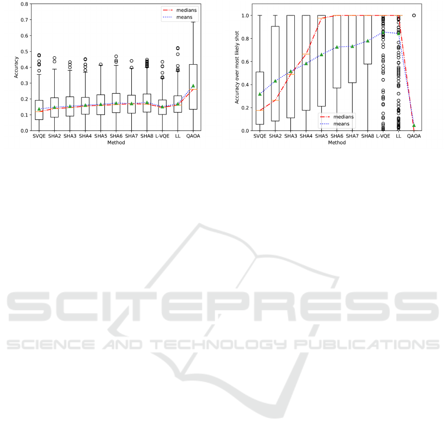
(a) Ratio of correct solutions. (b) Ratio of correct solutions of the most likely shot, averaged

over the last 2% of optimization steps.

Figure 2: Solution quality averaged over all graphs and circuit architectures for all considered approaches.

layer. Analogously to the previous evaluation on solu-

tion quality, we examine the overall accuracy as well

as the accuracy of the most likely shot, as displayed

in ﬁgure 3.

In terms of the overall accuracy (aside from

the QAOA), the combination of SHA8 and L-VQE

achieve the best results with a median accuracy

improvement of 35.5% against the standard VQE

(SVQE). This reveals a powerful synergy of combin-

ing SHA and L-VQE, as L-VQE performs worse than

LL when not coupled with SHA, but does so for their

hybrid variants. Overall the SHA+L-VQE hybrid out-

performs the previous empirical state-of-the-art VQE

approach (i.e., LL), by 5% in the mean. Examining

the results for the most likely shot, displayed in ﬁg-

ure 3b, we can see that the SHA+L-VQE hybrid also

performs the best overall, while improving 8.31%

over the previous best mean result (L-VQE). Interest-

ingly, the SHA+LL hybrid does only perform slightly

better than SHA (1.63%), but is worse than LL in this

metric. While the exact reasons for this performance

difference remain unclear based on the conducted ex-

periments, this shows that hybrid approaches do not

automatically improve the overall performance, but

can also even have negative effects on it.

6.4 Time Complexity

Aside from solution quality, the training duration is

a crucial performance indicator in practice. The less

optimization steps are needed, the faster the training

process in practice (i.e., when considering a similar

amount of parameters). The similarity in the num-

ber of parameters is important, because the quantum

gradient calculation scales linearly in this entity (see

section 2.1). As the actual number of concurrently

trained parameters is generally smaller in the layer-

wise approaches, this must be accounted for in an ex-

act runtime analysis. On average, our implementation

of LL trains only about half the number of parame-

ters in the full PQC, while L-VQE trains roughly

/3.

As the circuit depth also changes in layerwise learn-

ing approaches (and with that, the time needed to exe-

cute the circuits), this too inﬂuences the training time

complexity. Using our choice of hyperparameters, LL

executes

/4 of the full PQC on average, while L-VQE

only executes

/3.

However, due to the small absolute number of pa-

rameters and layers in our setting, we softly neglect

these complicating factors and inspect the raw dif-

ference in the number of optimization iterations as

displayed in ﬁgure 4. When comparing SHA to the

standard VQE, we observe a close to doubled number

of optimization iterations, which indicates, that the

signiﬁcant improvement in solution quality comes at

the cost of longer training time. However, real world

applications exist, in which the better achievable so-

lution quality outweighs the increase in runtime, as,

e.g., when benchmarking for the best possible perfor-

mance of a given VQE while aiming to show early

quantum advantage on a given QPU. Following the

considerations above, L-VQE and LL will have faster

wallclock times than SHA, even though they are on

par in the number of optimization iterations. For the

hybrid approaches, a signiﬁcant increase in runtime

can be observed, limiting their practical use cases in

spite of the qualitative improvements. When compar-

ing the SHA+LL hybrid to the SHA+L-VQE hybrid,

it becomes apparent that the approach with the bet-

ter solution quality (SHA+L-VQE) also trains faster,

which indicates, that the parameter landscape is eas-

ier to navigate through. Finally, it has to be ac-

knowledged, that a comparison of the VQE-based ap-

proaches to the QAOA baseline is especially hard,

ICAART 2024 - 16th International Conference on Agents and Artiﬁcial Intelligence

106

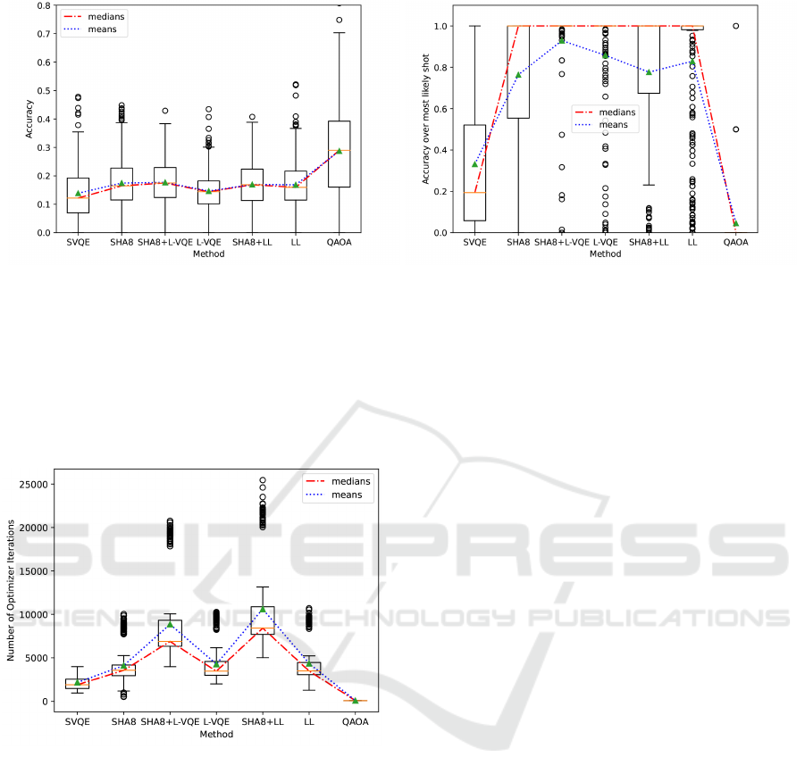
(a) Ratio of correct solutions. (b) Ratio of correct solutions of the most likely shot, averaged

over the last 3% of optimization steps.

Figure 3: Solution quality averaged over all graphs and circuit architectures when combining different approaches.

since QAOA’s PQC only has six parameters, acceler-

ating the optimization routine immensely. Neverthe-

less, this even underscores, the tremendously faster

trainability of the QAOA, at least in the regime of

short PQCs.

Figure 4: Number of optimization iterations.

7 DISCUSSION

These empirical ﬁndings display a valuable counter-

part to the ongoing theoretical efforts towards charac-

terizing the reasons for barren plateaus. This is partic-

ularly relevant, as current theoretical approaches as-

sume speciﬁc mathematical requirements for the cir-

cuit structure, the initial state and the measurement

operator, that are not necessarily given in practice

(Ragone et al., 2023). While the constraint that the

initial states or observables must lie in the circuit’s

Lie algebra (Ragone et al., 2023) has recently been

relaxed by focusing on matchgate circuits (Diaz et al.,

2023), results for arbitrary circuits are still to be ex-

plored. It is even possible that our results are no arti-

fact of locality, but rather an even deeper underlying

phenomenon (possibly generalized globality as intro-

duced in (Diaz et al., 2023)). Nevertheless, our ﬁnd-

ings support further research in this direction, as they

represent additional evidence towards the exploration

of the inﬂuence of the cost function on trainability.

8 CONCLUSION

The goal of this contribution was the development of

a novel quantum learning method, that facilitates the

parameter training for VQEs. Stemming on the fact

that increased locality in the cost function decreases

the risk of encountering vanishing gradients, we pro-

posed the sequential Hamiltonian assembly (SHA)

technique, that iteratively approximates the possibly

global cost function by assembling it from its local

components. In our experiments, we showed that our

approach improves the mean solution quality of the

standard VQE approach by 29.99% and outperforms

the empirical state of the art Layer-VQE by 5.12%

in certain applications. This demonstrates a prove of

principle and motivates further research on parame-

ter training approaches, that iteratively approximate

the original cost function to guide the learning pro-

cess. To extend this case study analysis of our ap-

proach, other problems beyond graph coloring should

be tested. An interesting candidate might be Max-

Cut, as it also offers a graph structure, allowing to ex-

amine the performance the proposed nodewise assem-

bly strategy. Beyond this, exploring new strategies for

graph and non-graph problems motivates future work.

As SHA slightly increases the wallclock training time

in its evaluated form, a more extensive hyperparame-

Improving Parameter Training for VQEs by Sequential Hamiltonian Assembly

107

ter search should be conducted to explore better qual-

ity/time tradeoffs. Having seen that combinations of

existing layerwise learning approaches with SHA can

increase the solution quality even further, gathering

more information on their interplay might open up

new approaches of quantum learning methods that

are especially targeted towards attacking multiple is-

sues of vanishing gradients concurrently, as, in our

case locality and expressiveness. In conclusion, our

contribution uncovers a new, locality based, approach

towards efﬁciently learning parameters in parameter-

ized quantum circuits.

ACKNOWLEDGEMENTS

This paper was partially funded by the German Fed-

eral Ministry for Economic Affairs and Climate Ac-

tion through the funding program "Quantum Comput-

ing – Applications for the industry" based on the al-

lowance "Development of digital technologies" (con-

tract number: 01MQ22008A).

REFERENCES

Aharonov, D., van Dam, W., Kempe, J., Landau, Z., Lloyd,

S., and Regev, O. (2004). Adiabatic quantum compu-

tation is equivalent to standard quantum computation.

In Proceedings of the 45th Annual IEEE Symposium

on Foundations of Computer Science, FOCS ’04, page

42–51, USA. IEEE Computer Society.

Albash, T. and Lidar, D. A. (2018). Demonstration of a scal-

ing advantage for a quantum annealer over simulated

annealing. Phys. Rev. X, 8:031016.

Bansal, N. (2014). New Developments in Iterated Round-

ing (Invited Talk). In Raman, V. and Suresh, S. P., ed-

itors, 34th International Conference on Foundation of

Software Technology and Theoretical Computer Sci-

ence (FSTTCS 2014), volume 29 of Leibniz Inter-

national Proceedings in Informatics (LIPIcs), pages

1–10, Dagstuhl, Germany. Schloss Dagstuhl–Leibniz-

Zentrum fuer Informatik.

Bengio, Y., Lamblin, P., Popovici, D., and Larochelle, H.

(2006). Greedy layer-wise training of deep networks.

In Schölkopf, B., Platt, J., and Hoffman, T., editors,

Advances in Neural Information Processing Systems,

volume 19. MIT Press.

Blekos, K., Brand, D., Ceschini, A., Chou, C.-H., Li, R.-

H., Pandya, K., and Summer, A. (2023). A review on

quantum approximate optimization algorithm and its

variants.

Born, M. and Fock, V. (1928). Beweis des Adiabatensatzes.

Zeitschrift für Phys., 51(3):165–180.

Bradley, D. M. (2010). Learning in modular systems.

Carnegie Mellon University.

Campos, E., Nasrallah, A., and Biamonte, J. (2021). Abrupt

transitions in variational quantum circuit training.

Phys. Rev. A, 103:032607.

Cerezo, M., Arrasmith, A., Babbush, R., Benjamin, S. C.,

Endo, S., Fujii, K., McClean, J. R., Mitarai, K., Yuan,

X., Cincio, L., and Coles, P. J. (2021a). Variational

quantum algorithms. Nat. Rev. Phys., 3(9):625–644.

Cerezo, M., Sone, A., Volkoff, T., Cincio, L., and Coles,

P. J. (2021b). Cost function dependent barren plateaus

in shallow parametrized quantum circuits. Nature

communications, 12(1):1791.

Deutsch, D. and Jozsa, R. (1992). Rapid solution of prob-

lems by quantum computation. Proceedings of the

Royal Society of London. Series A: Mathematical and

Physical Sciences, 439(1907):553–558.

Diaz, N., García-Martín, D., Kazi, S., Larocca, M., and

Cerezo, M. (2023). Showcasing a barren plateau the-

ory beyond the dynamical lie algebra. arXiv preprint

arXiv:2310.11505.

Du, Y., Huang, T., You, S., Hsieh, M.-H., and Tao, D.

(2022). Quantum circuit architecture search for varia-

tional quantum algorithms. npj Quantum Inf., 8(1):62.

Farhi, E., Goldstone, J., and Gutmann, S. (2014). A quan-

tum approximate optimization algorithm.

Fontana, E., Herman, D., Chakrabarti, S., Kumar, N.,

Yalovetzky, R., Heredge, J., Sureshbabu, S. H., and

Pistoia, M. (2023). The adjoint is all you need: Char-

acterizing barren plateaus in quantum ansätze.

Gilbert, E. N. (1959). Random Graphs. The Annals of Math-

ematical Statistics, 30(4):1141 – 1144.

Glorot, X. and Bengio, Y. (2010). Understanding the difﬁ-

culty of training deep feedforward neural networks. In

Teh, Y. W. and Titterington, M., editors, Proceedings

of the Thirteenth International Conference on Artiﬁ-

cial Intelligence and Statistics, volume 9 of Proceed-

ings of Machine Learning Research, pages 249–256,

Chia Laguna Resort, Sardinia, Italy. PMLR.

Gomez, S., Hennart, J.-P., and Powell, M. J. D., editors

(1994). A Direct Search Optimization Method That

Models the Objective and Constraint Functions by

Linear Interpolation, pages 51–67. Springer Nether-

lands, Dordrecht.

Grover, L. K. (1996). A fast quantum mechanical algorithm

for database search. In Proceedings of the Twenty-

Eighth Annual ACM Symposium on Theory of Com-

puting, STOC ’96, page 212–219, New York, NY,

USA. Association for Computing Machinery.

Hagberg, A., Swart, P., and S Chult, D. (2008). Explor-

ing network structure, dynamics, and function using

networkx. Technical report, Los Alamos National

Lab.(LANL), Los Alamos, NM (United States).

Holmes, Z., Sharma, K., Cerezo, M., and Coles, P. J. (2022).

Connecting ansatz expressibility to gradient magni-

tudes and barren plateaus. PRX Quantum, 3:010313.

Huang, Y., Lei, H., and Li, X. (2020). An empirical study

of optimizers for quantum machine learning. In 2020

IEEE 6th International Conference on Computer and

Communications (ICCC), pages 1560–1566.

Joshi, N., Katyayan, P., and Ahmed, S. A. (2021). Eval-

uating the performance of some local optimizers for

ICAART 2024 - 16th International Conference on Agents and Artiﬁcial Intelligence

108

variational quantum classiﬁers. Journal of Physics:

Conference Series, 1817(1):012015.

Kashif, M. and Al-Kuwari, S. (2023). The impact of cost

function globality and locality in hybrid quantum neu-

ral networks on nisq devices. Machine Learning: Sci-

ence and Technology, 4(1):015004.

Knill, E., Ortiz, G., and Somma, R. D. (2007). Optimal

quantum measurements of expectation values of ob-

servables. Physical Review A, 75(1):012328.

Lanczos, C. (2012). The Variational Principles of Mechan-

ics. Dover Books on Physics. Dover Publications.

Liu, X., Angone, A., Shaydulin, R., Safro, I., Alexeev, Y.,

and Cincio, L. (2022). Layer vqe: A variational ap-

proach for combinatorial optimization on noisy quan-

tum computers. IEEE Transactions on Quantum En-

gineering, 3:1–20.

Lucas, A. (2014). Ising formulations of many np problems.

Frontiers in Physics, 2.

McClean, J. R., Boixo, S., Smelyanskiy, V. N., Babbush,

R., and Neven, H. (2018). Barren plateaus in quantum

neural network training landscapes. Nat. Commun.,

9(1):4812.

Mitarai, K., Negoro, M., Kitagawa, M., and Fujii, K.

(2018). Quantum circuit learning. Phys. Rev. A,

98:032309.

Nielsen, M. A. and Chuang, I. L. (2010). Quantum Com-

putation and Quantum Information: 10th Anniversary

Edition. Cambridge University Press.

Peruzzo, A., McClean, J., Shadbolt, P., Yung, M.-H., Zhou,

X.-Q., Love, P. J., Aspuru-Guzik, A., and O’Brien,

J. L. (2014). A variational eigenvalue solver on a pho-

tonic quantum processor. Nat. Commun., 5(1):4213.

Pirnay, N., Ulitzsch, V., Wilde, F., Eisert, J., and Seifert, J.-

P. (2023). An in-principle super-polynomial quantum

advantage for approximating combinatorial optimiza-

tion problems.

Ragone, M., Bakalov, B. N., Sauvage, F., Kemper,

A. F., Marrero, C. O., Larocca, M., and Cerezo, M.

(2023). A uniﬁed theory of barren plateaus for deep

parametrized quantum circuits.

Sack, S. H., Medina, R. A., Michailidis, A. A., Kueng, R.,

and Serbyn, M. (2022). Avoiding barren plateaus us-

ing classical shadows. PRX Quantum, 3:020365.

Schuld, M., Bergholm, V., Gogolin, C., Izaac, J., and Killo-

ran, N. (2019). Evaluating analytic gradients on quan-

tum hardware. Phys. Rev. A, 99:032331.

Schuld, M., Sweke, R., and Meyer, J. J. (2021). Effect

of data encoding on the expressive power of varia-

tional quantum-machine-learning models. Phys. Rev.

A, 103:032430.

Sim, S., Johnson, P. D., and Aspuru-Guzik, A. (2019a).

Expressibility and entangling capability of parame-

terized quantum circuits for hybrid quantum-classical

algorithms. Advanced Quantum Technologies,

2(12):1900070.

Sim, S., Johnson, P. D., and Aspuru-Guzik, A. (2019b).

Expressibility and entangling capability of parame-

terized quantum circuits for hybrid quantum-classical

algorithms. Advanced Quantum Technologies,

2(12):1900070.

Skolik, A., McClean, J. R., Mohseni, M., van der Smagt, P.,

and Leib, M. (2021). Layerwise learning for quantum

neural networks. Quantum Mach. Intell., 3(1):5.

Stilck França, D. and Garcia-Patron, R. (2021). Limitations

of optimization algorithms on noisy quantum devices.

Nature Physics, 17(11):1221–1227.

Tabi, Z., El-Safty, K. H., Kallus, Z., Hága, P., Kozsik, T.,

Glos, A., and Zimborás, Z. (2020). Quantum opti-

mization for the graph coloring problem with space-

efﬁcient embedding. In 2020 IEEE International

Conference on Quantum Computing and Engineering

(QCE), pages 56–62.

Uvarov, A. and Biamonte, J. D. (2021). On barren plateaus

and cost function locality in variational quantum al-

gorithms. Journal of Physics A: Mathematical and

Theoretical, 54(24):245301.

Wang, S., Fontana, E., Cerezo, M., Sharma, K., Sone, A.,

Cincio, L., and Coles, P. J. (2021). Noise-induced bar-

ren plateaus in variational quantum algorithms. Na-

ture communications, 12(1):6961.

Zdeborová, L. and Krz ˛akała, F. (2007). Phase transitions

in the coloring of random graphs. Phys. Rev. E,

76:031131.

Zhang, K., Liu, L., Hsieh, M.-H., and Tao, D. (2022). Es-

caping from the barren plateau via gaussian initializa-

tions in deep variational quantum circuits. In Koyejo,

S., Mohamed, S., Agarwal, A., Belgrave, D., Cho, K.,

and Oh, A., editors, Advances in Neural Information

Processing Systems, volume 35, pages 18612–18627.

Curran Associates, Inc.

Improving Parameter Training for VQEs by Sequential Hamiltonian Assembly

109