Stochastic Single-Allocation Hub Location Routing Problem for the

Design of Intra-City Express Systems

Yuehui Wu

, Hui Fang

, Ali Gul Qureshi

and Tadashi Yamada

College of Transportation Engineering, Dalian Maritime University, Dalian, 116026, Liaoning, China

Department of Urban Management, Graduate School of Engineering, Kyoto University, Kyoto, 615-8246, Japan

Keywords: Intra-City Express, Stochastic Single-Allocation Hub Location Routing Problem, Multi-Stage Recourse Model,

Sample Average Approximation.

Abstract: The paper concentrates on designing an intra-city express system in a practical environment. In the target

networks, flows of parcels are exchanged between branch offices via a less-than-truckload hub-and-spoke

network in a stochastic environment. Hub and vehicle capacities are considered, and the flows between all

pairs of branch offices are assumed to be stochastic variables. The problem is modelled as a multi-stage

recourse model, named capacitated single-allocation hub location routing problem with stochastic demands

(CSAHLRPSD). A sample average approximation (SAA) framework is proposed, in which two variants of

adaptive large neighbourhood search algorithms are used to solve the SAA problem and to calculate the

recourse cost. The SAA framework is tested on benchmark instances, proving that it can efficiently deal with

the CSAHLRPSD. Also, the results indicate that employing the CSAHLRPSD can cut the operation cost in

comparison with the deterministic model in the practical and stochastic environment.

1 INTRODUCTION

Express service network design is significant in urban

logistics management as it can help reduce operation

costs and improve service levels. With the

development of e-commerce, intra-city express has

become an increasingly essential segment in urban

logistics systems. As a result, various cargo

companies are offering “delivery within the same day

in the city service”, “next day delivery service”, or

“delivery within 24 hours service”, e.g., SF Express,

Yamato Transport, Japan Post, and so on. For these

companies, how to satisfy the intra-city express

requests in a practical environment via a cost-efficient

way arises as an important issue. Moreover, this issue

is also significant for the urban management

department, as the delivery of intra-city expresses has

caused various social problems, e.g., traffic jams, air

pollution, and so on (Zhao et al., 2019).

In this study, we focus on the design of an intra-

city express system in a practical environment.

Parcels are transported from the origin branch offices

https://orcid.org/0000-0002-1755-3360

https://orcid.org/0000-0002-2832-2015

https://orcid.org/0009-0005-9937-951X

to the destination branch offices, resulting a many-to-

many distribution system. As the parcel and mail

flows are usually less-than-truckload (LTL), it is very

costly to link them directly, both from the economic

and social points of view (Gelareh & Nickel, 2011;

Sun, 2013). Instead, one method is to use the network

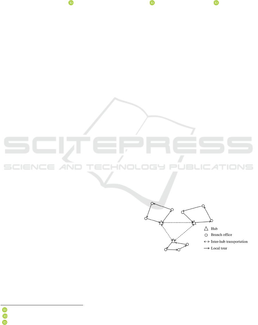
shown in Figure 1 to realize the flow exchange.

Figure 1: Hub-and-spoke network for intra-city express

systems.

This network is a variant of hub-and-spoke

networks specially designed for LTL transportation.

The hubs and branch offices are connected by local

tours instead of direct links, which is generally very

Wu, Y., Fang, H., Qureshi, A. and Yamada, T.

Stochastic Single-Allocation Hub Location Routing Problem for the Design of Intra-City Express Systems.

DOI: 10.5220/0012311900003639

Paper published under CC license (CC BY-NC-ND 4.0)

In Proceedings of the 13th International Conference on Operations Research and Enterprise Systems (ICORES 2024), pages 82-91

ISBN: 978-989-758-681-1; ISSN: 2184-4372

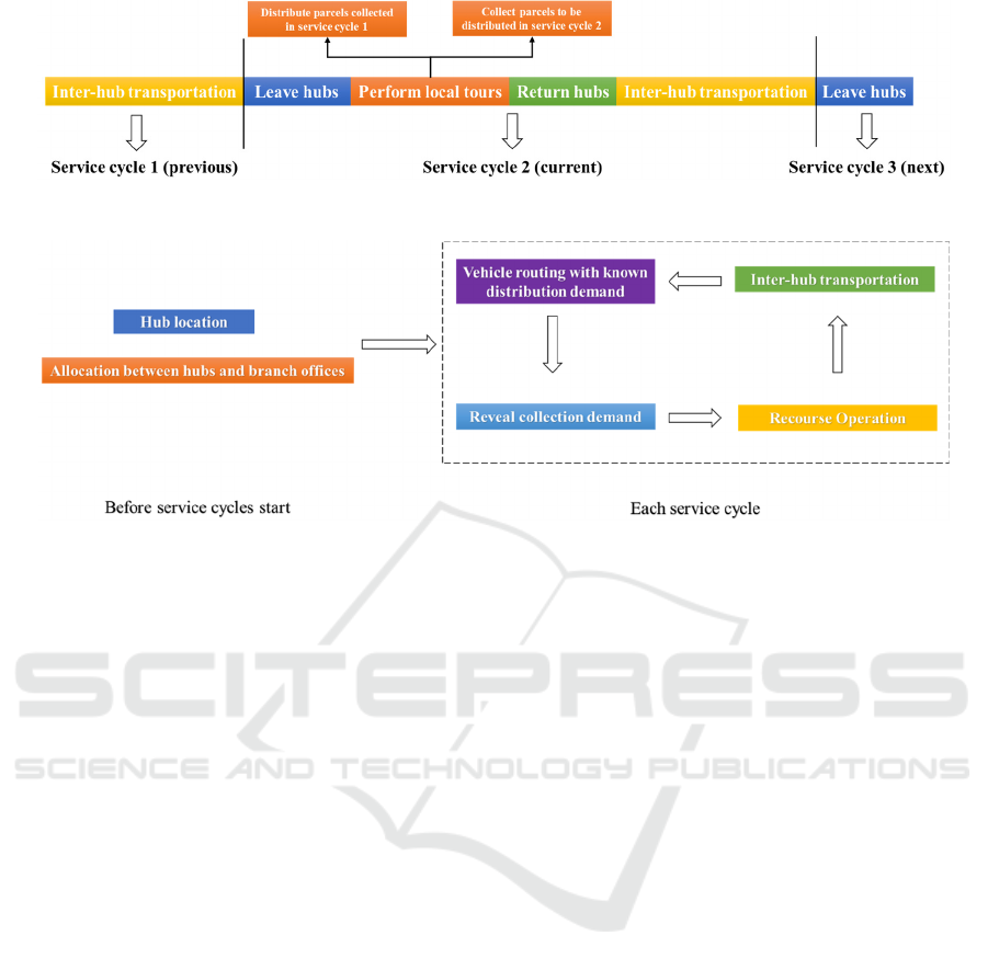
Figure 2: Hub-and-spoke network for intra-city express systems.

Figure 3: Stochastic decision process for intra-city express systems.

expensive (Kartal et al., 2017; Alumur et al., 2020).

The parcels are picked up at the origin branch

offices, sorted in the first hub, possibly transported to

the second hub, and delivered to the destination

branch offices. Moreover, the collection and

distribution processes are conducted at the same time

along local tours.

Branch offices usually do not own enough sorting

resources (e.g., labour, machines, spaces, and so on).

Therefore, parcels are collected in a mixed status and

have to be sorted based on their destinations in hubs

for further delivery. Consequently, the flow cannot be

exchanged directly, even along the same local tour.

More specifically, in the current service cycle (for

example, this morning), each vehicle leaves its

corresponding hub and traverses a subset of branch

offices, while distributing the parcels collected in the

previous service cycle (for example, yesterday

morning) and collecting the parcels to be distributed

in the next service cycle (for example, tomorrow

morning), i.e., the service system is a warmed-up

transportation system. Furthermore, inter-hub

transportation is conducted after the vehicles return to

the hubs (for example, at night). The whole procedure

is illustrated in Figure 2. Similar settings have been

applied in various studies related to the intra-city

express system design (such as in Sun, 2013; Karimi,

2018; Wu et al., 2023).

Based on the above descriptions, one can find that

the main decisions of the planning problem for the

referred system include hub location, allocation

between branch offices and hubs, and vehicle routing,

which should be resolved jointly. Moreover, the

following three practical conditions are considered:

(i) Capacity. Capacitated hubs and vehicles

should be employed due to the limitation of land

resources and the limitation of the use of large-

volume trucks in urban areas.

(ii) Single-allocation. In practical applications,

each branch office is usually served by precisely one

hub, as branch offices generally do not have enough

sort capacities.

(iii) Stochastic demand. The express company

might not know the parcel flows beforehand. For

instance, business activities might result in the

uncertainty of parcel flows, i.e., the intra-city express

demands are stochastic rather than deterministic. One

natural process to deal with the uncertainty is that the

hub location and allocation between hubs and branch

offices are decided before any random variable is

revealed (before service cycles start) since changing

these decisions for a warmed-up system is expensive.

In each service cycle, the vehicle routing is

determined with known distribution demand (since

these parcels have been collected in the previous

service cycle) and unknown collection demand.

Finally, recourse operations and inter-hub

transportation are conducted to finish the distribution

procedure. This process is shown in Figure 3.

With these considerations, we propose the

planning problem for the intra-city express system,

named capacitated single-allocation hub location

Stochastic Single-Allocation Hub Location Routing Problem for the Design of Intra-City Express Systems

routing problem with stochastic demand

(CSAHLRPSD), belonging to the field of the hub

location routing problem (HLRP). This problem has

been applied to the design of various many-to-many

systems, such as postal service systems (Bostel et al.,

2015), communication systems (Catanzaro et al.,

2015), ship cargo systems (Fontes & Goncalves,

2021), and so on. Please find more details of the

HLRP in Section 2.

The main contributions lay in three points: i) A

multi-stage recourse model is introduced to formulate

the CSAHLRPSD, which models the HLRP with

stochastic demand for the first time. ii) A sample

average approximation (SAA) framework, which is

embedded with two variants of the adaptive large

neighbourhood search (ALNS) algorithm, is

introduced as the solution approach. iii) Numerical

experiments are performed to prove the proposed

framework’s efficiency.

The remainder of the paper is structured as

follows: Section 2 reviews the HLRP and compares

our study with the existing ones. Section 3 defines the

CSAHLRPSD via a multi-stage recourse model.

Section 4 provides the solution methodology, whose

efficiency is tested in Section 5. Finally, Section 6

concludes the study.

2 LITERATURE REVIEW

This section mainly reviews the works on the single-

allocation hub location routing problem (SAHLRP),

which is closely concerning to the CSAHLRPSD.

Nagy and Salhi (1998) first proposed the SAHLRP

with route length constraints to limit working hours.

They proposed an integer linear programming

formulation for this problem and utilised a locate

first–route second heuristic algorithm to solve it on a

single instance with 249 clients.

So far, most studies related to the SAHLRP have

concentrated on postal service networks, where the

collection and distribution processes usually

coincide. Bostel et al. (2015) focused on an SAHLRP

where the length of each vehicle route is constrained

by a maximum number of visited clients. A memetic

algorithm (MA) was introduced to solve instances

with up to 100 clients. Kartal et al. (2017)

investigated the operational characteristics of a

leading cargo company in Turkey. Three variants of

formulations were introduced, and a multi-start

simulated annealing algorithm and an ACO algorithm

were introduced to solve the problem. Numerical

results indicated that the proposed algorithms could

find high-quality solutions for instances with up to

200 nodes in reasonable computational time. Karimi

(2018) studied a capacitated SAHLRP with

simultaneous pickup and delivery for a warmed-up

postal system. The study introduced a polynomial-

sized mixed integer programming formulation and

several valid inequalities. Moreover, a tabu-search-

based heuristic was proposed to solve the problem.

The results from computational tests showed that the

proposed valid inequalities and algorithm worked

well for their model.

The pickup and delivery process can be distinct

for logistical or scheduling reasons, e.g., the case for

general freight forwarders. Sun (2015) investigated a

problem similar to the one in Sun (2013), in which

pickup and deliveries were assumed to be distinct. An

endosymbiotic evolutionary algorithm was

developed, simultaneously solving hub location and

vehicle routing problems. The algorithm’s

performance was tested on 20 instances with 100 and

200 customers. Experimental results showed that the

proposed algorithm could be used for supply-chain

network planning. More recently, Yang et al. (2019)

investigated the capacitated SAHLRP with distinct

collection and delivery processes. Moreover, they

proposed a new MILP model and developed a

memetic algorithm (MA) to solve larger-sized

problems. Numerical experiments showed that the

MA could find high-quality solutions in acceptable

computational time.

Most studies have employed heuristic algorithms

(Danach et al., 2019; Ratli et al., 2020; Pandiri &

Singh, 2021), and there are only a few attempts to

solve the problem exactly. de Camargo et al. (2013)

introduced a new SAHLRP model with simultaneous

collections and distributions. They assumed that a

fixed cost was imposed upon the hubs and vehicles.

Moreover, they decomposed the problem into two

subproblems: a transportation problem and a

feasibility problem. Then the problem was optimally

solved by a tailored Benders decomposition

algorithm. The results were compared to the CPLEX

solver, proving that this method was able to find

optimal solutions for instances with 100 clients.

Later, Rodriguez-Martin et al. (2014) investigated a

variant of SAHLRP in which a cyclical path

connected the uncapacitated hubs. In the problem,

each cluster of clients and assigned hub was

connected by precisely one local route cycle.

Furthermore, the number of visited clients of each

local route cycle is limited as a length constraint. The

problem was solved by a branch-and-cut algorithm.

Wu et al. (2023) provided a branch-and-price-and-cut

algorithm to solve the capacitated SAHLRP, which

were tested on benchmark instances. Numerical

ICORES 2024 - 13th International Conference on Operations Research and Enterprise Systems

results proved that the branch-and-price-and-cut

algorithm could efficiently deal with the capacitated

SAHLRP.

All the above works have focused on the

deterministic HLRPs, and there is only one work on

the stochastics HLRP. Mohammadi et al. (2013)

investigated a multi-objective chance-constrained

model of a stochastic green HLRP. In their problem,

stochastic travel time and service time were

considered. A multi-objective invasive weed

optimisation was introduced to solve the problem,

which was then compared with other multi-objective

algorithms on randomly generated instances.

As reviewed above, stochastic HLRP-related

literature is extremely limited. Our study is the first

one to investigate the HLRP with stochastic demands.

Moreover, our work is the first attempt to model the

stochastic HLRP via the recourse model.

3 MODEL FORMULATION

The CSAHLRPSD is defined on a complete

graph 𝐺 =

(

𝑉,𝐴

)

, in which 𝑉 and 𝐴 are vertex set

and edge set, respectively. Vertex set 𝑉 consists of

potential hub set 𝐻 and client (branch office) set 𝐶,

while edge set 𝐴 consists of edges between all

vertices. For each pair of clients 𝑖 ∈ 𝐶 and 𝑗 ∈

𝐶, 𝑑



represents the flow to be transported from 𝑖 to

𝑗 through local tours and hubs, which is assumed to

be a random variable with known and independent

distribution. Without loss of the generality, we

assume that all realizations of 𝑑



are greater than 0

and they do not exceed the vehicle capacity.

Moreover, the collection demand and distribution

demand of client 𝑖 ∈ 𝐶 is denoted as 𝑂



∑

𝑑

∈

and 𝐷



∑

𝑑

∈

, respectively.

Each potential hub has a capacity 𝑄



and a fixed

cost 𝐹



. As in Ernst and Krishnamoorthy (1999), Hu

et al. (2021) and Ghaffarinasab (2022), it is assumed

that only receiving flows from clients consumes hub

capacity since parcels are generally sorted in the

origin hubs and then transported to destination hubs

without further sorting operations. Local tours are

operated by an unlimited fleet of identical vehicles,

and each vehicle is associated with a capacity 𝑞 and a

fixed cost 𝑓. Furthermore, inter-hub transportation is

assumed to be realised by an unlimited fleet of

identical trucks, and there is no capacity limitation

and fixed cost of the trucks.

Each edge

(

𝑖,𝑗

)

∈𝐴 is addressed with a

nonnegative travel distance 𝑐



, satisfying the triangle

inequality. Local tour cost is dependent on the sum of

travel distances of the travelled edges, while inter-hub

transportation cost is calculated based on travel

distances and transferred flows (Karimi, 2018; Yang

et al., 2019). In addition, the unit inter-hub

transportation cost (¥/km.t) and unit local tour cost

(¥/km) are denoted as 𝛼 and 𝛽, respectively.

The CSAHLRPSD belongs to the field of

stochastic programming, which is generally

formulated by chance-constrained models and

recourse models. Based on the descriptions in Section

1, we model the CSAHLRPSD via a multi-stage

recourse model as follows:

i) In the first stage, the hub locations and the

allocation between clients and hubs (long-term

decisions) are determined before the random

variables (𝑑



|𝑖,𝑗 ∈ 𝐶) are realised.

ii) Then, in the second stage, the flows to be

delivered to each client 𝑖 ∈ 𝐶 (𝑑



|𝑗 ∈ 𝐶) are revealed

first (since these parcels have been collected in the

previous service cycle, as shown in Section 1),

forming the distribution demands (𝐷



|𝑖 ∈ 𝐶). After

the distribution demands are known, the vehicles are

routed to link the hubs and clients (short-term

decisions) before knowing the collection demands

(𝑂



|𝑖 ∈ 𝐶).

iii) In the third stage, the collection demands are

revealed, and a predetermined recourse policy is

applied when a failure occurs. The classical recourse

policy is employed, in which the vehicles return to the

hub, drop off the collected parcels, and continue their

planned route at the point of failure. Furthermore, if

the total collection demand assigned to a hub exceeds

its capacity due to uncertainty, a penalty cost must be

paid, representing the overwork cost. The unit

overwork cost is expressed as ω. Note that the inter-

hub transportation costs are also calculated in this

stage.

In other words, after the hub location and the

allocation between hubs and clients are determined, a

VRPSDSP is solved for each installed hub and the

clients assigned to it. Although these VRPSDSPs

need to be solved multiple times for all the service

cycles, we only model them once for simplicity, and

the fixed costs are distributed into each service cycle

to make long-term and short-term costs comparable.

For each edge (𝑖,𝑗) ∈ 𝐴, 𝑥



is a binary variable

equal to 1 if there is a vehicle travelling directly from

vertex 𝑖 to vertex 𝑗. 𝑧



(𝑖∈𝐶,𝑘∈𝐻) is a binary

variable equal to 1 if client 𝑖 is allocated to hub 𝑘. For

each vertex 𝑖 ∈ 𝑉, let 𝑣



be the delivery load on the

vehicle just after having served vertex 𝑖. 𝑏



is a binary

variable equal to 1 if potential hub 𝑘 ∈ 𝐻 is open.

Moreover, 𝑦



denotes the fraction flow from

client 𝑖 ∈ 𝐶 to client 𝑗 ∈ 𝐶 passing hub 𝑘 ∈ 𝐻 and

Stochastic Single-Allocation Hub Location Routing Problem for the Design of Intra-City Express Systems

hub 𝑙 ∈ 𝐻. Finally,

𝑒



denotes the overwork load of

hub 𝑘 ∈ 𝐻.

The CSAHLRPSD is modelled as (1)-(21), in

which 𝑄



(

𝒃,𝒛,𝝃

)

and 𝑄



(

𝒙,𝒃,𝒛,𝝃

)

are the optimal

value of the second stage problem and the third stage

problem. Random vector 𝝃 contains the flow 𝑑



to be

transported from client 𝑖 ∈ 𝐶 to 𝑗 ∈ 𝐶.

𝑆𝑡𝑎𝑔𝑒 1 𝑚𝑖𝑛  𝐹



𝑏



∈

+𝐸[𝑄



(

𝒃,𝒛,𝝃

)

]

(1)

𝑠.𝑡.𝑧



∈

=1∀𝑖∈𝐶

(2)

𝑧



≤𝑏



∀𝑖 ∈ 𝐶,𝑘 ∈ 𝐻

(3)

𝑧



∈



0,1



∀𝑖 ∈ 𝐶, 𝑘 ∈ 𝐻

(4)

𝑏



∈



0,1



∀𝑘 ∈ 𝐻

(5)

Objective function (1) minimises the operation

cost, consisting of the hub fixed cost and expected

recourse cost. Constraint (2) guarantees the single-

allocation between clients and hubs. Only open hubs

can serve clients, which is ensured by Constraint (3).

Constraints (4) and (5) are variable domains.

𝑆𝑡𝑎𝑔𝑒 2 𝑄



(

𝒃,𝒛,𝝃

)

=min𝑓𝑥



∈∈

+𝛽𝑐



𝑥



∈∈

+𝐸[𝑄



(

𝒃,𝒛,𝒙, 𝝃

)

]

(6)

𝑠.𝑡.  𝑥



=1∀𝑖∈𝐶

∈

(7)

𝑥



=𝑥



∈

∀𝑖 ∈ 𝑉

∈

(8)

𝑥



≤𝑧



∀𝑖 ∈ 𝐶, 𝑘 ∈ 𝐻

(9)

𝑥



≤𝑧



∀𝑖 ∈ 𝐶, 𝑘 ∈ 𝐻

(10)

𝑥



+𝑧



+𝑧



∈

≤2 ∀𝑖∈𝐶,

𝑗

≠𝑖∈𝐶,𝑘∈𝐻

(11)

𝑣



−𝐷



+𝑞(1−𝑥



)≥𝑣



∀𝑖 ∈ 𝑉,

𝑗

≠𝑖∈𝐶

(12)

𝑣



≤𝑞 ∀𝑖∈𝑉

(13)

𝑥



∈



0,1



∀𝑖 ∈ 𝑉,

𝑗

∈𝑉

(14)

𝑣



≥ 0 ∀𝑖 ∈ 𝑉

(15)

Objective function (6) minimises the vehicle fixed

cost, local tour cost, and expected recourse cost. Each

client should be visited by exactly one vehicle, which

is guaranteed by Constraint (7). Constraint (8)

balances the vehicle flow at each vertex. Constraints

(9)-(11) link the allocation variables with routing

variables. Constraint (12) describes the delivery load

on vehicles. Vehicle capacity constraints are imposed

via Constraint (13). Decision variables are defined by

Constraints (14)-(15).

𝑆𝑡𝑎𝑔𝑒 3 𝑄



(

𝒃,𝒛,𝒙,𝝃

)

=𝑚𝑖𝑛𝑅

(

𝒙,𝝃

)

+𝜔𝑒



∈

+𝛼𝑑



𝑐



𝑦



∈∈∈∈

(16)

𝑠.𝑡.𝑦



=𝑧



∀𝑖 ∈ 𝐶,

𝑗

∈𝐶,𝑘∈𝐻

∈

(17)

𝑦



=𝑧



∀𝑖 ∈ 𝐶,

𝑗

∈𝐶,𝑙∈𝐻

∈

(18)

𝑒



≥ 𝑑



𝑦



−𝑄



∈∈∈

∀𝑘∈𝐻

(19)

0≤𝑦



≤1∀𝑖∈𝐶,

𝑗

∈𝐶,𝑘∈𝐻,𝑙∈𝐻

(20)

𝑒



≥0∀𝑘∈𝐻

(21)

Objective function (16) optimises the realised

recourse cost (𝑅

(

𝒙,𝝃

)

) and overwork cost. Also, the

inter-hub transportation cost is calculated via the third

term of it. Constraints (17)-(18) correlate the flow

variables and allocation variables. Note that

Constraints (17)-(18), along with Constraints (9)-

(11), connect the allocation variables 𝒛 , flow

variables 𝒚, and routing variables 𝒙, ensuring the

proper network flow assignment. Overwork cost for

each hub 𝑘 ∈ 𝐻 is calculated via Constraint (19).

Constraints (20)-(21) are variable domains. Since

there is no simple way to formulate the computation

of 𝑅

(

𝒙,𝝃

)

via decision variables and linear

relationships (Laporte et al., 2002), we do not provide

a specific formulation here. However, one can find a

way to calculate its expectation in Laporte et al.

(2002) and Hernandez et al. (2019).

4 SOLUTION METHODOLOGY

4.1 Sample Average Approximation

The key to solving model (1)-(21) is calculating

𝐸[𝑄



(

𝒃,𝒛,𝝃

)

], which is very difficult even under a

discrete distribution. Thus, we present an SAA-based

approach to approximate 𝐸

[

𝑄



(

𝒃,𝒛,𝝃

)

]

. The SAA

approach is presented by Kleywegt et al. (2002),

whose principle is that sampling problems can

approximate the numerical expectation. A random

sample with size 𝑁 is generated first. Then the

CSAHLRPSD can be approximated as below:

𝑆𝐴𝐴 𝑃𝑟𝑜𝑏𝑙𝑒𝑚:𝑚𝑖𝑛  𝐹



𝑏



∈

𝑁

𝑄



(

𝒃,𝒛,𝝃

𝒏

)





(22)

s.t. (2)-(5)

(23)

ICORES 2024 - 13th International Conference on Operations Research and Enterprise Systems

The obtained solution is evaluated on a larger

sample with size 𝑁



( 𝑁



≫𝑁) by obtaining the

approximate SAA gap and the variance of the gap

estimator. If they are small enough, the solution is

accepted as the CSAHLRPSD’s solution. Otherwise,

the sample sizes should be increased. This process is

shown in Algorithm 1. In the algorithm, 𝑧





(

𝒃,𝒛

)

and 𝑧





(

𝒃,𝒛

)

denote the objective function values of

the solution

(

𝒃,𝒛

)

on scenario 𝜉



and sample 𝑁′,

respectively. We define “sufficiently small” as:

𝜖

,



(

𝒃,𝒛

)

/𝑧





(

𝒃,𝒛

)

≤3% and 𝜎



,



(

𝒃,𝒛

)

𝑧





(

𝒃,𝒛

)

≤5%.

Input: the number of SAA replications 𝑀 and the sample

sizes, 𝑁 and 𝑁



(𝑁



≫𝑁)

Step 1:

For 𝑚 = 1,2,…,𝑀, do:

Generate a sample with size 𝑁 by realising 𝜉





, 𝜉





, …, 𝜉





;

Solve the SAA to get the solution

(

𝒃,𝒛

)



and the objective

value 𝑧





;

Obtain the statistical lower-bound 𝑧







∑

𝑧













;

Obtain the variance of the statistical lower-bound 𝜎



(

𝑧



)



()

∑

(𝑧







−𝑧



)









;

Generate a sample with size 𝑁



and get the upper-

bound 𝑧





(

𝒃,𝒛

)



and a estimate of variance of upper-bound

𝜎







(

𝒃,𝒛

)









(



)

∑

(𝑧





(

𝒃,𝒛

)



−𝑧





(

𝒃,𝒛

)



)









;

Select the solution

(

𝒃,𝒛

)

with best 𝑧





(

𝒃,𝒛

)

then ontain the

SAA gap 𝜖

,



(

𝒃,𝒛

)

=𝑧





(

𝒃,𝒛

)

−𝑧



;

Calculate the variance of the SAA gap 𝜎



,





(

𝒃,𝒛

)

𝜎



(

𝑧



)

+𝜎







(

𝒃,𝒛

)

;

If 𝜖

,



(

𝒃,𝒛

)

and 𝜎



,





(

𝒃,𝒛

)

sufficiently small:

Go to Step 3;

End

Step 2:

If 𝜖

,



(

𝒃,𝒛

)

and 𝜎



,





(

𝒃,𝒛

)

not sufficiently small:

Increase the sample size 𝑁 and/or 𝑁



and go to Step 1

End

Step 3: Output:

(

𝒃,𝒛

)

Stop

Algorithm 1: SAA algorithm.

The SAA problem is a special variant of the HLP.

More complex, calculating 𝑄



(

𝒃,𝒛,𝝃

)

is NP-hard

even when 𝑏



(𝑘 ∈ 𝐻) and 𝑧



(𝑖∈𝐶,𝑘∈𝐻) are

fixed. As a result, two ALNS algorithms are

introduced as the solution approach for solving the

SAA problem and getting 𝑄



(

𝒃,𝒛,𝝃

)

, respectively.

These two algorithms are designed according to the

one used by Wu et al. (2022), which has been proven

to solve the HLRP efficiently. For notation simplicity,

we name them ALNS-SAA and ALNS-RECOURSE,

respectively.

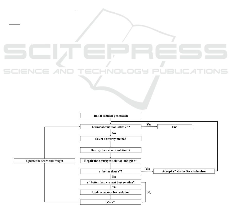
4.2 Adaptive Large Neighbourhood

The ALNS algorithm has been successful in solving

various routing problems, e.g., vehicle routing

problem, pickup and delivery problem, location

routing problem, and so on. We follow the procedure

in Ropke and Pisinger (2006) to present the ALNS-

SAA and ALNS-RECOURSE: In each iteration, a

destroy method removes several clients from the

current solution, and then a repair method inserts

them into the destroyed solution to obtain a new

solution. Each method is associated with a weight and

is randomly selected based on their weights. The

weights are adjusted adaptively based on their

performance. The new solution is accepted is it is

Figure 4: ALNS algorithm

Stochastic Single-Allocation Hub Location Routing Problem for the Design of Intra-City Express Systems

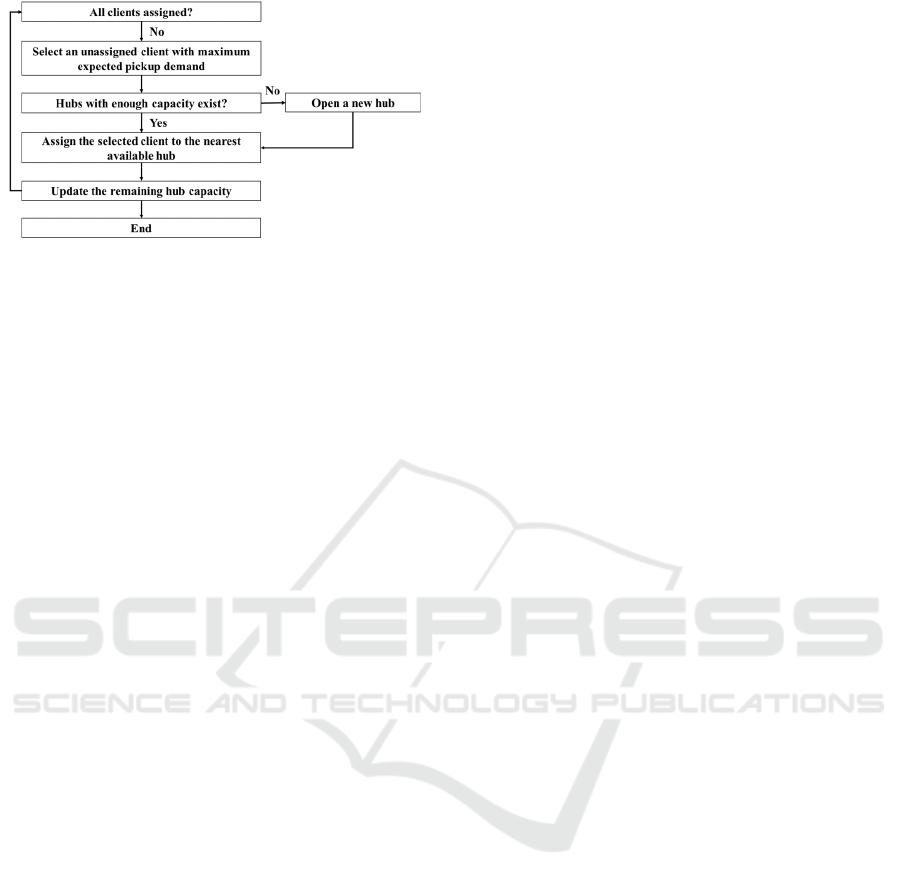
Figure 5: Greedy algorithm.

better than the current one. Otherwise, a simulated

annealing mechanism is applied to determine whether

the new solution is accepted. Although the ALNS-

SAA and ALNS-RECOURSE have the same

procedures, their destroy/repair methods and initial

solution generation methods are different, which will

be presented in Section 4.2.1 and Section 4.2.2.

Please refer to Wu et al. (2022) for the common parts

(e.g., weight adjustment, destroy/repair method

selection, and simulated annealing mechanism).

4.2.1 ALNS-SAA

a. Initial Solution Generation

We use the following greedy algorithm (Figure 5) for

the initial solution generation. The clients are

allocated to the nearest open hubs one-by-one. If such

hubs do not exist, a new hub is installed. The process

continues until all clients are assigned.

b. Destroy Method

Random Hub Removal: This method randomly

selects one open hub and closes it. All linked clients

are deleted from the current solution and added into

the client pool.

Worst Usage Hub Removal: This method closes

the open hub with the least utilisation ratio. All clients

allocated to it are deleted and added into the client

pool.

Random Hub Opening: This method randomly

selects one close hub and opens it. Then, several

clients are randomly selected, deleted from the

current solution, and then put in the client pool.

Random Allocation Change: This method aims

to optimise the allocation between clients and hubs.

The randomly-selected clients are deleted from the

current solution and inserted into the client pool.

Worst Allocation Removal: This method delates

some clients far from the hubs they are allocated to.

The distance is randomised and normalised to avoid

constantly selecting the same clients.

c. Repair Method

Greedy Insertion: The clients are inserted into

the solution randomly, one after the other, into the

position with minimum insertion cost.

4.2.2 ALNS-RECOURSE

a. Initial Solution Generation

The following nearest-neighbour algorithm

(Algorithm 2) is used to generate initial solutions for

calculating 𝑄



(

𝒃,𝒛,𝝃

)

For each open hub 𝑘:

While unlinked clients allocated to hub 𝑘 exist:

Initialise vertex 𝑣 = 𝑘

Initialize pickup capacity 𝑝=𝑞

Initialize delivery capacity 𝑑=𝑞

While available unrouted clients exist:

Select unrouted client 𝑖 nearest to 𝑣

𝑣=𝑖

𝑝=𝑝−𝐸[𝑂



],𝑑 = min

(

𝑝−𝑂



,𝑑−𝐷



)

End

Algorithm 2: Nearest-neighbour algorithm.

b. Destroy Method

Random Removal: This method chooses several

clients randomly and adds them into the client pool.

Worst Cost Removal: This method deletes some

clients far from the vertexs visited just before and

ahead of them.

Shaw Removal: This method aims to remove

clients similar to each other.

Random Route Removal: This method deletes a

randomly-selected route and adds its visited clients

into the client pool.

c. Repair Method

The same Greedy Insertion is used. However,

the clients can only be inserted into the routes

departing from their assigned hub.

5 NUMERICAL EXPERIMENTS

5.1 Instance Generation

The numerical experiments have been conducted on

the instances with up to 25 clients used in Wu et al.

(2023). These instances are generated from Australia

Post (AP) benchmark, and each instance is associated

with 5 potential hubs. In AP benchmark, two types of

capacities and fixed costs, tight (T) and loose (L), are

included. Hence, for each instance, four types of

ICORES 2024 - 13th International Conference on Operations Research and Enterprise Systems

Table 1: Experiment Results.

Instance

𝐹



𝐼𝑡𝑒 𝑇𝑖𝑚𝑒 𝐺𝑎𝑝



𝐶𝑜𝑣



Hub

𝐹



𝐺𝑎𝑝



10-L-L 222384.42 2 152.98 0.78 2.42 5 245590.46 9.45

10-L-T 241054.01 2 139.45 1.97 3.05 2,4 264116.68 8.73

10-T-L 248461.71 2 153.27 1.09 2.10 4,5 302806.87 17.95

10-T-T 281902.80 2 188.32 1.32 2.38 2,3,4 342478.48 17.69

15-L-L 287050.82 2 243.53 1.71 4.01 4,5 307109.76 6.53

15-L-T 332315.13 3 342.98 1.87 2.12 1,3 377309.28 11.93

15-T-L 348108.70 2 240.57 1.71 3.68 1,2,5 371482.83 6.29

15-T-T 382314.72 2 251.31 2.56 3.32 1,4 424999.28 10.04

20-L-L 333865.76 2 516.37 1.74 2.49 4,5 364298.63 8.35

20-L-T 351368.10 3 718.51 1.62 3.65 3,4 409825.32 14.26

20-T-L 392668.70 2 588.52 2.56 3.35 3,4,5 438775.19 10.51

20-T-T 428306.20 2 595.87 1.19 2.21 1,2,4 435075.15 1.56

25-L-L 346804.95 2 1011.23 2.05 1.70 2,5 372620.88 6.93

25-L-T 372854.75 2 1403.59 1.54 2.58 2,3 406846.89 8.36

25-T-L 415943.60 2 1236.84 1.63 4.43 2,3,4 427874.59 2.79

25-T-T 441345.67 2 1238.92 2.41 1.88 2,3,4 487703.49 9.51

problems (i.e., LL, LT, TL, and TT) can be created.

The used instances are named as N-Q-F, where 𝑁 ∈



10,15,20,25



denotes the number of clients,

and 𝑄 and 𝐹 indicate the type of hub capacity and

fixed cost (tight and loose), respectively. For

example, 15-L-L means an instance with 15 clients,

and its hub capacity and fixed cost are loose.

We have adjusted these instances and applied the

proposed SAA framework to them. The main

adjustments are:

(i) The flow 𝑑



of each pair of clients 𝑖 and

𝑗

(

𝑗≠𝑖

)

is assumed to be subject to a uniform

distribution [0.6𝑑





, 1.4𝑑





], in which 𝑑





is the value

provided by the generator.

(ii) Vehicle capacity and fixed cost were set as

850 and 3000 in all instances, respectively, ensuring

that each client could be served by a single vehicle.

The SAA framework is corded in Java, and a PC

with Intel i5-13600KF CPU and 32 GB RAM is used

to conduct the experiments.

5.2 Computation Results

In this section, the stochastic model and deterministic

model are compared. For the stochastic model, we

employ the SAA framework (𝑁=40,

𝑁′ = 2000,

𝑀=10) for each instance. For the deterministic

model, each instance is solved by the branch-and-

price-and-cut algorithm used in Wu et al. (2023), in

which the values of the random variables are set as

their mathematical expectations. After solving the

stochastic model and deterministic model, a new

sample with size 2000 (called evaluation sample) is

generated to compare their solutions’ qualities. The

comparison is concluded in Table 1. The definition of

the notations in it is presented below:

 𝐹



: the operation cost of the evaluation

sample of the SAA framework.

 𝐼𝑡𝑒: the number of SAA problems used to

achieve sufficiently small gap and variance.

 𝑇𝑖𝑚𝑒: computational times (second) for the

SAA framework.

 𝐺𝑎𝑝



: the SAA gaps.

 𝐶𝑜𝑣



: the coefficient of variation (COV)

of the SAA approximator.

 𝐹



: the operation cost of the evaluation

sample of the deterministic model.

 𝐺𝑎𝑝



: the gap between 𝐹



and 𝐹



It can be concluded in Table 1 that the SAA

framework dealt with the CSAHLRPSD adequately:

𝐺𝑎𝑝



(1.74% on average and 2.56% in the worst

Stochastic Single-Allocation Hub Location Routing Problem for the Design of Intra-City Express Systems

case) and 𝐶𝑜𝑣



(2.84% on average and 4.43% in

the worst case) were small. Moreover, in 14 of 16

instances, two SAA replications are needed to reach

the small-enough 𝐺𝑎𝑝



and 𝐶𝑜𝑣



, indicating that

the sample size is chosen adequately. Furthermore,

the column “Time” demonstrated that the SAA

framework was able to solve the CSAHLRPSD in

acceptable calculational times, and all instances were

solved in less than 1500s. These computational times

are acceptable as long-term decisions need to be

determined only once for each network. Furthermore,

for each service cycle, the short-term decisions can be

determined in a very short time. Finally, one can find

that considering stochastic factors can effectively cut

down the cost: the average 𝐺𝑎𝑝



is 9.43%, while the

best 𝐺𝑎𝑝



is 17.95%.

6 CONCLUSIONS

In this paper, we concentrated on the CSAHLRPSD

problem. The aim of the problem is to design an intra-

city express system in a practical environment.

Therefore, capacitated hubs and vehicles were

employed, and the flows were assumed to be

stochastic. The problem was formulated as a multi-

stage recourse model, and an SAA framework was

introduced to solve the problem. In the framework,

two variants of the ALNS algorithm were used to

solve the SAA problem and to calculate the recourse

cost. The proposed method was evaluated on the

benchmark instances, proving that the SAA

framework can solve the CSAHLRPSD in acceptable

computational times and that considering stochastic

factors can effectively decrease the operation cost (by

9.43% on average). Future studies include proposing

more efficient algorithms to calculate the recourse

cost and to apply the framework to more instances.

ACKNOWLEDGEMENTS

This work was supported by Japan Society for the

Promotion of Science (JSPS), Kakenhi (Grants-in-

Aid for ScientificResearch - C) [20K04739] and the

National Natural Science Foundation of China (Grant

No. 72301052).

REFERENCES

Alumur, S. A., Campbell, J. F., Contreras, I., Kara, B. Y.,

Marianov, V., & O’Kelly, M. E. (2021). Perspectives

on modeling hub location problems. European Journal

of Operational Research, 291(1), 1-17.

Bostel, N., Dejax, P., & Zhang, M. (2015). A model and a

metaheuristic method for the hub location routing

problem and application to postal services. 2015

International Conference on Industrial Engineering and

Systems Management (pp. 1383-1389). IEEE.

Catanzaro, D., Gourdin, E., Labbé, M., & Özsoy, F. A.

(2011). A branch-and-cut algorithm for the

partitioning-hub location-routing problem. Computers

& operations research, 38(2), 539-549.

Çetiner, S., Sepil, C., & Süral, H. (2010). Hubbing and

routing in postal delivery systems. Annals of

Operations research, 181(1), 109-124.

Danach, K., Gelareh, S., & Monemi, R. N. (2019). The

capacitated single-allocation p-hub location routing

problem: a Lagrangian relaxation and a hyper-heuristic

approach. EURO Journal on Transportation and

Logistics, 8(5), 597-631.

de Camargo, R. S., de Miranda, G., & Løkketangen, A.

(2013). A new formulation and an exact approach for

the many-to-many hub location-routing problem.

Applied Mathematical Modelling, 37(12-13), 7465-

7480.

Ebery, J., Krishnamoorthy, M., Ernst, A., & Boland, N.

(2000). The capacitated multiple allocation hub

location problem: Formulations and algorithms.

European journal of operational research, 120(3), 614-

631.

Ernst, A. T., & Krishnamoorthy, M. (1999). Solution

algorithms for the capacitated single allocation hub

location problem. Annals of operations Research, 86,

141-159.

Fontes, F. F. D. C., & Goncalves, G. (2021). A variable

neighbourhood decomposition search approach applied

to a global liner shipping network using a hub-and-

spoke with sub-hub structure. International Journal of

Production Research, 59(1), 30-46.

Gelareh, S., & Nickel, S. (2011). Hub location problems in

transportation networks. Transportation Research Part

E: Logistics and Transportation Review, 47(6), 1092-

1111.

Ghaffarinasab, N. (2022). Stochastic hub location problems

with Bernoulli demands. Computers & Operations

Research, 145, 105851.

Hernandez, F., Gendreau, M., Jabali, O., & Rei, W. (2019).

A local branching matheuristic for the multi-vehicle

routing problem with stochastic demands. Journal of

Heuristics, 25, 215-245.

Hu, Q. M., Hu, S., Wang, J., & Li, X. (2021). Stochastic

single allocation hub location problems with balanced

utilisation of hub capacities. Transportation Research

Part B: Methodological, 153, 204-227.

Karimi, H. (2018). The capacitated hub covering location-

routing problem for simultaneous pickup and delivery

systems. Computers & Industrial Engineering, 116, 47-

58.

Kartal, Z., Hasgul, S., & Ernst, A. T. (2017). Single

allocation p-hub median location and routing problem

with simultaneous pick-up and delivery. Transportation

ICORES 2024 - 13th International Conference on Operations Research and Enterprise Systems

Research Part E: Logistics and Transportation Review,

108, 141-159.

Kleywegt, A. J., Shapiro, A., & Homem-de-Mello, T.

(2002). The sample average approximation method for

stochastic discrete optimisation. SIAM Journal on

optimisation, 12(2), 479-502.

Laporte, G., Louveaux, F. V., & Van Hamme, L. (2002).

An integer L-shaped algorithm for the capacitated

vehicle routing problem with stochastic demands.

Operations Research, 50(3), 415-423.

Li, X., & Zhang, K. (2018). A sample average

approximation approach for supply chain network

design with facility disruptions. Computers & Industrial

Engineering, 126, 243-251.

Mohammadi, M., Razmi, J., & Tavakkoli-Moghaddam, R.

(2013). Multi-objective invasive weed optimisation for

stochastic green hub location routing problem with

simultaneous pick-ups and deliveries. Economic

Computation & Economic Cybernetics Studies &

Research, 47(3).

Nagy, G., & Salhi, S. (1998). The many-to-many location-

routing problem. Top, 6(2), 261-275.

Pandiri, V., & Singh, A. (2021). A simple hyper-heuristic

approach for a variant of many-to-many hub location-

routing problem. Journal of Heuristics, 27(5), 791-868.

Ratli, M., Urošević, D., El Cadi, A. A., Brimberg, J.,

Mladenović, N., & Todosijević, R. (2020). An efficient

heuristic for a hub location routing problem.

Optimisation Letters, 1-20.

Rodríguez-Martín, I., Salazar-González, J. J., & Yaman, H.

(2014). A branch-and-cut algorithm for the hub location

and routing problem. Computers & Operations

Research, 50, 161-174.

Ropke, S., & Pisinger, D. (2006). An adaptive large

neighborhood search heuristic for the pickup and

delivery problem with time windows. Transportation

science, 40(4), 455-472.

Sun, J. U. (2013). An integrated hub location and multi-

depot vehicle routing problem. Applied Mechanics and

Materials, 409, 1188-1192.

Sun, J. U. (2015). An endosymbiotic evolutionary

algorithm for the hub location-routing problem.

Mathematical Problems in Engineering, 2015.

Wu, Y., Qureshi, A. G., & Yamada, T. (2022). Adaptive

large neighborhood decomposition search algorithm for

multi-allocation hub location routing problem.

European Journal of Operational Research, 302(3),

1113-1127.

Wu, Y., Qureshi, A. G., Yamada, T., & Yu, S. (2023).

Branch-and-price-and-cut algorithm for the capacitated

single allocation hub location routeing problem. Journal

of the Operational Research Society, 1-13.

Yang, X., Bostel, N., & Dejax, P. (2019). A MILP model

and memetic algorithm for the hub location and routing

problem with distinct collection and delivery tours.

Computers & Industrial Engineering, 135, 105-119.

Zhao, L., Wang, X., Stoeter, J., Sun, Y., Li, H., Hu, Q., &

Li, M. (2019). Path optimization model for intra-city

express delivery in combination with subway system

and ground transportation. Sustainability, 11(3), 758.

Stochastic Single-Allocation Hub Location Routing Problem for the Design of Intra-City Express Systems