A Comparison of Recurrent and Convolutional Deep Learning

Architectures for EEG Seizure Forecasting

Sina Shaﬁezadeh

1 a

, Marco Pozza

2 b

and Alberto Testolin

1,2 c

Department of General Psychology, University of Padova, Padova, Italy

Department of Mathematics, University of Padova, Padova, Italy

ﬁ

Keywords:

Seizure Prediction, Epilepsy, Artiﬁcial Intelligence, Convolutional Neural Networks, Long Short-Term

Memory Networks, Electroencephalography, Signal Processing, Scalogram Images.

Abstract:

Many research efforts are being spent to discover predictive markers of seizures, which would allow to build

forecasting systems that could mitigate the risk of injuries and clinical complications in epileptic patients.

Although electroencephalography (EEG) is the most widely used tool to monitor abnormal brain electrical

activity, no commercial devices can reliably anticipate seizures from EEG signal analysis at present. Re-

cent advances in Artiﬁcial Intelligence, particularly deep learning algorithms, show promise in enhancing

EEG classiﬁer forecasting accuracy by automatically extracting relevant spatio-temporal features from EEG

recordings. In this study, we systematically compare the predictive accuracy of two leading deep learning

architectures: recurrent models based on Long Short-Term Memory networks (LSTMs) and Convolutional

Neural Networks (CNNs). To this aim, we consider a data set of long-term, continuous multi-channel EEG

recordings collected from 29 epileptic patients using a standard set of 20 channels. Our results demonstrate

the superior performance of deep learning algorithms, which can achieve up to 99% accuracy, sensitivity, and

speciﬁcity compared to more traditional machine learning approaches, which settle around 75% in all evalu-

ation metrics. Our results also show that giving as input the recordings from all electrodes allows to exploit

useful channel correlations to learn more robust predictive features, compared to convolutional models that

treat each channel independently. We conclude that deep learning architectures hold promise for enhancing

the diagnosis and prediction of epileptic seizures, offering potential beneﬁts to those affected by such invali-

dating neurological conditions.

1 INTRODUCTION

Epilepsy, a chronic neurological disorder that affects

approximately 50 million people worldwide of all

ages, is characterized by recurring seizures, often ac-

companied by loss of consciousness and control of

bladder or bowel function (World Health Organiza-

tion, 2023). EEG is considered a promising, non-

invasive clinical diagnostic method that could be used

to continuously monitor brain electrical activity, po-

tentially allowing for automatic detection or even

forecasting epileptic seizures in advance (Van Mierlo

et al., 2020). A reliable monitoring device would

allow patients to avoid dangerous situations or even

plan the administration of preventive treatments, such

as electrical stimulation or targeted drug delivery, thus

https://orcid.org/0000-0002-5462-4893

https://orcid.org/0009-0004-5798-0297

https://orcid.org/0000-0001-7062-4861

signiﬁcantly improving their quality of life.

In recent years, the growing effectiveness of deep

learning methods in clinical diagnosis and disease

prediction (Liu et al., 2020; Calesella et al., 2021) has

reignited enthusiasm for harnessing machine learning

algorithms in the complex task of seizure forecasting

(Abbasi and Goldenholz, 2019). It should be noted

that seizure forecasting aims to anticipate an up-

coming seizure before it clinically manifests, making

this task much more challenging compared to seizure

detection, a simpler classiﬁcation problem that re-

quires discriminating between normal brain activity

and seizure states. A common strategy to implement

predictive models involves extracting diverse descrip-

tive characteristics from EEG recordings, which are

then used to train machine learning algorithms to rec-

ognize time intervals close to an imminent seizure

(Assi et al., 2017). However, the most recent ap-

proaches exploit deep learning techniques, which can

Shaﬁezadeh, S., Pozza, M. and Testolin, A.

A Comparison of Recurrent and Convolutional Deep Learning Architectures for EEG Seizure Forecasting.

DOI: 10.5220/0012311800003657

Paper published under CC license (CC BY-NC-ND 4.0)

In Proceedings of the 17th International Joint Conference on Biomedical Engineering Systems and Technologies (BIOSTEC 2024) - Volume 1, pages 583-590

ISBN: 978-989-758-688-0; ISSN: 2184-4305

583

achieve higher accuracy by extracting more sophisti-

cated, non-linear features directly from the raw sig-

nals (Usman et al., 2020).

Several deep learning architectures have been pro-

posed to process EEG signals efﬁciently. Long

Short-Term Memory (LSTM) networks (Hochreiter

and Schmidhuber, 1997) are particularly effective in

learning temporal features from time series and have

thus been widely applied to the automatic analysis of

EEG recordings, with promising results also in some

seizure prediction tasks (Tsiouris et al., 2018; Varnos-

faderani et al., 2021). CNNs are instead effective in

discovering spatial features from images, but can also

be used to analyze windowed signals extracted from

time series (LeCun et al., 1995) and have thus been

successfully applied to EEG seizure prediction (San-

Segundo et al., 2019; Hussein et al., 2021). Moreover,

some authors have proposed to enhance the classic 2D

convolutional architecture by introducing 3D convo-

lutions, enabling the extraction of features from both

spatial and temporal dimensions and the discovery

of correlations between feature maps and contiguous

frames in the previous layer (Ji et al., 2012). In EEG

signal analysis, this allows to consider inter-channel

correlations, which can be particularly useful when

classifying preictal and interictal seizure states (Wang

et al., 2021; Ozcan and Erturk, 2019).

In this study, we compare the performance of

LSTMs, 2D CNNs, and 3D CNNs in the challeng-

ing task of seizure forecasting. For the LSTM, we di-

rectly fed the model the raw signals recorded from all

EEG channels, which should allow the network to ex-

ploit both temporal and inter-channel features to carry

out the prediction task. For the 2D CNN, we gave

images as input to the model representing the scalo-

gram of windowed EEG signals recorded from each

channel independently. For the 3D CNN, the input

is instead constituted by the image scalogram of all

channels, which similarly to the LSTM case should

allow the network to exploit inter-channel dependen-

cies besides spatio-temporal features extracted from

each individual scalogram.

We hypothesize that deep learning models would

achieve higher predictive performance compared to

standard machine learning algorithms, such as those

based on eXtreme Gradient Boosting (XGBoost)

(Shaﬁezadeh et al., 2023), and that neural architec-

tures that exploit inter-channel correlations such as

the LSTM and the 3D CNN would result in better

forecast accuracy.

2 METHODS

2.1 EEG Data Set

We used a data set of long-term, continuous multi-

channel EEG recordings collected by the Epilepsy

and Clinical Neurophysiology Unit at the Eugenio

Medea IRCCS Hospital in Conegliano, Italy. EEG

data were recorded from 29 epileptic patients (15

males and 14 females) at a sampling rate of 256 Hz.

We selected 20 common channels based on the inter-

national standard 10-20 EEG scalp electrode position-

ing system (see Fig. 1).

Each seizure event was characterized by four pos-

sible states: preictal, ictal, postictal, and interictal.

These states correspond to the periods before the on-

set of a seizure, the onset and conclusion of a seizure,

the period following a seizure, and normal brain ac-

tivity, respectively. In our data, the onset and termi-

nation of ictal states were manually identiﬁed using

video recorded data from video-EEG monitoring by

two expert clinicians. The seizure prediction task was

framed as a binary classiﬁcation problem of diagnos-

ing preictal (30 minutes preceding a seizure) vs. in-

terictal (30 to 120 minutes preceding a seizure) states.

To guarantee the use of proper interictal time periods,

we excluded seizures occurring in recordings shorter

than 3 hours, resulting in a total of 93 seizures re-

tained for subsequent analysis. However, all seizures

were randomized together for cross-validation and di-

viding the data into train and test data points.

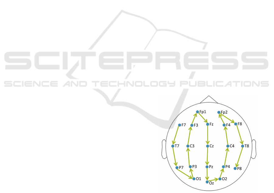
Figure 1: The 20 common channels were used in this study.

The channels ordering process initiates from the left tempo-

ral lobe (starting from F7) and extends to the right temporal

lobe (ending to P8). This deliberate sequence was designed

to formulate 3D inputs as a stack of 2D segments incorpo-

rating inter-channel correlations.

BIOSIGNALS 2024 - 17th International Conference on Bio-inspired Systems and Signal Processing

584

2.2 EEG Signal Pre-Processing

Several ﬁltering procedures were applied to enhance

signal quality. Speciﬁcally, a 125 Hz low-pass ﬁl-

ter and a 1 Hz high-pass ﬁlter were applied to retain

high-frequency signals relevant to abnormal brain ac-

tivities before seizures, while simultaneously remov-

ing DC offset and baseline ﬂuctuations (Allen et al.,

1992; Arroyo and Uematsu, 1992). Moreover, to mit-

igate power line interference, two notch ﬁlters operat-

ing at 50 Hz and 100 Hz were incorporated in the pre-

processing pipeline (Niknazar et al., 2015; Thangavel

et al., 2021). EEG signals were ﬁnally downsampled

to 128 Hz, and the time series were normalized by

subtracting the average EEG reference computed on

each patient’s training data. All ﬁltering operations

were performed using the MNE package within the

Python 3.8.5 version.

2.3 Scalogram Images

The input matrices for CNN models were created by

transforming the EEG time series into scalogram im-

ages, as proposed in recent studies (Yildiz et al., 2021;

Varlı and Yılmaz, 2023). To this aim, the Contin-

uous Wavelet Transform (CWT) was used to com-

pute multiple expansions and the wavelet’s time off-

set, yielding a variety of frequency values for ana-

lyzing continuous-time signals that can be used to

characterize energy density at a local time-frequency

within the transformation (Peng et al., 2002). A more

precise and ﬂexible time–frequency resolution can

be obtained by considering the absolute value of the

CWT when producing scalogram images (Bostanov,

2004), which is particularly effective since it effec-

tively captures high- and low-frequency information

also in non-stationary signals like EEG (Falamarzi

et al., 2014).

More precisely, a function known as the main

wavelet performs the window’s role within the

wavelet transform; during the conversion process, this

main wavelet function is scaled and shifted, enabling

extensive time interval windowing for low frequen-

cies and compressed time interval windowing for high

frequencies (T

urk and

Ozerdem, 2019). The Mor-

let wavelet was employed for the continuous wavelet

transformations (Kareem and Kijewski, 2002). CWT

can be represented mathematically in continuous time

as in Equation (1), where W(s, τ), x(t), (t), s, and τ

represent the wavelet coefﬁcients, the time signal, the

basic wavelet function conjugate, the scale, and the

position parameter, respectively:

(s,τ) =

√

+∞

−∞

x(t)ψ

∗

(

t −τ

)dt (1)

In our study, scalogram images were created us-

ing sliding windows of 30 seconds with 50% over-

lap, resulting in greater accuracy compared to shorter

windows of 10 or 20 seconds. To improve computa-

tional efﬁciency during model training, the resulting

time-frequency scalogram images were resized to 96

× 96 pixels using cubic interpolation, following the

methodology adopted by (Ozdemir et al., 2021) and

urk and

Ozerdem, 2019). Samples of resized scalo-

grams depicting distinct preictal and interictal states

are shown in Fig. 2.

2.4 Deep Learning Architectures

All models were implemented using the PyTorch

framework (version 1.13.0). Training and testing

phases were carried out using a virtual machine

equipped with an Nvidia V100 GPU allocated in the

Google Cloud Platform.

2.4.1 Hyperparameters Tuning

Model hyperparameters were iteratively reﬁned using

a hierarchical strategy to attain the optimal conﬁgu-

ration using a reasonable amount of computing time.

For the LSTM model we tuned the hyperparameters

using the Optuna framework (Akiba et al., 2019); the

search space included the number of hidden layers (1,

2, 3), the size of hidden layers (32, 64, 128, 256),

learning rate (1e-5 to 0.1), batch size (16, 32, 64, 128,

256), and the dropout rates (0.1 to 0.9). The CNNs

hyperparameters were tuned in a speciﬁc order, start-

ing from the number of hidden layers (2, 3, 4), the

number of kernels (16, 32, 64), the kernel size (2, 3,

5), the learning rate (0.01, 0.001, 0.0001), the num-

ber of dropout layers (1, 2, 3), the dropout rate (0.1,

0.2, 0.5), batch size (16, 32, 64) and the use of pool-

ing layers to reduce the size of feature maps progres-

sively. The hyperparameters yielding the best perfor-

mance at each step were selected before progressing

to the next optimization step.

2.4.2 LSTM

The LSTM network received an input time series of 5-

second raw signals with a 3-second overlap, resulting

in an input size of 20 channels × 640 time points. The

ﬁnal LSTM architecture was made up of two hidden

layers, with 32 units each. Two drop-out layers with

a drop-out rate of 0.1 and 0.3 were included between

the two LSTM layers and before the fully connected

layer, respectively. The ﬁnal LSTM architecture is

represented in Fig. 3.

A Comparison of Recurrent and Convolutional Deep Learning Architectures for EEG Seizure Forecasting

585

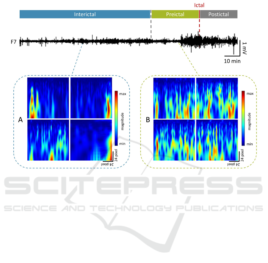
Figure 2: Example of a 145 min EEG signal trace recorded from channel F7 during a seizure event, segmented to identify

interictal vs. preictal states. Panel A shows four different sample images from the interictal state, while panel B shows four

different sample images from the preictal state.

2.4.3 2D CNN

For the 2D convolutional network, scalogram images

originating from each channel were treated indepen-

dently. Consequently, the input dimension for the

2D model was 96 × 96. The ﬁnal architecture com-

prised three convolutional layers, with 16, 32, and 64

kernels, activated by Rectiﬁed Linear Unit (ReLU)

functions and complemented with batch normaliza-

tion layers. The optimal kernel size was 3 × 3 for

all layers, and a stride of 3 and padding of one pixel

was applied. To mitigate the risk of overﬁtting, two

dropout layers with a dropout rate of 0.1 were placed

after the third convolutional layer and the ﬂatting

layer. The ﬂattened layer was further processed by

an additional ReLU-activated dense layer comprising

128 units, and this layer was ﬁnally decoded by an

output layer that used a sigmoid activation function to

produce the model’s prediction.

2.4.4 3D CNN

To create the 3D input, a speciﬁc order of channels

from the left to the right temporal lobe was adopted:

F7, T7, P7, O1, P3, C3, F3, Fp1, Fz, Cz, Pz, Oz, O2,

P4, C4, F4, Fp2, F8, T8, and P8 (see Fig. 1). The

corresponding scalogram images were given as input

to the 3D model, resulting in a 20 × 96 × 96 input

shape. To allow for a fair comparison, the existing

2D CNN optimal architecture was subject to adapta-

tion solely in terms of kernel dimensions, transition-

ing from 2D to 3D. The ﬁnal 3D architecture is repre-

sented in Fig. 4.

2.5 Model Evaluation

All models were trained for 100 epochs, and the train-

ing accuracy was recorded after each epoch in order

to track learning progress over time. Furthermore,

randomized cross-validation was carried out in each

fold by dividing the 93 seizures into 80% train and

20% test sets. However, during the ﬁve-fold cross-

validation implementation, the average accuracy of

testing data points after each fold was considered

to select the best model and compare three models.

Models’ performances were measured using 5-fold

cross-validation in terms of accuracy (ACC), sensi-

tivity (SEN), and speciﬁcity (SPE), which were com-

puted from true positives (TP), false positives (FP),

true negatives (TN), and false negatives (FN) as fol-

lows:

BIOSIGNALS 2024 - 17th International Conference on Bio-inspired Systems and Signal Processing

586

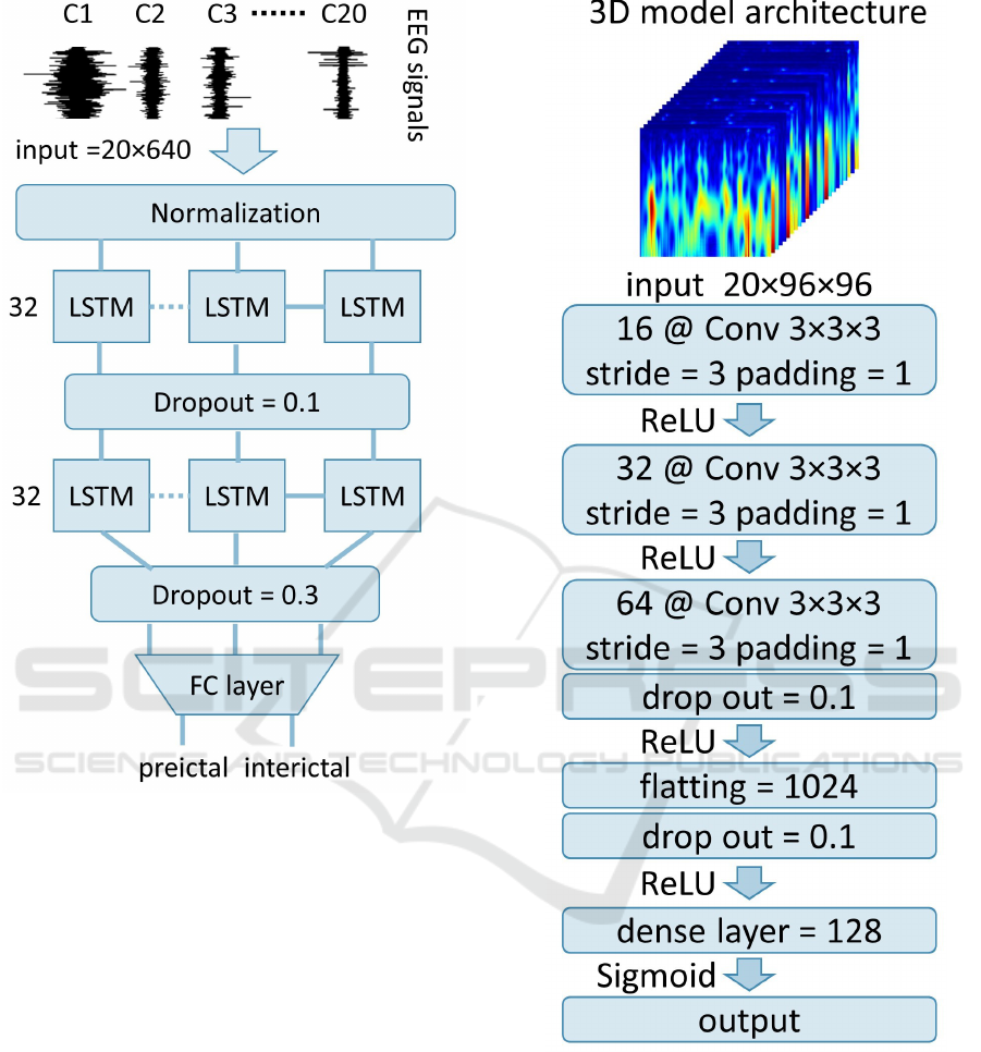
Figure 3: Representation of the ﬁnal LSTM model architec-

ture. The model comprises two LSTM layers with 32 units

each and two drop-out layers with 0.1 and 0.3 rates, respec-

tively.

Accuracy = ((t p + tn)/(t p +tn + f n + f p)) (2)

Sensitivity = (t p/(t p + f n)) (3)

Speci f icity = (tn/(tn + f p)) (4)

In order to evaluate the performance gain of deep

learning models compared to traditional machine

learning classiﬁers, the best-performing architectures

were further benchmarked against an XGBoost clas-

siﬁer trained on a set of 53 EEG features (for details,

see (Shaﬁezadeh et al., 2023)).

Figure 4: Representation of the ﬁnal 3D CNN model ar-

chitecture. The model comprises three convolutional layers

and two drop-out layers. The 2D CNN architecture is iden-

tical, with a kernel dimension of 3 × 3.

3 RESULTS

As shown in Figure 5, the LSTM model converged

to higher accuracy in a smaller number of training

epochs. The ﬁnal performance of the 2D model was

signiﬁcantly lower than the LSTM and 3D models,

suggesting that inter-channel correlations constitute

A Comparison of Recurrent and Convolutional Deep Learning Architectures for EEG Seizure Forecasting

587

Figure 5: Improvement of training accuracy during the ﬁt-

ting of the three deep learning models (3D, LSTM, and 2D).

an important source of information that can be lever-

aged for the seizure prediction task.

In the testing phase, the LSTM model achieved the

highest speciﬁcity at 99.01%, while the 3D model ex-

hibited the highest accuracy and sensitivity, with val-

ues of 98.95% and 98.91%, respectively. ACC, SEN,

and SPE average values of each model in the testing

set, as well as standard deviations of each testing set’s

performance metric after implementation of ﬁve-fold,

are presented in Table 1. This table also illustrates the

results of statistical comparisons (one-way ANOVA)

between the three models after tuning and their best

results. The ﬁndings show signiﬁcant differences be-

tween all performance metrics, and post-hoc Tukey

tests conﬁrmed that the 2D architecture performed

worse than the LSTM and the 3D architectures (see

Table 2).

The LSTM model demonstrated signiﬁcant im-

provements in performance metrics compared to the

2D model, with differences of 9.49%, 7.62%, and

12.46% in ACC, SEN, and SPE, respectively. Also,

the 3D model achieved substantial improvements

compared to the 2D model, respectively of 9.53%,

7.72%, and 11.57%. Although slight variations exist

in the performance metrics between the LSTM and

the 3D model, such differences were not statistically

signiﬁcant. A graphical representation of all perfor-

mance metrics is given in Figure 6.

3.1 Comparison with XGBoost

Having identiﬁed the LSTM and 3D models as the

top-performing models according to all performance

metrics, we then proceeded with a comparison against

a standard machine learning model, speciﬁcally XG-

Boost, trained on a set of 53 ad hoc features extracted

from the EEG signal (for details, see (Shaﬁezadeh

et al., 2023)). The performance metrics of XGBoost

are shown in the gray column of Figure 6.

After applying cross-validation on the fea-

Figure 6: Comparison of the average performance metrics

of the testing set for classifying interictal and preictal phases

with the LSTM, 2D, 3D, and XGBoost models. Error bars

represent the standard deviation of each performance metric

after the implementation of ﬁve-fold cross-validation.

ture data set, the XGBoost model achieved ACC

(75.86%±3.37), SEN (75.90%±5.74), and SPE

(74.72%±4.61). The LSTM model signiﬁcantly out-

performed XGBoost across all evaluation metrics:

23.05% in ACC, 22.91% in SEN, and 24.29% in SPE

(all p-values <0.01). The same results were found for

the 3D model, which signiﬁcantly outperformed XG-

Boost with increases of 23.09% in ACC, 23.01% in

SEN, and 23.40% in SPE (all p-values <0.01). It is

also worth noting that deep learning models are asso-

ciated with substantially reducing the standard error

associated with each evaluation metric, suggesting a

more stable classiﬁcation performance.

4 DISCUSSION

In this study, we leveraged raw signals and scalogram

images derived from multichannel EEG recordings of

epileptic patients to conduct a comparative analysis

between the LSTM, 2D, and 3D models in seizure

forecasting. Our investigation revealed that incorpo-

rating inter-channel correlations by feeding all chan-

nels to the LSTM model and the 3D CNN model

yielded a signiﬁcant (almost 10%) improvement in

accuracy, increasing the classiﬁer precision in distin-

guishing between interictal and preictal states.

A direct benchmarking against a more tradi-

tional XGBoost machine learning classiﬁer further

conﬁrmed that deep learning architectures allow to

achieve substantial performance gains across all eval-

uation metrics. At the same time, it should be noted

that our results are not directly comparable with other

recently published ﬁndings, since our analyses were

carried out using a novel clinical dataset recently col-

lected in a local hospital. However, as a qualita-

tive comparison, we might argue that our ﬁndings

BIOSIGNALS 2024 - 17th International Conference on Bio-inspired Systems and Signal Processing

588

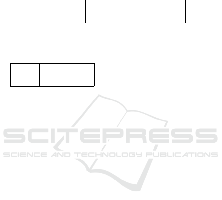
Table 1: Average accuracy (ACC), sensitivity (SEN), and speciﬁcity (SPE) of the testing set obtained by different architectures.

All performance metrics are illustrated by mean(%)±standard deviation after the implementation of ﬁve-fold cross-validation.

The last two columns report the results from the ANOVA.

Metrics LSTM 2D 3D F-value p-value

ACC 98.91±0.34 89.42±1.13 98.95±0.39 234.96 <0.01

SEN 98.81±0.56 91.19±3.79 98.91±0.26 15.97 <0.01

SPE 99.01±0.75 86.55±2.23 98.12±0.73 95.30 <0.01

Table 2: Results of the Tukey post-hoc test to compare per-

formance metrics of the LSTM, 2D, and 3D models. Each

row in the table corresponds to the p-value calculated for

the comparison between two target models in terms of ac-

curacy (ACC), sensitivity (SEN), and speciﬁcity (SPE) of

the testing set.

Models ACC SEN SPE

LSTM - 2D <0.01 <0.05 <0.01

LSTM - 3D 0.996 0.998 0.660

3D - 2D <0.01 <0.01 <0.01

are well-aligned, if not superior, with the accuracy

and sensitivity levels reported in the recent literature:

for example, LSTMs achieved an accuracy of 85.1%

and a sensitivity of 86.8% in a similar seizure predic-

tion task (Varnosfaderani et al., 2021), and 3D CNNs

have been recently shown able to reach an accuracy of

80.50% (Wang et al., 2021) and sensitivity of 85.7%

(Ozcan and Erturk, 2019) in seizure prediction.

5 CONCLUSIONS

While several studies have recently demonstrated that

deep learning models can achieve high accuracy in

seizure prediction tasks by analyzing EEG record-

ings from individual channels, our study suggests that

feeding multiple channels simultaneously, as it hap-

pens in the LSTM and 3D CNN architectures, allows

to exploit inter-channel correlations to improve fore-

casting performance. Furthermore, our results show

that deep learning methods signiﬁcantly outperform

traditional machine learning approaches, supporting

the recent trend of applying neural network models to

the automated analysis of biological signals.

For future work, it would be interesting to investi-

gate channel selection techniques (Jana and Mukher-

jee, 2021) to further establish whether some channels

are more important than others in the seizure predic-

tion task. Especially for focal epilepsy, this would

likely depend on the localization of the seizure source

(e.g., temporal vs. occipital). It would thus be cru-

cial to collect EEG recordings from a larger cohort of

patients in order to make it possible to train source-

speciﬁc models and/or exploit a more heterogeneous

training set to extract generalizable features that can

be used across different patients’ proﬁles. A related

research direction would be to move from random-

ized cross-validation setups to more robust evaluation

schemes, such as those based on leave-one-patient-

out cross-validation (Shaﬁezadeh et al., 2023). How-

ever, this would also require to signiﬁcantly scale-up

the available training datasets, which should allow to

discover more robust predictive features.

Last but not least, it would be important to de-

sign and implement interpretability methods that can

be used to better understand the output produced by

deep learning models. Indeed, in medical settings it

is of paramount importance to deploy explainable AI

methods to improve the reliability of automatic deci-

sion systems (Gunning et al., 2019).

REFERENCES

Abbasi, B. and Goldenholz, D. M. (2019). Machine learn-

ing applications in epilepsy. Epilepsia, 60(10):2037–

2047.

Akiba, T., Sano, S., Yanase, T., Ohta, T., and Koyama, M.

(2019). Optuna: A next-generation hyperparameter

optimization framework. In Proceedings of the 25rd

ACM SIGKDD International Conference on Knowl-

edge Discovery and Data Mining.

Allen, P., Fish, D., and Smith, S. (1992). Very high-

frequency rhythmic activity during EEG suppression

in frontal lobe epilepsy. Electroencephalography and

clinical neurophysiology, 82(2):155–159.

Arroyo, S. and Uematsu, S. (1992). High-frequency EEG

activity at the start of seizures. Journal of Clinical

Neurophysiology, 9(3):441–448.

Assi, E. B., Nguyen, D. K., Rihana, S., and Sawan, M.

(2017). Towards accurate prediction of epileptic

seizures: A review. Biomedical Signal Processing and

Control, 34:144–157.

Bostanov, V. (2004). Bci competition 2003-data sets ib and

iib: feature extraction from event-related brain poten-

tials with the continuous wavelet transform and the t-

value scalogram. IEEE Transactions on Biomedical

engineering, 51(6):1057–1061.

Calesella, F., Testolin, A., De Filippo De Grazia, M., and

Zorzi, M. (2021). A comparison of feature extraction

methods for prediction of neuropsychological scores

from functional connectivity data of stroke patients.

Brain Informatics, 8(1):1–13.

A Comparison of Recurrent and Convolutional Deep Learning Architectures for EEG Seizure Forecasting

589

Falamarzi, Y., Palizdan, N., Huang, Y. F., and Lee, T. S.

(2014). Estimating evapotranspiration from tempera-

ture and wind speed data using artiﬁcial and wavelet

neural networks (wnns). Agricultural Water Manage-

ment, 140:26–36.

Gunning, D., Steﬁk, M., Choi, J., Miller, T., Stumpf, S.,

and Yang, G.-Z. (2019). Xai—explainable artiﬁcial

intelligence. Science robotics, 4(37):eaay7120.

Hochreiter, S. and Schmidhuber, J. (1997). Long short-term

memory. Neural computation, 9(8):1735–1780.

Hussein, R., Lee, S., Ward, R., and McKeown, M. J.

(2021). Semi-dilated convolutional neural networks

for epileptic seizure prediction. Neural Networks,

139:212–222.

Jana, R. and Mukherjee, I. (2021). Deep learning based ef-

ﬁcient epileptic seizure prediction with EEG channel

optimization. Biomedical Signal Processing and Con-

trol, 68:102767.

Ji, S., Xu, W., Yang, M., and Yu, K. (2012). 3d convolu-

tional neural networks for human action recognition.

IEEE transactions on pattern analysis and machine

intelligence, 35(1):221–231.

Kareem, A. and Kijewski, T. (2002). Time-frequency anal-

ysis of wind effects on structures. Journal of Wind

Engineering and Industrial Aerodynamics, 90(12-

15):1435–1452.

LeCun, Y., Bengio, Y., et al. (1995). Convolutional net-

works for images, speech, and time series. The

handbook of brain theory and neural networks,

3361(10):1995.

Liu, Y., Jain, A., Eng, C., Way, D. H., Lee, K., Bui, P.,

Kanada, K., de Oliveira Marinho, G., Gallegos, J.,

Gabriele, S., et al. (2020). A deep learning system

for differential diagnosis of skin diseases. Nature

medicine, 26(6):900–908.

Niknazar, H., Maghooli, K., and Nasrabadi, A. M. (2015).

Epileptic seizure prediction using statistical behavior

of local extrema and fuzzy logic system. international

journal of computer applications, 113(2).

Ozcan, A. R. and Erturk, S. (2019). Seizure prediction

in scalp EEG using 3d convolutional neural networks

with an image-based approach. IEEE Transactions

on Neural Systems and Rehabilitation Engineering,

27(11):2284–2293.

Ozdemir, M. A., Cura, O. K., and Akan, A. (2021). Epilep-

tic EEG classiﬁcation by using time-frequency images

for deep learning. International journal of neural sys-

tems, 31(08):2150026.

Peng, Z., Chu, F., and He, Y. (2002). Vibration signal

analysis and feature extraction based on reassigned

wavelet scalogram. Journal of Sound and Vibration,

253(5):1087–1100.

San-Segundo, R., Gil-Martin, M., D’Haro-Enr

ıquez, L. F.,

and Pardo, J. M. (2019). Classiﬁcation of epileptic

EEG recordings using signal transforms and convo-

lutional neural networks. Computers in biology and

medicine, 109:148–158.

Shaﬁezadeh, S., Duma, G. M., Mento, G., Danieli, A., An-

toniazzi, L., Del Popolo Cristaldi, F., Bonanni, P., and

Testolin, A. (2023). Methodological issues in evaluat-

ing machine learning models for EEG seizure predic-

tion: Good cross-validation accuracy does not guaran-

tee generalization to new patients. Applied Sciences,

13(7):4262.

Thangavel, P., Thomas, J., Peh, W. Y., Jing, J., Yuvaraj, R.,

Cash, S. S., Chaudhari, R., Karia, S., Rathakrishnan,

R., Saini, V., et al. (2021). Time–frequency decompo-

sition of scalp electroencephalograms improves deep

learning-based epilepsy diagnosis. International jour-

nal of neural systems, 31(08):2150032.

Tsiouris, K. M., Pezoulas, V. C., Zervakis, M., Konitsio-

tis, S., Koutsouris, D. D., and Fotiadis, D. I. (2018).

A long short-term memory deep learning network for

the prediction of epileptic seizures using EEG signals.

Computers in biology and medicine, 99:24–37.

urk,

O. and

Ozerdem, M. S. (2019). Epilepsy detection by

using scalogram based convolutional neural network

from EEG signals. Brain sciences, 9(5):115.

Usman, S. M., Khalid, S., and Aslam, M. H. (2020). Epilep-

tic seizures prediction using deep learning techniques.

Ieee Access, 8:39998–40007.

Van Mierlo, P., Vorderw

ulbecke, B. J., Staljanssens,

W., Seeck, M., and Vulli

emoz, S. (2020). Ictal

EEG source localization in focal epilepsy: Review

and future perspectives. Clinical Neurophysiology,

131(11):2600–2616.

Varlı, M. and Yılmaz, H. (2023). Multiple classiﬁcation

of EEG signals and epileptic seizure diagnosis with

combined deep learning. Journal of Computational

Science, 67:101943.

Varnosfaderani, S. M., Rahman, R., Sarhan, N. J.,

Kuhlmann, L., Asano, E., Luat, A., and Alhawari,

M. (2021). A two-layer lstm deep learning model for

epileptic seizure prediction. In 2021 IEEE 3rd Inter-

national Conference on Artiﬁcial Intelligence Circuits

and Systems (AICAS), pages 1–4. IEEE.

Wang, Z., Yang, J., and Sawan, M. (2021). A novel multi-

scale dilated 3d cnn for epileptic seizure prediction.

pages 1–4.

World Health Organization (2023). Epilepsy, https://www.

who.int/en/news-room/fact-sheets/detail/epilepsy.

Yildiz, A., Zan, H., and Said, S. (2021). Classiﬁcation and

analysis of epileptic EEG recordings using convolu-

tional neural network and class activation mapping.

Biomedical signal processing and control, 68:102720.

BIOSIGNALS 2024 - 17th International Conference on Bio-inspired Systems and Signal Processing

590