Solving Job Shop Problems with Neural Monte Carlo Tree Search

Marco Kemmerling

, Anas Abdelrazeq

and Robert H. Schmitt

Chair of Production Metrology and Quality Management & Institute for Information Management in Mechanical

Engineering (WZL-MQ/IMA), RWTH Aachen University, Aachen, Germany

Keywords:

Neural Monte Carlo Tree Search, Reinforcement Learning, AlphaZero, Job Shop Problem, Combinatorial

Optimization.

Abstract:

Job shop scheduling is a common NP-hard problem that ﬁnds many applications in manufacturing and beyond.

A variety of methods to solve job shop problems exist to address different requirements arising from individual

use cases. Recently, model-free reinforcement learning is increasingly receiving attention as a method to train

agents capable of scheduling. In contrast, model-based reinforcement learning is less well studied in job

scheduling. However, it may be able to improve upon its model-free counterpart by dynamically spending

additional planning budget to reﬁne solutions according to the available scheduling time at any given moment.

Neural Monte Carlo tree search, a family of model-based algorithms including AlphaZero is especially suitable

for discrete problems such as the job shop problem. Our aim is to ﬁnd suitable designs of neural Monte

Carlo tree search agents for the job shop problem by systematically varying certain parameters and design

components. We ﬁnd that different choices for the evaluation phase of the tree search have the biggest impact

on performance and conclude that agents with a combination of node value initialization using learned value

functions and roll-out based evaluation lead to the most favorable performance.

1 INTRODUCTION

The job shop problem (JSP), like many other combi-

natorial optimization problems, is NP-hard, meaning

that no polynomial-time algorithms capable of com-

puting exact solutions are known. In practice, it is of-

ten preferable to apply efﬁcient algorithms that ﬁnd

reasonably good solutions, rather than spend large

amounts of computational budget to compute exact

optima.

In recent times, reinforcement learning has been

receiving increasing attention as a method to train

agents capable of solving JSPs (Zhang et al., 2020;

Samsonov et al., 2021). While some variation in

agent design and modeling of the problem exist, in

many cases, reinforcement learning is used to essen-

tially learn scheduling heuristics. While this requires

considerable training time, agents can compute solu-

tions at low computational cost after training and have

been demonstrated to outperform common schedul-

ing heuristics such as shortest processing time ﬁrst

(SPT) and longest processing time ﬁrst (LPT) (Sam-

https://orcid.org/0000-0003-0141-2050

https://orcid.org/0000-0002-8450-2889

https://orcid.org/0000-0002-0011-5962

sonov et al., 2021). A further potential beneﬁt of re-

inforcement learning approaches is the ability to learn

tailor-made heuristics that exploit the characteristics

of speciﬁc use cases.

While exact methods are often not suitable in dy-

namic use cases with quickly changing circumstances

due to their high computational cost, the low compu-

tational cost of trained reinforcement learning agents

forms another extreme and may leave much untapped

potential. In practice, the available decision time bud-

get may not be sufﬁcient for exact methods, but there

often is non-negligible budget to be used, which may

vary from decision to decision (McKay and Wiers,

2003; Govind et al., 2008). It may hence be de-

sirable to spend this additional computational bud-

get to further improve solution quality. While this is

not possible using typical model-free reinforcement

learning approaches, model-based approaches such as

neural Monte Carlo Tree Search (MCTS) (Kemmer-

ling et al., 2024) allow for dynamic adjustments of

the computational budget to accommodate use case

and situation-speciﬁc requirements. At the same time,

neural MCTS retains the ability of model-free ap-

proaches to learn to exploit problem characteristics.

Neural MCTS algorithms gained attention when

AlphaGo marked a paradigm shift in computational

Kemmerling, M., Abdelrazeq, A. and Schmitt, R.

Solving Job Shop Problems with Neural Monte Carlo Tree Search.

DOI: 10.5220/0012311700003636

Paper published under CC license (CC BY-NC-ND 4.0)

In Proceedings of the 16th International Conference on Agents and Artiﬁcial Intelligence (ICAART 2024) - Volume 3, pages 149-158

ISBN: 978-989-758-680-4; ISSN: 2184-433X

149

approaches to combinatorial games by beating a hu-

man champion in the game of Go (Silver et al., 2016),

followed by the successes of AlphaGo Zero (Silver

et al., 2017) and AlphaZero (Silver et al., 2018).

While the success of neural MCTS algorithms in

combinatorial games has been clearly established, it is

less clear how well such approaches transfer to prob-

lems outside of games, such as the JSP and combina-

torial optimization problems in general. To facilitate

such a transfer, some modiﬁcations to algorithms in

the AlphaZero family have to be made, since the char-

acteristics of games differ from the characteristics of

other problems in many ways, e.g. in their notion of

multiple players. Even those design choices in Alp-

haZero that can be directly transferred to the JSP may

not be the most beneﬁcial in terms of performance

for this new problem. It is hence not clear what the

exact design of neural MCTS approaches for the JSP

should be. Indeed, neural MCTS approaches to prac-

tical problems feature a wide range of different design

choices (Kemmerling et al., 2024). The limited num-

ber of publications on this topic typically present a

ﬁnished solution, i.e. one speciﬁc design of a neural

MCTS algorithm without comparisons against alter-

native designs. We believe that a systematic investi-

gation of the effects of different design choices will be

valuable to practitioners trying to ascertain the right

design for their respective applications. To take a step

towards this vision, we perform such a systematic in-

vestigation for the JSP, as one representative of com-

binatorial optimization problems.

In the remainder of this work, we ﬁrst give some

background on neural MCTS in Section 2 and de-

scribe the current research landscape on neural MCTS

for scheduling in Section 3. In Section 4, we model

the problem and describe our experimental setup, fol-

lowed by the results stemming from this setup in Sec-

tion 5, and a conclusion in Section 6.

2 NEURAL MONTE CARLO

TREE SEARCH

MCTS is a heuristic search method developed for

combinatorial game playing. To ﬁnd appropriate

moves, it constructs a search tree based on random

sampling, in which nodes correspond to states and

edges to actions. Although MCTS developed inde-

pendently from reinforcement learning, the two ex-

hibit many similarities including the formulation of

policies and the estimation of state values. For a more

in depth discussion on this connection, the reader is

referred to Vodopivec et al. (2017). MCTS produces

policies π

MCT S

and value estimates v

MCT S

for speciﬁc

states, while modern reinforcement learning typically

aims to produce policies and value functions that gen-

eralize across states.

In the following, we focus on the single-player

version of MCTS, which assumes state transitions to

only be dependent on the current state and the selected

action, but not the actions of a further independent

player.

MCTS iteratively constructs its search tree by re-

peatedly performing a series of four phases start-

ing from the root of the tree: (1) selection, (2) ex-

pansion, (3) evaluation, (4) back-propagation, all of

which may vary slightly from one implementation to

another. Generally, in the selection phase, the next ex-

isting tree node to be visited is selected by choosing

an action for the current node’s state. This selection is

performed by balancing exploration of less explored

tree branches and exploitation of known high-value

branches, usually in the form of some version of a

Upper Conﬁdence Bound for Trees (UCT) formula:

a = argmax

W (s, a)

N(s,a)

+ c

ln N(s)

N(s,a)

(1)

where W (s,a) is the cumulative reward of each

time action a has been chosen in state s, N(s,a) in-

dicates how often a has been chosen in s, N(s) are the

total visits of s and c is a constant weighting the explo-

ration term. The left part of the sum encourages ex-

ploitation while the right part encourages actions that

have been performed seldomly in the current state.

Once a leaf node is encountered in the selection

phase, the expansion phase begins and adds a subset

or all possible children to the current leaf node. At

this point, it is unclear what the value of these children

should be. To estimate the value of each newly ex-

panded node, standard MCTS procedure is to perform

random roll-outs from the node’s corresponding state

until a terminal state is reached and a reward is re-

ceived. This reward then forms the initial value of the

node and is propagated up the tree in the last MCTS

phase to update the value of all nodes preceding the

newly expanded ones. In a variant of this procedure,

not the newly expanded nodes, but the leaf node pre-

ceding them is evaluated. This reduces the number of

evaluations in each MCTS search but requires some

other way of initializing the newly expanded nodes’

values.

The MCTS procedure described above can be

modiﬁed to incorporate guidance by neural networks

in the ﬁrst three phases. While this can take many dif-

ferent shapes, we evaluate only a subset of the varia-

tions surveyed during our previous review (Kemmer-

ling et al., 2024). In the selection phase, next to the

standard UCT rule described above, we also consider

ICAART 2024 - 16th International Conference on Agents and Artiﬁcial Intelligence

150

the AlphaZero variant of the Predictor + UCT (PUCT)

rule (Silver et al., 2018):

a = argmax

W (s, a)

N(s,a)

+ c P(s,a)

N(s)

1 + N(s,a)

(2)

which introduces a prior probability P(s,a) pro-

duced by a policy neural network to further weight

the exploration term.

In the expansion phase, we consider full expan-

sion and a type of neural expansion which expands

only a subset of all possible children. This subset is

constructed as the smallest subset of potential chil-

dren whose policy probabilities sum to a given thresh-

old τ. Finally, in the evaluation phase, we consider

two possible neurally guided options next to random

roll-outs: roll-outs according to the learned policy,

and estimating a node’s value directly by the learned

function.

The neural guidance networks can then be trained

by a procedure called policy improvement by MCTS,

which alternatingly performs two steps: performing

a neural MCTS search guided by the current state of

the neural networks and subsequently using the re-

sults from the search π

MCT S

(s) and V

MCT S

(s) as train-

ing targets for the neural networks. Alternatively, the

neural networks can be trained by conventional means

such as supervised or model-free reinforcement learn-

ing and then simply used to guide MCTS at decision

time.

More information about neural MCTS can be

found in our previous literature review (Kemmerling

et al., 2024). For reference, AlphaZero is a neural

MCTS algorithm that consists of selection based on

the PUCT rule, full expansion, evaluation by a learned

value function and trains the underlying neural net-

work solely using policy improvement by MCTS (Sil-

ver et al., 2018).

3 RELATED WORK

Neural MCTS has received relatively little attention

in the context of the JSP. Rinciog et al. (2020) train

a neural MCTS agent to solve a special case of the

JSP in sheet metal scheduling, while G

oppert et al.

(2021) model a dynamically interconnected assembly

system as a ﬂexible job shop problem and train a neu-

ral MCTS agent to solve it. Both approaches orient

themselves closely on the AlphaZero architecture, in

which the MCTS phases take the form of PUCT selec-

tion, full expansion, and evaluation by a learned value

function. In both cases, neural networks are trained

by supervised learning on targets from a scheduling

heuristic. While Rinciog et al. (2020) additionally

train using policy improvement by MCTS after the

supervised training phase, the additional training only

leads to a marginally improved performance com-

pared to the employed scheduling heuristic.

Next to this small amount of research focused

on JSPs, neural MCTS has also been investigated

for further, related scheduling problems. These in-

clude parallel machine scheduling problems (Wang

et al., 2020; Oren et al., 2021) as well as directed

acyclic graph task scheduling (Cheng et al., 2019; Hu

et al., 2019). The exact approaches of these individ-

ual works vary. Some use learned policy roll-outs for

the evaluation phase instead of learned value function

evaluations (Wang et al., 2020; Cheng et al., 2019; Hu

et al., 2019), some use standard tree policies in the se-

lection phase (Oren et al., 2021; Hu et al., 2019), and

some employ neural expansion (Cheng et al., 2019;

Hu et al., 2019). To train the agents, PPO (Wang et al.,

2020), Q-Learning (Oren et al., 2021) and a combi-

nation of supervised pre-training and policy gradient

methods (Cheng et al., 2019; Hu et al., 2019) are used,

while training using policy improvement by MCTS is

not reported in any of the approaches.

The existing literature on neural MCTS in

scheduling problems hence features a considerable

amount of variation, but contains few comparisons of

different algorithmic variants under identical experi-

mental settings. A previously performed survey on

neural MCTS applications beyond scheduling (Kem-

merling et al., 2024) shows that neural MCTS ap-

proaches in general can be even more varied than the

currently existing approaches in scheduling. In the

face of this diversity in approaches, it is unclear which

kind of algorithmic conﬁguration is appropriate for a

given problem such as the JSP and what the advan-

tages and disadvantages of particular design choices

in the conﬁguration of neural MCTS agents are. This

points to a need for studies systematically assessing

the effect of different design choices, which we aim

to provide for the JSP in this document.

4 METHODS

4.1 Markov Decision Process

To train neural MCTS agents, we create an environ-

ment by modelling the JSP as a Markov decision pro-

cess (MDP), and deﬁne a corresponding observation

space, action space, and reward function. While de-

signing these components is crucial to the success of

any employed method, we aim to create a setup that is

functional but otherwise as simple as possible to keep

Solving Job Shop Problems with Neural Monte Carlo Tree Search

151

the focus on our main object of study.

Generally, the agent’s task is to schedule a set of

jobs J , with each job j ∈ J consisting of a set of op-

erations O

∈ O. In our case, the agent constructs a

schedule by iteratively selecting jobs whose ﬁrst un-

scheduled operation is then placed at the earliest pos-

sible time of the existing partial schedule.

Observation Space. Our observation space is a

simpliﬁed version of the one proposed by Zhang

et al. (2020), consisting of two vectors: A vector of

length |O| in which every element corresponds to the

scheduling status of one particular operation. If the

operation has been scheduled already, the correspond-

ing element is 1, otherwise it is 0. Operations are

grouped into jobs and ordered by precedence con-

straints. The second vector is similarly structured

such that each element contains a lower bound on the

corresponding operation’s completion time.

Action Space. We employ a discrete action space

with size |J |, where each action a

, i = 0, . ..,|J | cor-

responds to scheduling the next operation o of job j

the earliest possible time. This means that, at the lat-

est, we schedule it on its required machine m just after

the last scheduled operation on m ﬁnishes processing.

However, if there is a large enough gap between two

already scheduled operations on m, we instead sched-

ule o within the identiﬁed gap.

Reward Function. We employ a sparse reward

function that evaluates the terminal state s

cor-

responding to a completed schedule based on its

makespan C

max

, i.e. the time the last operation ﬁn-

ishes processing. Instead of directly using the nega-

tive makespan as a reward, we use the negative op-

timality gap with regard to a pre-computed optimum

opt

, as deﬁned by Equation (3).

r(s

) = −

max

−C

opt

(3)

While the requirement for known optima makes

this reward function unsuitable for practical settings,

in experimental settings such as ours it provides a

clear, unbiased reward signal that is easy to interpret.

4.2 Experimental Setup

All agents in our experiments are trained using the

JSP instances provided by Samsonov et al. (2022),

which are split into training set (90%) and test set

(10%). The experiments in the following section are

initially restricted to instances of size 6 ×6 to al-

low for more thorough experimentation while keep-

ing computational costs manageable. In Section 5.4,

the scaling properties of neural MCTS algorithms are

then investigated on instances of size 15 ×15.

Neural MCTS agents are trained using policy im-

provement by MCTS, which consists of alternatingly

collecting experience using MCTS and subsequent

training of the neural networks on experience sam-

pled from a replay buffer. In each policy improve-

ment iteration, 40 episodes of experience are col-

lected which are then stored in a ﬁrst-in ﬁrst-out re-

play buffer of size 36000. Unless otherwise speciﬁed,

each action is determined by performing 100 MCTS

simulations n

MCT S

, i.e. completing all four MCTS

phases 100 times. During training, one epoch of expe-

rience is sampled from the buffer to train the networks

in batches of size 256 using the Adam optimizer.

The employed neural networks are standard feed-

forward networks with two hidden layers of size 256

and Mish activation functions (Misra, 2019). Policy

and value networks are fully independent.

Next to neural MCTS agents, we train a Proximal

Policy Optimization (PPO) baseline using the stable-

baselines3 package (Rafﬁn et al., 2019). For prob-

lems of size 6×6, we use a learning rate of 5E-05 and

the same network architecture as for the neural MCTS

agents. For problems of size 15 ×15, we use a learn-

ing rate of 1E-05, a clip range of 0.01 and a network

with three hidden layers of size 512 each. All other

hyper-parameters are kept at their default values.

5 RESULTS

To evaluate the effects of the different design choices

outlined in Section 2, we perform a series of experi-

ments using the setup described above. The ﬁrst ex-

periment aims to establish a ﬁrst understanding of the

effects of different factors, while the second aims to

reduce the computational cost associated with each

training run, thereby facilitating a much larger and

thorough third experiment.

Our ﬁrst experiment follows a full factorial de-

sign with the following factors: (1) selection pol-

icy with levels UCT and PUCT, each with c = 1.0,

(2) expansion policy with levels full expansion and

neural expansion with τ = 0.9, (3) evaluation policy

with levels random roll-out, learned policy roll-out,

and learned value function evaluation, and (4) eval-

uated nodes with levels encountered leaf and newly

expanded nodes.

For each combination of these factors, we train a

separate neural MCTS agent and evaluate it on the test

ICAART 2024 - 16th International Conference on Agents and Artiﬁcial Intelligence

152

set. Our response, or evaluation metric, is the average

reward of an agent on all test set instances.

While there is considerable variance in these aver-

age rewards for differently conﬁgured neural MCTS

agents, the best agent achieves an average optimal-

ity gap of 4.3%. We perform an analysis of variance

(ANOVA) of the results (see Table 1) and ﬁnd that

only different choices in evaluation policy and which

nodes are evaluated lead to statistically signiﬁcant dif-

ferences in the rewards of the corresponding agents.

Table 1: ANOVA results of a full factorial experiment with

four factors. Interactions between factors are not consid-

ered. All results matching a signiﬁcance level of < 0.05 are

highlighted in bold.

Factor df SS MS F PR(> F)

Sel. pol. 1 0.00 0.00 0.00 9.51E-01

Exp. pol. 1 0.01 0.01 1.65 2.15E-01

Eval. pol. 2 0.07 0.04 7.12 5.26E-03

Eval. nodes 1 0.33 0.33 64.14 2.41E-07

Residual 18 0.09 0.01

Between these two factors, the choice of which

nodes to evaluate has the biggest impact. The

boxplots in Figure 1 show that the average reward

when only evaluating encountered leaves is between

−0.3 and −0.4 regardless of the evaluation method.

When newly expanded nodes are evaluated instead,

the performance of all evaluation methods increases,

although only a modest improvement can be ob-

served when using learned value evaluation. The

performance of the two roll-out methods undergoes

a more dramatic improvement with average rewards

> −0.05. Surprisingly, random roll-outs appear to

slightly outperform policy-guided roll-outs.

In summary, in this experiment, MCTS agents

with neural guidance do not achieve better results than

MCTS agents without neural guidance and the per-

formance of the agents is clearly dominated by the

number of evaluated nodes. The number of evalu-

ated nodes, however, has a big impact on the com-

putational cost of the algorithms. Especially with

the more expensive evaluation methods based on roll-

outs, evaluating all newly expanded nodes can lead

to undesirably long run times. While evaluating all

expanded nodes using learned value evaluation is a

fairly cheap operation requiring only a single neural

network call, the resulting performance is only mod-

erately better than evaluating only the encountered

leaf.

In the following, we aim to combine the best of

both approaches by initializing each newly expanded

node with a learned value estimate and additionally

evaluating the encountered leaf with a roll-out.

5.1 Initializing Nodes & Trees

We investigate two initialization methods, the ﬁrst

of which works as described above, i.e. by using a

learned value function to initialize node values. While

the value estimates may not be perfect, this type of

initialization is meant to provide the search some

guidance especially early on, when the search space

has not been explored much. The second method ful-

ﬁlls a similar purpose, but operates on the tree level

instead of the node level. Here, we populate the ini-

tial tree by one full roll-out of a learned policy. The

ﬁrst initialization method will be referred to as value

initialization, while the second one will be referred to

as tree initialization in the following.

As depicted in Figure 2, both initialization meth-

ods lead to a signiﬁcant performance improvement

compared to evaluating only encountered leaves with-

out any additional initialization method. On aver-

age, value initialization alone leads to higher rewards

than tree initialization and applying both initialization

methods at the same time, albeit with slightly higher

variance. Comparing these results to the ones in the

previous section, it becomes clear that evaluating only

leaves and applying value initialization can match the

performance of evaluating all expanded nodes, but at

much reduced computational cost.

5.2 Additional Design Choices

The number of design choices in the previous exper-

iments has been very limited both in the factors and

their levels to get a ﬁrst overview of their effects and

arrive at agent conﬁgurations that achieve good re-

sults within reasonable time. In the following, we per-

form a more thorough examination comprising more

factors than before, but we limit ourselves to agents

with value initialization and evaluation of encoun-

tered leaves. We again investigate different choices

for the selection policy, the expansion policy, and

evaluation policy, but consider a much larger num-

ber of levels for each of these factors (see Table 2).

For the selection policy we consider PUCT rules with

a larger variety of exploration constants and for the

expansion policy we consider a larger number of neu-

ral expansion thresholds, where a threshold of τ = 1.0

corresponds to full expansion. Additionally, we vary

the number of MCTS simulations and the weights of

the individual loss components (see Table 2). To ac-

complish the latter while keeping the number of ex-

perimental factors limited, we introduce factors for

Solving Job Shop Problems with Neural Monte Carlo Tree Search

153

Evaluate

Encountered

Leaves

Evaluate

Expanded

Nodes

−0.4

−0.3

−0.2

−0.1

Random

Roll-out

Evaluate

Encountered

Leaves

Evaluate

Expanded

Nodes

Learned Policy

Roll-out

Evaluate

Encountered

Leaves

Evaluate

Expanded

Nodes

Learned Value

Evaluation

Avg. Reward

Figure 1: Effects of the two signiﬁcant factors evaluation policy and evaluated nodes visualized as boxplots of the average

test set reward.

Table 2: Tukey’s honestly signiﬁcant difference (HSD) test on the factors with signiﬁcant results in the preceding ANOVA.

Signiﬁcant differences between the means of two levels are highlighted in bold. Positive values in the mean difference column

indicate that the second group in the row leads to better results.

Factor Group 1 Group 2 Mean Diff. p-Adj. Lower Upper Reject

Entropy

Loss

Weight

0.1 0.33 0.0051 0.6191 -0.0077 0.0179 False

0.1 0.5 0.0076 0.3498 -0.0053 0.0204 False

0.33 0.5 0.0025 0.8944 -0.0104 0.0153 False

Value

Loss

Weight

0.1 0.33 0.0002 0.9994 -0.0127 0.013 False

0.1 0.5 0.0037 0.7776 -0.0091 0.0165 False

0.33 0.5 0.0035 0.7968 -0.0093 0.0164 False

Number

Simulations

10 50 0.0304 0.0 0.0143 0.0464 True

10 100 0.0401 0.0 0.0241 0.0561 True

10 200 0.0469 0.0 0.0309 0.0629 True

50 100 0.0097 0.4024 -0.0063 0.0257 False

50 200 0.0166 0.0396 0.0005 0.0326 True

100 200 0.0068 0.6906 -0.0092 0.0229 False

Selection

Policy

PUCT, c=0.1 PUCT, c=0.5 -0.0022 0.9978 -0.0215 0.017 False

PUCT, c=0.1 PUCT, c=1 -0.0058 0.926 -0.025 0.0135 False

PUCT, c=0.1 PUCT, c=10 -0.016 0.1587 -0.0352 0.0033 False

PUCT, c=0.1 UCT, c=1 -0.001 0.9999 -0.0203 0.0183 False

PUCT, c=0.5 PUCT, c=1 -0.0035 0.9876 -0.0228 0.0158 False

PUCT, c=0.5 PUCT, c=10 -0.0137 0.2956 -0.033 0.0056 False

PUCT, c=0.5 UCT, c=1 0.0012 0.9998 -0.018 0.0205 False

PUCT, c=1 PUCT, c=10 -0.0102 0.5991 -0.0295 0.0091 False

PUCT, c=1 UCT, c=1 0.0048 0.9621 -0.0145 0.024 False

PUCT, c=10 UCT, c=1 0.015 0.2127 -0.0043 0.0342 False

Neural

Expansion

Threshold

1.0 0.5 -0.148 0.0 -0.161 -0.1349 True

1.0 0.8 -0.0563 0.0 -0.0693 -0.0432 True

1.0 0.9 0.0067 0.5535 -0.0064 0.0197 False

0.5 0.8 0.0917 0.0 0.0786 0.1047 True

0.5 0.9 0.1547 0.0 0.1416 0.1677 True

0.8 0.9 0.063 0.0 0.0499 0.076 True

Eval

Policy

Learned Policy Learned Value -0.1463 0.0 -0.1559 -0.1367 True

Learned Policy Random 0.0005 0.9908 -0.0091 0.0101 False

Learned Value Random 0.1468 0.0 0.1372 0.1564 True

the value loss L

and entropy loss L

, but set the pol-

icy loss implicitly as L

= 1 −L

−L

We perform a full factorial experiment on all these

factors with a total of 2160 differently conﬁgured

ICAART 2024 - 16th International Conference on Agents and Artiﬁcial Intelligence

154

Initialisation

Tree

Initialisation

Value

Initialisation

Both

−0.4

−0.3

−0.2

−0.1

Avg. Reward

Figure 2: Effects of different initialization methods on test

set rewards.

agents. To limit the time required to train all these

agents, we reduce the number of policy iterations

from 100 in the previous experiments to 30, as little

improvement could be observed past 30 iterations in

the previous experiments.

An ANOVA of the results of this experiment

shows that signiﬁcant differences exist between the

means of levels of all factors. We select Tukey’s HSD

as a post-hoc test to analyze which design choices are

especially beneﬁcial and display the results in Table 2.

The results are consistent with the previous experi-

ments, with the evaluation policy being the most im-

pactful factor. The choice of exploration constant in

the selection policy does not lead to signiﬁcant dif-

ferences, and larger neural expansion thresholds gen-

erally lead to better results. As expected, the qual-

ity of solutions increases with the number of simu-

lations. A point of diminishing returns appears to be

reached fairly quickly, however, as 200 simulations do

not lead to signiﬁcantly improved results compared to

100 simulations.

Weighting the loss components differently does

not result in signiﬁcantly different outcomes. How-

ever, when examining the average entropy of both

the learned policy vectors and the MCTS policy vec-

tor of an agent, it becomes clear that, not only do

they correlate with each other, there is also a relation-

ship between the entropy and the achieved rewards.

As Figure 3 shows, the highest rewards are achieved

only when the entropy of the learned policy vector is

roughly > 0.75, but not below. Similarly, the highest

rewards are observed when the entropy of the MCTS

policy vector is > 0.5.

While different agent conﬁgurations lead to dif-

ferences in performance, design choices also have an

effect on the computational expense of an agent. This

is mainly reﬂected in the number of times the dynam-

ics model and the neural networks are called, which

is primarily determined by the employed evaluation

method. The exact run time will then depend on hard-

ware and the efﬁciency and complexity of both the dy-

namics model and the neural network. In Figure 3, the

impact of the three different evaluation methods on

model and neural network calls is visualized. While

learned value function evaluation unsurprisingly leads

to the smallest amount of model calls and may there-

fore be especially efﬁcient in many cases, this is un-

likely to be of interest, as the resulting performance

lacks far behind the other two methods. Among these

other two roll-out methods, the number of model calls

is comparable, but the learned policy roll-out method

makes many more neural network calls than the ran-

dom roll-out method. In light of the comparable qual-

ity of their achieved solutions, the random roll-out

method is clearly preferable in practice.

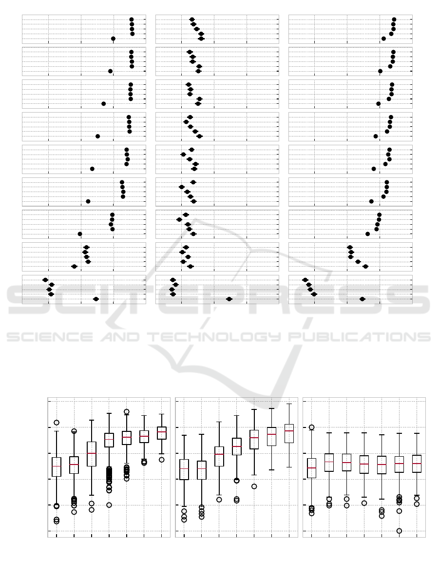
5.3 The Impact of MCTS Budget

One promise of neural MCTS is the ability to vary the

search budget n

MCT S

at decision time to achieve the

best possible solutions given current time constraints.

Each of the n

MCT S

search iterations consists of com-

pleting the four MCTS phases. In the following, we

investigate the effect of different search budgets, both

during training and at decision time.

As Figure 4 shows, the search budget at deci-

sion time has a strong inﬂuence on solution quality,

with larger budgets generally leading to better solu-

tions. This is the case for all evaluation methods, al-

though the improvement is less pronounced when us-

ing learned value function evaluation. Surprisingly,

the search budget during training has only a small ef-

fect on solution quality. When using random eval-

uation, the effect of different n

MCT S

during training

is negligible, while learned policy evaluation beneﬁts

from larger search budgets during training to a small

degree. This trend is reversed on very small decision

time budgets (n

MCT S

< 10), presumably because the

policy network learns to maximize rewards given only

few look-ahead searches.

When the policies trained using policy improve-

ment by MCTS are used model-free, i.e. without any

decision-time search, they are generally inferior to

policies trained by PPO. For any decision time bud-

get n

MCT S

≥ 10, employing a policy trained by PPO

in the tree search leads to signiﬁcantly worse results,

with the exception of agents with learned value func-

tion evaluation.

The best agent conﬁgurations with n

MCT S

= 200

and n

MCT S

= 100, achieve average test set rewards of

−0.041 and −0.046, respectively. For comparison,

the average SPT, LPT and PPO rewards are −0.161,

−0.217, −0.167, respectively.

Solving Job Shop Problems with Neural Monte Carlo Tree Search

155

0.2 0.4 0.6 0.8

MCTS Entropy

0.2

0.3

0.4

0.5

0.6

0.7

0.8

0.9

Learned Policy Entropy

0.0 0.5 1.0 1.5 2.0

Neural Net Calls ×10

0.0

0.5

1.0

1.5

2.0

2.5

3.0

Model Calls ×10

Learned Policy

Random

Learned Value

−0.400

−0.375

−0.350

−0.325

−0.300

−0.275

−0.250

−0.225

−0.200

Reward

Figure 3: Left: Each agent’s average policy distribution entropy as computed by the learned policy and by MCTS. Right:

Total calls to the model and to the neural networks over the course of the training.

5.4 Scaling to Larger Instances

The previous experiments are concerned with rela-

tively small instances of size 6 ×6. To investigate

the scaling properties of neural MCTS on larger in-

stances, we train differently conﬁgured agents on

15 ×15 instances in a full factorial experiment. In

this case, the factors are comprised of the selection

policy, the expansion policy, and the evaluation pol-

icy. The selection policy can either be a UCT or

PUCT rule, each with c = 1.0 and the expansion pol-

icy can either be full expansion or neural expansion

with τ = 0.9. Since training 15 ×15 instances is gen-

erally more computationally expensive and the pre-

vious experiments show that the MCTS budget dur-

ing training does not have a big impact, we set it to a

lower value of n

MCT S

= 10.

As shown in Figure 5, the impact of different

evaluation policies follows a similar pattern as on

the smaller instances. Evaluation by a learned value

function leads to signiﬁcantly worse results than the

two roll-out based methods. Compared to the previ-

ous experiments, random roll-outs and learned policy

roll-outs switch places with the neurally guided roll-

outs performing better on average, especially when

MCT S

≤ 10. This reversal may indicate that neural

guidance provides a useful bias in exploring the in-

creased search space of larger instances, whereas in

smaller instances, unbiased evaluation methods are

preferable as the search space can be more easily cov-

ered. The best performing agent achieves an aver-

age test set reward of −0.179 compared to −0.269,

−0.377, and −0.335 for SPT, LPT and PPO.

6 CONCLUSION

We set out to gain an understanding of the effect of

different neural MCTS design choices and to arrive

at agent conﬁgurations with strong performance on

the JSP. While many forms of neural guidance do not

have a clear beneﬁt in our experiments, agents with a

combination of node value initialization and roll-out

based evaluation signiﬁcantly outperform a model-

free baseline trained by PPO at reasonable computa-

tional cost. Further, we ﬁnd that the MCTS search

budget used during training has only a minor effect

on the trained agent’s performance, while the search

budget during decision time is much more inﬂuential.

This means that agents can be trained relatively efﬁ-

ciently with small budgets and that the budget at deci-

sion time can be varied dynamically to adhere to sit-

uational time constraints while maximizing decision

quality.

Our investigation is concerned with a subset of

all possible design choices of neural MCTS agents,

but further experiments with additional factors may

reveal agents with even more favorable properties.

These may include mixed evaluation policies with

different mechanisms depending on the depth of the

node to be evaluated, mechanisms that exploit max-

imum node values instead of average ones, reward

functions based on self-competition, and many more.

One illuminating future research direction may be

in investigating what kinds of scheduling situations

call for neural MCTS and what situations are ade-

quately addressed by model-free approaches.

ICAART 2024 - 16th International Conference on Agents and Artiﬁcial Intelligence

156

1000

Random Learned Value

100

200

Learned Policy

500

100

200

100

200

100

200

100

200

100

200

100

200

100

200

-0.30 -0.20 -0.10 0.00

-0.30 -0.20 -0.10 0.00 -0.30 -0.20 -0.10 0.00

100

200

Training MCTS Budget

Decision Time MCTS Budget

Avg. Test Set Reward

Training MCTS Budget

Decision Time MCTS Budget

Training MCTS Budget

Decision Time MCTS Budget

Figure 4: The effect of the search budget n

MCT S

at decision time (rows) and during training (vertical axis in each subplot) on

the average reward on the test set (horizontal axes). Results are divided into the three different evaluation methods: random

roll-outs (left), learned value function evaluation (middle), and learned policy roll-outs (right). A training budget n

MCT S

= 0

corresponds to an agent trained by PPO, and a decision time budget n

MCT S

= 0 corresponds to the trained policy being applied

in a model-free manner, without any search at decision-time.

0 1 5 10 25 50 100

−1.0

−0.8

−0.6

−0.4

−0.2

0.0

Learned Policy

0 1 5 10 25 50 100

Random

0 1 5 10 25 50 100

Learned Value

Decision Time MCTS Budget

Avg. Test Reward

Figure 5: Test set performance of neural MCTS agents with different evaluation policies on 15 ×15 instances. The MCTS

budget at decision time is varied, but held constant at n

MCT S

= 10 during training.

Solving Job Shop Problems with Neural Monte Carlo Tree Search

157

ACKNOWLEDGEMENTS

Funded by the Deutsche Forschungsgemeinschaft

(DFG, German Research Foundation) under Ger-

many’s Excellence Strategy – EXC-2023 Internet of

Production – 390621612.

ROLES & CONTRIBUTIONS

Marco Kemmerling: Conceptualization, Methodol-

ogy, Software, Visualization, Writing – Original Draft

Anas Abdelrazeq: Writing - Review & Editing

Robert H. Schmitt: Project administration, Funding

REFERENCES

Cheng, Y., Wu, Z., Liu, K., Wu, Q., and Wang, Y. (2019).

Smart DAG tasks scheduling between trusted and un-

trusted entities using the MCTS method. Sustainabil-

ity, 11(7):1826. Publisher: MDPI.

Govind, N., Bullock, E. W., He, L., Iyer, B., Krishna, M.,

and Lockwood, C. S. (2008). Operations management

in automated semiconductor manufacturing with inte-

grated targeting, near real-time scheduling, and dis-

patching. IEEE Transactions on Semiconductor Man-

ufacturing, 21(3):363–370. Publisher: IEEE.

oppert, A., Mohring, L., and Schmitt, R. H. (2021).

Predicting performance indicators with ANNs for

AI-based online scheduling in dynamically intercon-

nected assembly systems. Production Engineering,

15(5):619–633. Publisher: Springer.

Hu, Z., Tu, J., and Li, B. (2019). Spear: Optimized

Dependency-Aware Task Scheduling with Deep Re-

inforcement Learning. In 2019 IEEE 39th Interna-

tional Conference on Distributed Computing Systems

(ICDCS), pages 2037–2046.

Kemmerling, M., L

utticke, D., and Schmitt, R. H. (2024).

Beyond Games: A Systematic Review of Neural

Monte Carlo Tree Search Applications. Applied In-

telligence. Publisher: Springer (In Press).

McKay, K. N. and Wiers, V. C. (2003). Planning, schedul-

ing and dispatching tasks in production control. Cog-

nition, Technology & Work, 5:82–93. Publisher:

Springer.

Misra, D. (2019). Mish: A self regularized non-monotonic

activation function. arXiv preprint arXiv:1908.08681.

Oren, J., Ross, C., Lefarov, M., Richter, F., Taitler, A.,

Feldman, Z., Di Castro, D., and Daniel, C. (2021).

SOLO: search online, learn ofﬂine for combinatorial

optimization problems. In Proceedings of the Inter-

national Symposium on Combinatorial Search, vol-

ume 12, pages 97–105. Issue: 1.

Rafﬁn, A., Hill, A., Ernestus, M., Gleave, A., Kanervisto,

A., and Dormann, N. (2019). Stable baselines3.

Rinciog, A., Mieth, C., Scheikl, P. M., and Meyer, A.

(2020). Sheet-metal production scheduling using Al-

phaGo Zero. In Proceedings of the Conference on

Production Systems and Logistics: CPSL 2020.

Samsonov, V., Hicham, K. B., and Meisen, T. (2022). Rein-

forcement Learning in Manufacturing Control: Base-

lines, challenges and ways forward. Engineering Ap-

plications of Artiﬁcial Intelligence, 112. Publisher:

Elsevier.

Samsonov, V., Kemmerling, M., Paegert, M., L

utticke, D.,

Sauermann, F., G

utzlaff, A., Schuh, G., and Meisen,

T. (2021). Manufacturing Control in Job Shop En-

vironments with Reinforcement Learning. In Pro-

ceedings of the International Conference on Agents

and Artiﬁcial Intelligence: ICAART 2021, volume 2,

pages 589–597.

Silver, D., Huang, A., Maddison, C. J., Guez, A., Sifre, L.,

Van Den Driessche, G., Schrittwieser, J., Antonoglou,

I., Panneershelvam, V., Lanctot, M., and others

(2016). Mastering the game of Go with deep neural

networks and tree search. nature, 529(7587):484–489.

Publisher: Nature Publishing Group.

Silver, D., Hubert, T., Schrittwieser, J., Antonoglou, I., Lai,

M., Guez, A., Lanctot, M., Sifre, L., Kumaran, D.,

Graepel, T., and others (2018). A general reinforce-

ment learning algorithm that masters chess, shogi, and

Go through self-play. Science, 362(6419):1140–1144.

Publisher: American Association for the Advance-

ment of Science.

Silver, D., Schrittwieser, J., Simonyan, K., Antonoglou,

I., Huang, A., Guez, A., Hubert, T., Baker, L.,

Lai, M., Bolton, A., and others (2017). Mastering

the game of go without human knowledge. nature,

550(7676):354–359. Publisher: Nature Publishing

Group.

Vodopivec, T., Samothrakis, S., and Ster, B. (2017). On

monte carlo tree search and reinforcement learning.

Journal of Artiﬁcial Intelligence Research, 60:881–

936.

Wang, J. H., Luo, P. C., Xiong, H. Q., Zhang, B. W.,

and Peng, J. Y. (2020). Parallel Machine Workshop

Scheduling Using the Integration of Proximal Policy

Optimization Training and Monte Carlo Tree Search.

In 2020 Chinese Automation Congress (CAC), pages

3277–3282. IEEE.

Zhang, C., Song, W., Cao, Z., Zhang, J., Tan, P. S., and Xu,

C. (2020). Learning to dispatch for job shop schedul-

ing via deep reinforcement learning. arXiv preprint

arXiv:2010.12367.

ICAART 2024 - 16th International Conference on Agents and Artiﬁcial Intelligence

158