Benchmarking a Wide Range of Unsupervised Learning Methods for

Detecting Anomaly in Blast Furnace

Kendai Itakura

, Dukka Bahadur

and Hiroto Saigo

School of Information Science and Electrical Engineering, Kyushu University, Fukuoka, Japan

Department of Computer Science, Michigan Technological University, Houghton, U.S.A.

Keywords:

Anomaly Detection, Time Series, Steel Production, Deep Learning, Unsupervised Learning.

Abstract:

Steel plays important roles in our daily lives, as it surrounds us in the form of various products. Blast furnace,

one of the main facility in steel production process, is traditionally monitored by skilled workers to prevent

incidents. However, there is a growing demand to automate the monitoring process by leveraging machine

learning. This paper focuses on investigating the suitability of unsupervised learning methods for detecting

anomalies in blast furnaces. Extensive benchmarking is conducted using a dataset collected from blast fur-

naces, encompassing a wide range of unsupervised learning methods, including both traditional approaches

and recent deep learning-based techniques. The computational experiments yield results that suggest the ef-

fectiveness of traditional methods over deep learning-based methods. To validate this observation, additional

experiments are performed on publicly available non time series datasets and complex time series datasets.

These experiments serve to conﬁrm the superiority of traditional methods in handling non time series datasets,

while deep learning methods exhibit better performance in dealing with complex time series datasets. We

have also discovered that dimensionality reduction before anomaly detection is beneﬁcial in eliminating out-

liers and effectively modeling the normal data points in the blast furnace dataset.

1 INTRODUCTION

Steel plays important roles in our daily lives, as it

surrounds us in the form of various products such as

automobiles, electrical appliances, bridges, pipes and

railroad. The production facility of steel requires sig-

niﬁcant investment, making it proﬁtable to improve

production efﬁciency. A key component of the facil-

ity is blast furnace, which is used for extracting iron

and other metals. Since any accidents in blast furnace

can lead to substantial production loss or delays, pre-

venting such incidents by anomaly detection is neces-

sary.

Anomaly detection in blast furnace is tradition-

ally done manually by skilled workers who analyze

the data obtained through pressure sensors. However,

the level of expertise can vary among individuals,

highlighting the need for an automated process. This

paper explores the applicability of machine learning

methods for detecting anomalies in blast furnaces and

evaluates their performance using a collected dataset.

The dataset are obtained from the pressure sensors

equally arranged inside the blast furnace at certain

time intervals. The resulting data can be stored in a

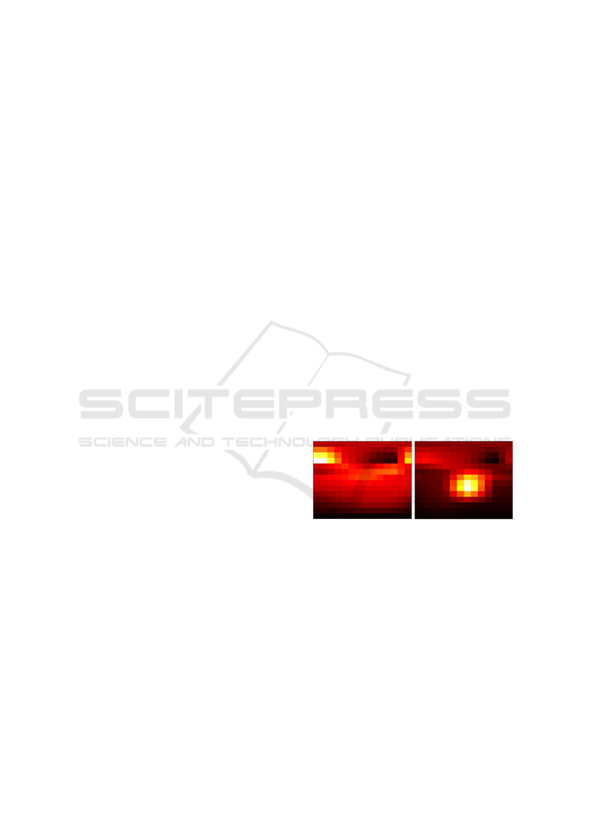
Figure 1: The blast furnace has 196 evenly distributed sen-

sors that provide pressure readings at regular intervals. An

anomaly is deﬁned as a large pressure deviation, which is

simply labeled as normal or not by calculating the variance.

Normal (left) and anomalous (right) data point consist of 16

× 16 measurements.

sequence of matrices, or a tensor. Figure 1 displays

examples of normal data and anomalous data mea-

sured at a speciﬁc time point, respectively.

Due to the nature of the dataset, anomalies are rare

compared to normal data. Furthermore, manually an-

notation is hard if we consider the size of the dataset.

These facts motivates us to make use of unsupervised

learning, with which we do not need to model anoma-

lousness, but only need to model normality. As a re-

sult, the anomalies can be detected by the deviations

Itakura, K., Bahadur, D. and Saigo, H.

Benchmarking a Wide Range of Unsupervised Learning Methods for Detecting Anomaly in Blast Furnace.

DOI: 10.5220/0012310800003654

Paper published under CC license (CC BY-NC-ND 4.0)

In Proceedings of the 13th International Conference on Pattern Recognition Applications and Methods (ICPRAM 2024), pages 641-650

ISBN: 978-989-758-684-2; ISSN: 2184-4313

641

Figure 2: Categorization of anomaly detection models.

from normality. In general, anomaly is considered as

an observation that deviates signiﬁcantly from some

normal concept. Anomaly detection or outlier de-

tection, is the research area that studies the detection

of such anomalous observations through methods and

models. In this paper we examine various anomaly

detection algorithms, ranging from traditional ones to

recent ones. To get an overview, we introduce the

categorization, originally introduced in (Ruff et al.,

2021). Figure 2 summarized the anomaly detection

methods used in this paper, and their categorization.

We compared various anomaly detection methods

in terms of detection performance in the blast furnace

dataset, where we found that traditional methods per-

formed better than recent ones based on deep learn-

ing. In order to conﬁrm this observation, we have

also run the same methods on two types of bench-

mark datasets, that is, non-time series datasets and

complex time series datasets, where we have corrob-

orated that the traditional methods performs better in

non-time series datasets, while the deep methods per-

formed better in complex time series datasets. We

have also found that dimensionality reduction could

boost the performance of most of the methods when

we have sufﬁciently large training dataset. Our con-

tributions are as follows:

1. Extensive benchmarking of anomaly detection

methods both in the blast furnace dataset and pub-

lic benchmark datasets.

2. Empirically understanding the types of data that

each method excels at and struggles with.

3. Effectiveness of dimensionality reduction when a

training dataset includes both normal and anoma-

lous data points.

The rest of the paper is organized as follows. In Sec-

tion 2, we review anomaly detection methods by their

categories. Section 3 describes the experimental set-

tings and discusses the obtained results. Section 5

concludes the paper with discussion.

2 ANOMALY DETECTION

METHODS

In this section, we review anomaly detection methods

based on the categories given in Figure 2. The method

described in Figure 2 is explained below.

2.1 Classiﬁcation Models

Binary classiﬁcation is an elementary problem in

supervised learning settings, and the correspon-

dent in unsupervised settings are one-class clas-

siﬁcation models. Examples include One Class

SVM (OCSVM) (Sch

olkopf and Smola, 2002) and

Support Vector Data Description (SVDD) (Tax and

Duin, 2004). As their names imply, they have the

same spirit as SVM (Huang and LeCun, 2006) for

binary classiﬁcation, and aim at directly ﬁnding the

separating hyperplane that discriminates normal data

from anomalous data, instead of estimating distri-

bution of normal data. Both of them can handle

non-linearity through the use of non-linear kernels.

DSVDD (Ruff et al., 2018) is deep learning version of

SVDD. GOAD (Bergman and Hoshen, 2020) is self-

supervised learning that uses afﬁne transformations

of the data as labels. ICL (Shenkar and Wolf, 2021)

learns mappings that maximize the mutual informa-

tion between each sample and the part to be masked

in order to capture the structure of the samples in a

single training class. Likewise, NeuTraL (Qiu et al.,

2021) uses self-supervised learning to detect anoma-

lies.

2.2 Probabilistic Models

Probabilistic models are those involve estimating the

probability distribution of normal data. The degree

of anomaly of a test data point is measured by the

distance from the normal data distribution. Classi-

cal density estimation methods such as Kernel Den-

sity Estimators (KDE) (Latecki et al., 2007) or his-

tograms (Goldstein and Dengel, 2012) are therefore

examples of probabilistic models. Gaussian Mix-

ture Model (GMM) (Aggarwal et al., 2015) also es-

timates distributions by maximizing the sample pos-

terior probabilities. ECOD (Li et al., 2022) estimates

the distribution of input data by computing an em-

pirical cumulative distribution for each dimension of

data. COPOD (Li et al., 2020) constructs an empir-

ical copula and predicts the tail probability for each

given data set. SOD (Kriegel et al., 2009) takes the

deviation in the subspace along the axis as the degree

of anomaly.

ICPRAM 2024 - 13th International Conference on Pattern Recognition Applications and Methods

642

Figure 3: A schematic ﬁgure that illustrates reconstruction

models. In the training phase, the encoder and decoder are

trained to reconstruct the training data, speciﬁcally focus-

ing on learning the low-dimensional representation Z of the

training data. In the test phase, anomalous data that was not

encountered during the training phase cannot be effectively

reconstructed, leading to a signiﬁcant discrepancy between

the input and its corresponding reconstruction. This dis-

crepancy is referred to as the reconstruction error, which

serves as a measure of anomaly.

2.3 Reconstruction Models

Models based on reconstruction are most common

and have long history. In this model, normal data are

assumed to be correctly reconstructed, and anoma-

lous data are those fail to reconstruct. Principal Com-

ponent Analysis (PCA) (Shyu et al., 2003) is one

of the earliest method. Kernel PCA (KPCA) (Hoff-

mann, 2007) is a kernelized version of PCA, and can

detect anomaly in non-linear space through the us-

age of non-linear kernels. Autoencoders (AE) (Ag-

garwal et al., 2015) uses deep learning for encoding

and decoding of data, and considered as a deep learn-

ing version of PCA. Variational Autoencoder (VAE)

(Kingma and Welling, 2013) is a probabilistic ver-

sion of AE. Generative Adversarial Networks (GAN)

(Goodfellow et al., 2014), like VAE, is a well-known

generative model, consisting of a generator and a dis-

criminator. The generator learns to map from latent

space to data space, and the discriminator learns to

distinguish between real data and samples generated

by the GAN. Adversarially Learned Anomaly Detec-

tion (ALAD) (Zenati et al., 2018) evaluates how far

away the sample is from the reconstruction by the

GAN. RCA (Liu et al., 2021a) obtained robustness by

training multiple autoencoders and discarding sam-

ples with large reconstruction errors. RDP (Wang

et al., 2019) trains a neural network to predict data

distances in a randomly projected space. Prototype

methods such as k-means (Hartigan and Wong, 1979)

can also be considered as reconstruction model, since

reconstruction errors are calculated by the distance

from data points to nearest prototypes, similarly to

PCA.

2.4 Distance Models

If we can assume that the data points in high-density

regions to be normal and the data points in low-

density regions to be anomalous, then the distance

based models are available. For example, Local Out-

lier Factor (LOF) (Breunig et al., 2000) is a method

for estimating density, CBLOF (He et al., 2003) com-

bines LOF with clustering, COF (Tang et al., 2002)

assigns a degree of outlier to each data. Feature bag-

ging (FB) (Lazarevic and Kumar, 2005) is trained

on various subsamples of the data with LOF to sup-

press overﬁtting and increase prediction accuracy.

A simple and popular approach, K-nearest neigh-

bor (KNN)(Ramaswamy et al., 2000) can also be used

for anomaly detection by considering data points far

from the neighbors as anomalous. Isolation-based

Anomaly Detection Using Nearest-Neighbor Ensem-

bles (INNE) (Bandaragoda et al., 2018) divides the

data space into regions using subsamples, determines

an isolation score for each region, and uses the near-

est neighbor ensemble. This detects both global and

local anomalies. Figure 4 displays a schematic ﬁg-

ure that illustrates the way how distance models can

be used for anomaly detection. The Isolation For-

est method (Liu et al., 2008) uses the characteristic

that the number of data splits increases in a high-

density region. REPEN (Pang et al., 2018) learns low-

dimensional representations of ultrahigh-dimensional

data for distance-based outlier detectors.

2.5 Transformer Models

Transformer (Vaswani et al., 2017) is a model that

can handle sequential information such as sentence

and time series. Unlike RNN and LSTM, it does

not have recursion and learns time series by posi-

tion encodings. Reformer (Kitaev et al., 2020) and

Informer (Zhou et al., 2021) have reduced Trans-

former’s drawbacks such as high computation and

memory usage, while Autoformer (Wu et al., 2021)

proposed an Auto-Correlation mechanism instead of

a self-attention mechanism. FEDformer (Zhou et al.,

2022) used Fourier and wavelet transforms to perform

the attention operations in the frequency domain.

Pyraformer (Liu et al., 2021b) realized O(N) com-

plexity by using pyramidal attention modules (N is

the input time series length). Crossformer (Zhang and

Yan, 2022) has a hierarchical encoder-decoder that

captures not only temporal dependence but also inter-

variable dependence. Timesnet (Wu et al., 2022), on

the other hand, uses the Fast Fourier Transform (FFT)

to transform a one-dimensional time series into a two-

dimensional one, thereby capturing complex depen-

Benchmarking a Wide Range of Unsupervised Learning Methods for Detecting Anomaly in Blast Furnace

643

Figure 4: A schematic ﬁgure that illustrates distance mod-

els. In the training phase, the normal data are clustered. In

the test phase, the distance between each test data point and

the center of its nearest cluster is calculated, then the dis-

tance is used as the measure of abnormality.

dencies more effectively.

3 EXPERIMENTS

3.1 Dataset

3.1.1 Blast Furnace Dataset

The ﬁrst dataset we use is collected from blast fur-

nace, and we use 5000 data points as test set. Each

data point corresponds to a 16 × 16 pressure mea-

surement taken every minute. We prepared three dif-

ferent training datasets, and named them as BF1, BF2

and BF3, respectively. BF1 contains no anomalous

data, and only consists of 2000 normal data points.

BF2 contains 7 anomalous data points, and 1993 nor-

mal data points. BF3 contains 39 anomalous data

points, and 19961 normal data points. The relation-

ship among each training dataset and test dataset is

illustrated in Figure 5.

3.1.2 External Benchmark Datasets

In order to ensure that we have correctly conducted

experiments, we have run the same approaches in two

kinds of datasets. One is a non-time series dataset

introduced in (Campos et al., 2016). The 16 multi-

variate datasets utilized in this study are listed in Ta-

ble 2. AR in the table represents the Anomaly Ratio

(%). Since these datasets contain a mixture of anoma-

lous and normal data, we randomly selected 50% of

the normal data and used as a training set, following

the experimental settings in literature (Bergman and

Hoshen, 2020). The test set consists of the remaining

normal data and all anomalous data.

The another dataset is a collection of ﬁve time

series datasets shown in Table 3. MSL and SMAP

(Hundman et al., 2018) represent data obtained from

ISA (Incident Surprise, Anomaly) reports provided by

NASA’s Mars Curiosity (MSL) and Soil Moisture Ac-

tive Passive (SMAP) satellite. PSM (Pooled Server

Figure 5: Training / test split of the blast furnace dataset.

Metrics) (Abdulaal et al., 2021) is collected from mul-

tiple application server nodes at eBay. SMD (Server

Machine Dataset) (Su et al., 2019) is a dataset ob-

tained from the server machine with metrics such

as CPU load, network usage, memory usage, etc.

SWaT (Secure Water Treatment) (Mathur and Tippen-

hauer, 2016) is obtained from sensors of the infras-

tructure system.

3.2 Anomaly Detection Software

The anomaly detection and outlier detection libraries

we used are PyOD (Python Outlier Detection) (Zhao

et al., 2019), DeepOD (Xu et al., 2023), TSlib (Time

Series Library) (Wu et al., 2022), Scikit-learn (Pe-

dregosa et al., 2011). Basically, the implementation

in the library is used with default parameters. How-

ever, some parameters, such as the dimensions of the

hidden layer of the autoencoder, are set manually.

3.3 Settings for Transformer Models

In order to make use of the ability of Transformer

models to handle time series inputs, we concatenate

the training data points without allowing overlapping.

In the blast furnace data, the window size was set to

10. It results in the decrease in the number of avail-

able training data points to 1/10 th, in comparison

to non-time series anomaly detection methods. The

window size for the public time series data was set to

100.

3.4 Effect of Dimensionality Reduction

We also investigated the effect of dimensionality re-

duction to anomaly detection performance. In this

experiments, six dimensionality reduction methods

(PCA, KPCA, AE, VAE, t-SNE (Van der Maaten

ICPRAM 2024 - 13th International Conference on Pattern Recognition Applications and Methods

644

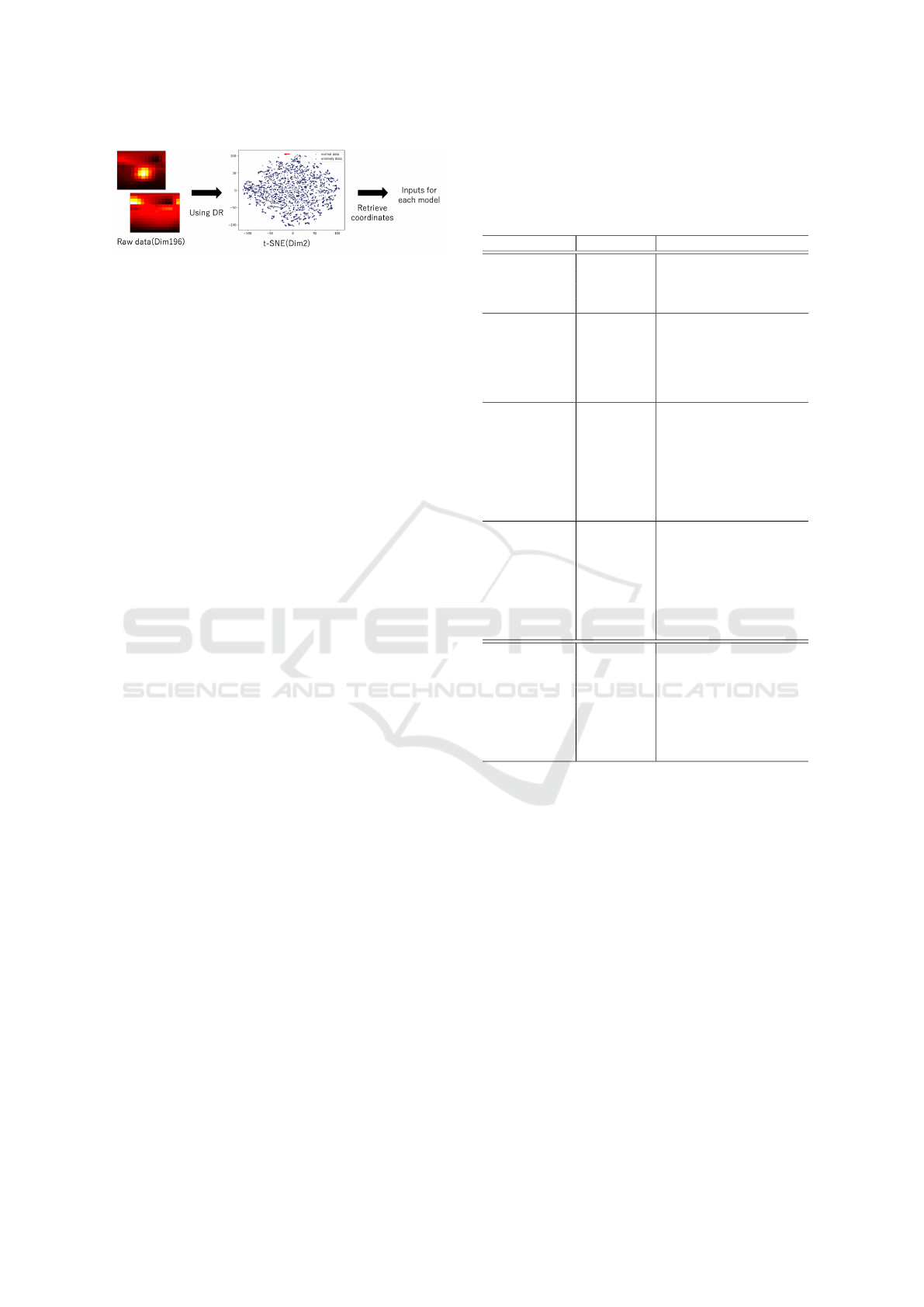
Figure 6: Using dimensionality reduction for anomaly de-

tection.

and Hinton, 2008), and UMAP (McInnes et al.,

2018)) are compared, and the anomaly detection per-

formance in combination with unsupervised learning

methods are investigated. Figure 6 illustrates the pro-

cedure of this experiments.

Both t-distributed Stochastic Neighbor Embed-

ding (t-SNE) and Uniform Manifold Approximation

and Projection (UMAP) have been developed for di-

mensionality reduction for visualization purposes. t-

SNE consists of a two-step algorithm. First, a prob-

ability distribution is constructed in such a way that

data point pairs with high similarity are selected,

while the data points with low similarity are unlikely

to be selected. Next, it deﬁnes a similar probability

distribution on a low-dimensional map and ﬁnds the

location of the point in the low-dimensional map that

minimizes the amount of Kullback-Leibler informa-

tion between the two distributions.

UMAP is based primarily on manifold theory and

topological data analysis. UMAP uses local mani-

fold approximations and their local fuzzy simplical

set representations are stitched together to construct a

topological representation of high-dimensional data.

Given a low-dimensional representation of the data,

a similar process can be used to construct an equiv-

alent topological representation. UMAP then opti-

mizes the layout of the data representation in the low-

dimensional space to minimize the cross-entropy be-

tween the two topological representations.

The dimensionality of PCA and KPCA after di-

mension reduction is set to 12. AE and VAE con-

sist of four hidden layers, where each layer having

dimensions of [128, 63, 32, 16]. The dimensionality

of t-SNE is set to 2, while that of UMAP set to 15.

3.5 Evaluation Metrics

In general, the data used for anomaly detection con-

sists mostly of normal data, with a small amount

of anomalous data. Therefore, if all the test data

were predicted as normal, it would result in an unex-

pectedly high accuracy. To address this, we employ

Precision-Recall Area Under the Curve (PRAUC),

since it can ignore the effect of the large number of

true negatives. PRAUC takes values between 0 and 1,

Table 1: Anomaly detection performance in the blast fur-

nace datasets in terms of PRAUC. For models with † in the

model name, the average of 10 trials is reported because the

results vary from trial to trial. The best score in each dataset

is highlighted in bold fonts.

Type Model BF1 BF2 BF3

Classiﬁcation

DSVDD .326 .145 .350

ICL .00766 .136 .529

NeuTral .0230 .0126 .00862

GOAD .774 .634 .186

Probabilistic

KDE .930 .529 .253

GMM .654 .633 .865

ECOD .0173 .0162 .0196

COPOD .0285 .0212 .0209

HBOS .0142 .00850 .0157

SOD .0512 .0472 .0500

Reconstruction

kmeans† .486 .00488 .456

PCA .174 .151 .137

KPCA .853 .528 .667

AE .175 .153 .137

VAE .230 .198 .138

ALAD† .0121 .00637 .00733

RCA .593 .622 .543

RDP .462 .138 .801

Distance

KNN .773 .345 .666

LOF .715 .228 .253

CBLOF .291 .299 .328

COF .0215 .0279 .0112

IF† .0266 .0134 .0320

FB† .739 .278 .185

INNE† .508 .434 .723

REPEN .358 .603 .501

Timeseries

Transformer .556 .561 .609

Autoformer .388 .388 .448

Crossformer .568 .563 .579

FEDformer .387 .388 .456

Informer .557 .564 .608

Pyraformer .575 .576 .613

Reformer .550 .558 .607

Timesnet .162 .160 .280

with higher values closer to 1 indicating better perfor-

mance.

4 RESULTS

4.1 Training Without Anomalous

Samples

Column BF1 in Table 1 displays the results of

anomaly detection, where anomalous samples are not

used during training. Among the methods evaluated,

KDE achieved the highest score (.930), followed by

KPCA (.853). Several methods that utilize the dis-

tance from training data as an anomaly measure, such

as KNN, LOF, and FB, also turned out to be effec-

tive. Autoencoder-based methods (AE, VAE, RCA)

performed reasonably well, while GAN-based meth-

Benchmarking a Wide Range of Unsupervised Learning Methods for Detecting Anomaly in Blast Furnace

645

Table 2: Statistics of non time series datasets.

Train Test(ano) AR Dim

Arrhythmia 122 328(206) 62.8 259

Cardio 827 1299(471) 36.3 21

HeartDisease 75 195(120) 61.5 13

Hepatitis 33 47(13) 27.7 19

InternetAds 1405 1859(454) 24.4 1555

Ionosphere 112 239(126) 52.7 32

KDDCup99 30193 30439(246) .808 41

Lymphography 71 77(6) 7.79 19

Pima 250 518(268) 51.7 8

Shuttle 500 513(13) 2.53 9

SpamBase 1394 3207(1813) 56.5 57

Stamps 154 186(31) 16.7 9

Waveform 1671 1772(100) 5.64 21

WBC 222 232(10) 4.31 9

WDBC 178 189(10) 5.29 30

WPBC 75 123(47) 38.2 33

ods (ALAD) failed. Transformer models that incor-

porate time series data exhibited fair performance.

4.2 Training with Anomalous Samples

Column BF2 in Table 1 presents the results anomaly

detection when training dataset includes anomalous

samples. In comparison to training without anoma-

lous samples, the performance of many models de-

creased from that of BF1. However, models that in-

corporate time series, such as the Transformer mod-

els, exhibit less performance degradation, suggesting

their robustness in handling anomalous data. Among

the models evaluated, GOAD achieved the highest

score of .634.

4.3 Large Scale Training with

Anomalous Samples

Column BF3 in Table 1 displays the results of

anomaly detection when training is done with large

datasets including anomalous samples. The highest

score of .865 was achieved by GMM. There was no

clear overall trend in performance compared to those

from BF2, suggesting a small impact of the data set

size on the anomaly detection performance. On the

other hand, all the transformer models have shown

a clear trend that the performance increases with re-

spect to the increase in the dataset size.

4.4 Benchmarking with Public Datasets

4.4.1 Non Time Series Data Sets

The anomaly detection performance of various unsu-

pervised methods are shown in Table 4. KPCA per-

Table 3: Statistics of time series datasets.

Training Test AR Dim Length

MSL 58317 73729 .105 55 100

PSM 132481 87841 .278 25 100

SMAP 135183 427617 .121 51 100

SMD 708405 708420 .042 38 100

SWaT 495000 449919 .018 51 100

formed best, followed by KNN and KDE. We can ver-

ify that methods that performed good in blast furnace

datasets also performed good in these benchmark

datasets. Ionosphere dataset has the highest rank cor-

relation coefﬁcient (.748) with the blast furnace data,

suggesting the similarity of the two datasets.

4.4.2 Time Series Datasets

The anomaly detection performance of various meth-

ods in time series datasets are presented in Table 5.

Due to the large data size of the time series dataset, we

could not run all the methods due to memory problem

or time restriction. Traditional models such as KDE,

KNN and KPCA were not effective in terms of both

feasibility and performance. In contrast, models that

take into account the time series property, such as the

Transformer models, obtained excellent scores in the

entire time series dataset. It suggests the necessity of

large number of data points for training Transformer

models.

4.5 Effect of Dimensionality Reduction

on Anomaly Detection Performance

Table 6 shows the anomaly detection performance

after dimensionality reduction in the blast furnace

dataset BF3. Due to the space restriction, we omit the

results for the BF1 and BF2 dataset, but only sum-

marizes the statistics in Table 7. Underlined cells in

the table highlight the improvement of performance

in terms of mean AUC or mean ranks. We can ob-

serve that 30 out of 34 models gained performance

improvement after dimensionality reduction. The per-

formance improvements were notable with PCA and

KPCA in the transformer models, and with UMAP

in the rest of the models. We can also observe in

Table 7 that the performance gain was obtained with

BF1 and BF2 as well, suggesting the effectiveness of

dimensionality reduction in general, in the blast fur-

nace dataset.

ICPRAM 2024 - 13th International Conference on Pattern Recognition Applications and Methods

646

Table 4: Anomaly detection performance of various unsupervised methods in non time series datasets in terms of PRAUC.

Type Model BF1 Arr Car Heart Hapa Inter Ion KDD Lym Pima Shu Spam Stamp Wave WBC WDBC WPBC Mean(Rank)

Classiﬁcation

DSVDD .33 .84 .52 .85 .45 .70 .95 .27 .87 .55 .087 .75 .25 .12 .52 .50 .38 .538(22)

ICL .0077 .75 .36 .81 .32 .61 .93 .74 .72 .62 .59 .82 .31 .11 .17 .55 .37 .549(21)

NeuTral .023 .77 .45 .77 .30 .74 .96 .28 .35 .55 .70 .77 .19 .41 .12 .053 .41 .489(23)

GOAD .77 .71 .41 .57 .21 .50 .98 .55 .42 .49 .71 .54 .15 .048 .045 .43 .40 .448(24)

Probabilistic

KDE .93 .85 .70 .89 .57 .80 .98 .54 1.0 .74 .71 .88 .61 .24 .76 .71 .36 .709(3)

GMM .65 .86 .67 .89 .69 .80 .98 .58 .77 .70 .55 .84 .55 .07 .85 .66 .35 .676(8)

ECOD .017 .85 .66 .68 .49 .61 .78 .46 .91 .64 .074 .67 .41 .079 .93 .63 .32 .575(20)

COPOD .029 .86 .54 .77 .61 .61 .8 .47 .91 .70 .094 .69 .49 .11 .93 .81 .36 .610(17)

HBOS .014 .86 .56 .89 .67 .28 .63 .31 .94 .74 .11 .82 .56 .096 .82 .76 .35 .587(18)

SOD .051 .82 .38 .68 .34 .38 .92 .11 .3 .61 .12 .64 .26 .084 .55 .3 .36 .428(26)

Reconstruction

kmeans† .49 .88 .69 .86 .52 .60 .96 .54 1.0 .72 .67 .85 .58 .19 .68 .77 .34 .678(7)

PCA .17 .88 .73 .86 .71 .59 .92 .53 1.0 .70 .32 .84 .54 .093 .88 .71 .34 .665(11)

KPCA .85 .88 .70 .88 .59 .79 .98 .73 1.0 .72 .70 .87 .58 .22 .75 .72 .36 .717(1)

AE .18 .88 .77 .84 .69 .59 .93 .53 1.0 .67 .31 .84 .54 .093 .89 .66 .32 .660(12)

VAE .23 .88 .73 .86 .71 .59 .93 .53 1.0 .70 .32 .84 .54 .093 .89 .72 .33 .666(10)

ALAD† .012 .71 .47 .72 .27 .38 .67 .025 .059 .52 .034 .67 .34 .052 .17 .27 .51 .367(27)

RCA .59 .88 .69 .87 .67 .60 .98 .53 1.0 .70 .71 .84 .55 .11 .77 .68 .35 .683(6)

RDP .46 .86 .68 .89 .68 .79 .97 .62 1.0 .68 .79 .88 .51 .096 .78 .45 .36 .690(4)

Distance

KNN .77 .88 .66 .88 .67 .62 .98 .65 1.0 .71 .71 .87 .57 .23 .91 .70 .36 .713(2)

LOF .72 .88 .71 .86 .72 .63 .96 .088 .97 .67 .62 .84 .50 .26 .87 .75 .36 .668(9)

CBLOF .29 .88 .63 .86 .52 .59 .97 .53 1.0 .67 .36 .84 .53 .18 .89 .65 .34 .653(13)

COF .022 .79 .36 .69 .23 .23 .92 .53 .91 .57 .10 .55 .24 .098 .11 .30 .30 .433(25)

IF† .027 .87 .73 .90 .49 .25 .92 .46 .97 .72 .07 .86 .51 .10 .91 .75 .35 .616(16)

FB† .74 .88 .71 .87 .73 .52 .96 .39 .97 .68 .67 .80 .51 .26 .094 .77 .36 .636(14)

INNE† .51 .88 .74 .88 .42 .76 .97 .55 .96 .70 .90 .86 .58 .17 .63 .69 .34 .689(5)

DIF† .75 .87 .66 .80 .62 .59 .90 .51 1.0 .66 .24 .79 .54 .12 .84 .50 .36 .625(15)

REPEN .36 .83 .61 .78 .45 .50 .78 .32 1.0 .60 .12 .82 .43 .18 .87 .66 .30 .578(19)

RCC - .40 .39 .36 .35 .41 .75 .42 .48 .32 .65 .43 .49 .40 -.062 .24 .13

Table 5: Anomaly detection performance of various un-

supervised methods in time series data sets in terms of

PRAUC. Methods which did not run due to out-of-memory

problem or did not ﬁnish in 12 hours are marked by ’-’.

Type Model BF1 MSL PSM SMAPSMD SWaT

Classiﬁcation

DSVDD .326 .156 .447 .105 .0560 .315

ICL .00766.136 .416 .0948 - -

NeuTral .0230 .152 .459 .134 - -

GOAD .774 .154 .369 - - -

Probabilistic

KDE .930 .157 .540 .110 - -

GMM .654 .140 .549 .107 .163 .247

ECOD .0173 .144 .398 .103 .107 .757

COPOD .0285 .154 .417 .119 .124 .758

HBOS .0142 .131 .438 .148 .125 .728

SOD .0512 .141 .312 - - -

Reconstruction

kmeans† .486 .132 .515 .110 .115 .713

PCA .174 .140 .472 .105 .107 .726

KPCA .853 - - - - -

AE .175 .140 .472 .105 .108 .726

VAE .230 .140 .460 .105 .108 .726

ALAD† .0121 .113 .332 .108 .0567 .215

RCA .593 .134 .544 .107 - -

RDP .462 .150 .467 .132 - -

Distance

KNN .773 .193 .543 .166 .181 -

LOF .715 .124 .439 .177 .0768 .709

CBLOF .291 .140 .508 .106 .112 .729

COF .0215 - - - - -

IF† .0266 .135 .466 .165 .158 .736

FB† .739 .126 .440 .177 - -

INNE† .508 .185 .483 .199 .136 .207

DIF .753 .126 .502 .113 .119 .763

REPEN .358 .151 .539 .170 - -

Timeseries

Transformer .556 .839 .937 .751 .724 .862

Autofomer .388 .840 .937 .815 .725 .849

Crossformer .568 .841 .946 .758 .727 .909

Fedformer .387 .841 .935 .757 .725 .848

Informer .557 .841 .938 .751 .725 .862

Pyraformer .575 .840 .954 .815 .726 .858

Reformer .550 .836 .938 .751 .726 .865

TimesNet .162 .837 .978 .755 .849 .931

5 CONCLUSION

In this paper, we compared various methods for

anomaly detection in the blast furnace dataset, where

traditional models such as KDE and KPCA turned out

to be effective, while deep learning models turned out

not so. The same trend was observed when we per-

formed extensive comparison on the public non time

series datasets. We have also found that training with

anomaly samples was harmful for building an accu-

rate anomaly detection models. This observation was

corroborated by the experiments with dimensional-

ity reduction, where most of the anomaly detection

methods could boost their performance after dimen-

sionality reduction. In the future, we plan to interpret

the results obtained by the anomaly detection experi-

ments for the purpose of understanding the system of

anomaly in the blast furnace.

ACKNOWLEDGEMENTS

We acknowledge Nippon Steel Corporation for pro-

viding us the blast furnace dataset.

REFERENCES

Abdulaal, A., Liu, Z., and Lancewicki, T. (2021). Practi-

cal approach to asynchronous multivariate time series

anomaly detection and localization. In Proceedings

of the 27th ACM SIGKDD conference on knowledge

discovery & data mining, pages 2485–2494.

Benchmarking a Wide Range of Unsupervised Learning Methods for Detecting Anomaly in Blast Furnace

647

Table 6: Anomaly detection performance in terms of PRAUC after dimensionality reduction in the BF3 dataset.

Type Model baseline PCA KPCA AE VAE t-SNE UMAP

Classiﬁcation

DSVDD .350 .121 .0585 .00434 .162 .246 .845

ICL .529 .0216 .0139 .0947 .313 - .306

NeutLal .00862 .0214 .0062 .0262 .0106 .0143 .649

GOAD .186 .00418 .00716 .0938 .474 .105 .845

Probabilistic

KDE .253 .134 .134 .249 .505 .0774 .763

GMM .865 .269 .269 .156 .115 .0788 .850

ECOD .0196 .224 .224 .029 .491 .0638 .00939

COPOD .0209 .161 .161 .0273 .527 .0276 .0193

HBOS .0157 .0836 .0836 .0110 .437 .0267 .00365

SOD .0500 .0146 .0146 .0212 .138 .00815 .00442

Reconstruction

Kmeans† .456 .277 .276 .141 .489 .0406 .842

PCA .137 .273 .271 - .527 .0801 .841

KPCA .667 .266 .266 .187 .572 .0770 .842

AE .137 .0712 .269 .0828 .527 .263 .831

VAE .138 .269 .269 .0828 .535 .0763 .841

ALAD† .00733 .0458 .0436 .0124 .0992 .0769 .0965

RCA .543 .277 .284 .187 .447 .0221 .845

RDP .801 .807 .808 .103 .224 .363 .835

Distance

KNN .666 .136 .136 .227 .594 .0423 .842

LOF .253 .00500 .00500 .100 .097 .0206 .863

CBLOF .328 .264 .268 .192 .477 .132 .842

COF .0112 .00826 .00826 .0110 .00711 .00881 .0204

IF† .032 .168 .131 .0315 .471 .0222 .00418

FB† .185 .00741 .00595 .0827 .0979 .0252 .830

INNE† .723 .108 .150 .280 .384 .113 .681

REPEN .501 .261 .265 .164 .422 .0439 .348

Timeseries

Transformer .609 .636 .636 .538 .585 .490 .622

Autoformer .448 .634 .634 .516 .628 .478 .570

Crossformer .579 .661 .661 .526 .583 .149 .583

Fedformer .456 .631 .631 .524 .646 .472 .569

Informer .608 .632 .632 .540 .583 .504 .599

Pyraformer .613 .616 .616 .482 .577 .00351 .629

Reformer .607 .636 .636 .533 .575 .491 .612

Timesnet 280 .359 .359 .333 .355 .00351 .351

Mean AUC .355 .268 .270 .200 .402 .141 .566

Mean Rank 3.65 3.59 3.65 5.09 2.97 5.76 2.62

Table 7: Mean AUC score for each dimension reduction

method in the BF dataset.

baseline PCA KPCA AE VAE t-SNE UMAP

BF1 .382 .460 .482 .135 .136 .371 .517

BF2 .293 .246 .249 .179 .152 .211 .401

BF3 .355 .268 .270 .200 .402 .141 .566

Aggarwal, C. C. et al. (2015). Data mining: the textbook,

volume 1. Springer.

Bandaragoda, T. R., Ting, K. M., Albrecht, D., Liu, F. T.,

Zhu, Y., and Wells, J. R. (2018). Isolation-based

anomaly detection using nearest-neighbor ensembles.

Computational Intelligence, 34(4):968–998.

Bergman, L. and Hoshen, Y. (2020). Classiﬁcation-based

anomaly detection for general data. arXiv preprint

arXiv:2005.02359.

Breunig, M. M., Kriegel, H.-P., Ng, R. T., and Sander, J.

(2000). Lof: identifying density-based local outliers.

In Proceedings of the 2000 ACM SIGMOD interna-

tional conference on Management of data, pages 93–

104.

Campos, G. O., Zimek, A., Sander, J., Campello, R. J., Mi-

cenkov

a, B., Schubert, E., Assent, I., and Houle, M. E.

(2016). On the evaluation of unsupervised outlier de-

tection: measures, datasets, and an empirical study.

Data mining and knowledge discovery, 30:891–927.

Goldstein, M. and Dengel, A. (2012). Histogram-based out-

lier score (hbos): A fast unsupervised anomaly de-

tection algorithm. KI-2012: poster and demo track,

1:59–63.

Goodfellow, I., Pouget-Abadie, J., Mirza, M., Xu, B.,

Warde-Farley, D., Ozair, S., Courville, A., and Ben-

gio, Y. (2014). Generative adversarial nets. Advances

in neural information processing systems, 27.

Hartigan, J. A. and Wong, M. A. (1979). Algorithm as

136: A k-means clustering algorithm. Journal of the

Royal Statistical Society. Series C (Applied Statistics),

28(1):100–108.

He, Z., Xu, X., and Deng, S. (2003). Discovering cluster-

based local outliers. Pattern recognition letters, 24(9-

10):1641–1650.

Hoffmann, H. (2007). Kernel pca for novelty detection. Pat-

tern recognition, 40(3):863–874.

Huang, F. J. and LeCun, Y. (2006). Large-scale learning

with svm and convolutional for generic object cat-

egorization. In 2006 IEEE Computer Society Con-

ference on Computer Vision and Pattern Recognition

(CVPR’06), volume 1, pages 284–291. IEEE.

ICPRAM 2024 - 13th International Conference on Pattern Recognition Applications and Methods

648

Hundman, K., Constantinou, V., Laporte, C., Colwell,

I., and Soderstrom, T. (2018). Detecting space-

craft anomalies using lstms and nonparametric dy-

namic thresholding. In Proceedings of the 24th ACM

SIGKDD international conference on knowledge dis-

covery & data mining, pages 387–395.

Kingma, D. P. and Welling, M. (2013). Auto-encoding vari-

ational bayes. arXiv preprint arXiv:1312.6114.

Kitaev, N., Kaiser, Ł., and Levskaya, A. (2020). Re-

former: The efﬁcient transformer. arXiv preprint

arXiv:2001.04451.

Kriegel, H.-P., Kr

oger, P., Schubert, E., and Zimek, A.

(2009). Outlier detection in axis-parallel subspaces

of high dimensional data. In Advances in Knowledge

Discovery and Data Mining: 13th Paciﬁc-Asia Con-

ference, PAKDD 2009 Bangkok, Thailand, April 27-

30, 2009 Proceedings 13, pages 831–838. Springer.

Latecki, L. J., Lazarevic, A., and Pokrajac, D. (2007). Out-

lier detection with kernel density functions. In In-

ternational Workshop on Machine Learning and Data

Mining in Pattern Recognition, pages 61–75. Springer.

Lazarevic, A. and Kumar, V. (2005). Feature bagging for

outlier detection. In Proceedings of the eleventh ACM

SIGKDD international conference on Knowledge dis-

covery in data mining, pages 157–166.

Li, Z., Zhao, Y., Botta, N., Ionescu, C., and Hu, X.

(2020). Copod: copula-based outlier detection. In

2020 IEEE international conference on data mining

(ICDM), pages 1118–1123. IEEE.

Li, Z., Zhao, Y., Hu, X., Botta, N., Ionescu, C., and Chen,

G. (2022). Ecod: Unsupervised outlier detection us-

ing empirical cumulative distribution functions. IEEE

Transactions on Knowledge and Data Engineering.

Liu, B., Wang, D., Lin, K., Tan, P.-N., and Zhou, J. (2021a).

Rca: A deep collaborative autoencoder approach for

anomaly detection. In IJCAI: proceedings of the con-

ference, volume 2021, page 1505. NIH Public Access.

Liu, F. T., Ting, K. M., and Zhou, Z.-H. (2008). Isolation

forest. In 2008 eighth ieee international conference

on data mining, pages 413–422. IEEE.

Liu, S., Yu, H., Liao, C., Li, J., Lin, W., Liu, A. X., and

Dustdar, S. (2021b). Pyraformer: Low-complexity

pyramidal attention for long-range time series mod-

eling and forecasting. In International conference on

learning representations.

Mathur, A. P. and Tippenhauer, N. O. (2016). Swat: a wa-

ter treatment testbed for research and training on ics

security. In 2016 International Workshop on Cyber-

physical Systems for Smart Water Networks (CySWa-

ter), pages 31–36.

McInnes, L., Healy, J., and Melville, J. (2018). Umap: Uni-

form manifold approximation and projection for di-

mension reduction. arXiv preprint arXiv:1802.03426.

Pang, G., Cao, L., Chen, L., and Liu, H. (2018). Learning

representations of ultrahigh-dimensional data for ran-

dom distance-based outlier detection. In Proceedings

of the 24th ACM SIGKDD international conference

on knowledge discovery & data mining, pages 2041–

2050.

Pedregosa, F., Varoquaux, G., Gramfort, A., Michel, V.,

Thirion, B., Grisel, O., Blondel, M., Prettenhofer, P.,

Weiss, R., Dubourg, V., et al. (2011). Scikit-learn:

Machine learning in python. the Journal of machine

Learning research, 12:2825–2830.

Qiu, C., Pfrommer, T., Kloft, M., Mandt, S., and Rudolph,

M. (2021). Neural transformation learning for deep

anomaly detection beyond images. In International

Conference on Machine Learning, pages 8703–8714.

PMLR.

Ramaswamy, S., Rastogi, R., and Shim, K. (2000). Efﬁcient

algorithms for mining outliers from large data sets. In

Proceedings of the 2000 ACM SIGMOD international

conference on Management of data, pages 427–438.

Ruff, L., Kauffmann, J. R., Vandermeulen, R. A., Mon-

tavon, G., Samek, W., Kloft, M., Dietterich, T. G., and

uller, K.-R. (2021). A unifying review of deep and

shallow anomaly detection. Proceedings of the IEEE,

109(5):756–795.

Ruff, L., Vandermeulen, R., Goernitz, N., Deecke, L., Sid-

diqui, S. A., Binder, A., M

uller, E., and Kloft, M.

(2018). Deep one-class classiﬁcation. In International

conference on machine learning, pages 4393–4402.

PMLR.

Sch

olkopf, B. and Smola, A. J. (2002). Learning with ker-

nels: support vector machines, regularization, opti-

mization, and beyond. MIT press.

Shenkar, T. and Wolf, L. (2021). Anomaly detection for

tabular data with internal contrastive learning. In In-

ternational Conference on Learning Representations.

Shyu, M.-L., Chen, S.-C., Sarinnapakorn, K., and Chang, L.

(2003). A novel anomaly detection scheme based on

principal component classiﬁer. In Proceedings of the

IEEE foundations and new directions of data mining

workshop, pages 172–179. IEEE Press.

Su, Y., Zhao, Y., Niu, C., Liu, R., Sun, W., and Pei, D.

(2019). Robust anomaly detection for multivariate

time series through stochastic recurrent neural net-

work. In Proceedings of the 25th ACM SIGKDD inter-

national conference on knowledge discovery & data

mining, pages 2828–2837.

Tang, J., Chen, Z., Fu, A. W.-C., and Cheung, D. W. (2002).

Enhancing effectiveness of outlier detections for low

density patterns. In Advances in Knowledge Discov-

ery and Data Mining: 6th Paciﬁc-Asia Conference,

PAKDD 2002 Taipei, Taiwan, May 6–8, 2002 Pro-

ceedings 6, pages 535–548. Springer.

Tax, D. M. and Duin, R. P. (2004). Support vector data

description. Machine learning, 54:45–66.

Van der Maaten, L. and Hinton, G. (2008). Visualizing data

using t-sne. Journal of machine learning research,

9(11).

Vaswani, A., Shazeer, N., Parmar, N., Uszkoreit, J., Jones,

L., Gomez, A. N., Kaiser, L. u., and Polosukhin,

I. (2017). Attention is all you need. In Guyon,

I., Luxburg, U. V., Bengio, S., Wallach, H., Fer-

gus, R., Vishwanathan, S., and Garnett, R., editors,

Advances in Neural Information Processing Systems,

volume 30. Curran Associates, Inc.

Benchmarking a Wide Range of Unsupervised Learning Methods for Detecting Anomaly in Blast Furnace

649

Wang, H., Pang, G., Shen, C., and Ma, C. (2019). Unsu-

pervised representation learning by predicting random

distances. CoRR, abs/1912.12186.

Wu, H., Hu, T., Liu, Y., Zhou, H., Wang, J., and Long,

M. (2022). Timesnet: Temporal 2d-variation model-

ing for general time series analysis. arXiv preprint

arXiv:2210.02186.

Wu, H., Xu, J., Wang, J., and Long, M. (2021). Autoformer:

Decomposition transformers with auto-correlation for

long-term series forecasting. Advances in Neural In-

formation Processing Systems, 34:22419–22430.

Xu, H., Pang, G., Wang, Y., and Wang, Y. (2023). Deep

isolation forest for anomaly detection. IEEE Trans-

actions on Knowledge and Data Engineering, pages

1–14.

Zenati, H., Romain, M., Foo, C.-S., Lecouat, B., and Chan-

drasekhar, V. (2018). Adversarially learned anomaly

detection. In 2018 IEEE International conference on

data mining (ICDM), pages 727–736. IEEE.

Zhang, Y. and Yan, J. (2022). Crossformer: Transformer

utilizing cross-dimension dependency for multivariate

time series forecasting. In The Eleventh International

Conference on Learning Representations.

Zhao, Y., Nasrullah, Z., and Li, Z. (2019). Pyod: A python

toolbox for scalable outlier detection. arXiv preprint

arXiv:1901.01588.

Zhou, H., Zhang, S., Peng, J., Zhang, S., Li, J., Xiong, H.,

and Zhang, W. (2021). Informer: Beyond efﬁcient

transformer for long sequence time-series forecasting.

In Proceedings of the AAAI conference on artiﬁcial

intelligence, volume 35, pages 11106–11115.

Zhou, T., Ma, Z., Wen, Q., Wang, X., Sun, L., and Jin, R.

(2022). Fedformer: Frequency enhanced decomposed

transformer for long-term series forecasting. In In-

ternational Conference on Machine Learning, pages

27268–27286. PMLR.

ICPRAM 2024 - 13th International Conference on Pattern Recognition Applications and Methods

650