Toward a Global Constraint for Minimizing the Flowtime

Camille Bonnin

, Arnaud Malapert

2 a

, Margaux Nattaf

and Marie-Laure Espinouse

1 b

Univ. Grenoble Alpes, CNRS, Grenoble INP, G-SCOP, 38000 Grenoble, France

Universit

e C

ote d’Azur, CNRS, I3S, France

Keywords:

Constraint Programming, Global Constraint, Operation Research, Scheduling, Flowtime.

Abstract:

This work is a study toward a global constraint minimizing the ﬂowtime of a single machine scheduling prob-

lem. Classical methods for ﬁltering algorithms use a lower bound coming from the solution of a relaxation.

Notably, there are several polynomial relaxations to minimize the ﬂowtime on a single machine. A general

scheme for the global constraint is proposed that allows the use of a subset of polynomial relaxations that lays

the ground for more complex ﬁltering algorithms. The ﬁltering algorithm has a complexity of O(n · M · R),

where n is the number of tasks, M is an upper bound on the time windows of these tasks, and R is the com-

plexity of the algorithm used for solving the relaxation. The constraint has been tested on both single machine

and ﬂowshop problems. Experimental results show that the performance improvement depends on the type of

problem. The number of branches reduction is promising for designing new ﬁltering rules.

1 INTRODUCTION

In today’s society, scheduling problems are encoun-

tered everywhere with broad constraints and goals va-

riety. The most famous and most studied objective

function is the minimization of the makespan (i.e. the

end time of the schedule) (Brucker, 2004; Strusevich,

2022; Stewart et al., 2023). However, other objec-

tives are also often used in real life. Such is the case

of the minimization of the ﬂowtime (i.e. the average

completion time of the tasks) which can be used to

model works in progress. This objective has many

applications that goes from the industrial ﬁeld, such

as foundry (Bewoor et al., 2018) to the healthcare ser-

vice sector (Cho et al., 2023), going through multi-

processor scheduling (Awerbuch et al., 2002). There

are many methods to solve those problems: heuristics,

linear programming, and constraint programming are

among them. Each of them has pros and cons. Some

solve the problem exactly, while others give an ap-

proximation. Some methods outperform others, de-

pending on the problem, and on the instance.

Constraint programming (CP) is a well-

established method for solving scheduling problems.

In fact, today, some of the largest companies (Google,

IBM, Oracle) implement their own solver. However,

today, CP is more focused on satisfaction problems

https://orcid.org/0000-0003-0099-479X

https://orcid.org/0000-0003-0120-661X

than optimization ones. Indeed, the classical ap-

proach for optimization is to solve a sequence of

satisfaction problems where additional constraints

bound the domain of the objective variable. So, the

ﬂowtime minimization can be done without other

additional mechanisms by independently propagating

the resource constraints and the sum objective

constraint (Baptiste et al., 2001a). Nevertheless,

there are more and more studies on the integration

of optimization in scheduling constraint problems.

However, most of those works are focused on

makespan minimization. As far as we know, this is

not yet the case for other objectives, such as sum

objectives, for which techniques propagating simul-

taneously the resource and optimization constraints

do not exist much. Still, there are some works about

the integration of such objectives in CP (Baptiste

et al., 2006). In particular, (Kov

acs and Beck, 2011)

presented a global constraint for minimizing the

weighted ﬂowtime for a single machine problem.

This work aims to contribute to creating a frame-

work dedicated to the integration of sum objectives

in scheduling constraint problems. This is strongly

related to the completion constraint (Kov

acs and

Beck, 2011) for the weighted ﬂowtime. Here, we

deﬁne a new global constraint, the flowtime con-

straint, that is more specialized, as it assumes that

all tasks have the same weight, but has more can-

didate relaxations for designing efﬁcient ﬁltering al-

Bonnin, C., Malapert, A., Nattaf, M. and Espinouse, M.

Toward a Global Constraint for Minimizing the Flowtime.

DOI: 10.5220/0012310200003639

Paper published under CC license (CC BY-NC-ND 4.0)

In Proceedings of the 13th Inter national Conference on Operations Research and Enterprise Systems (ICORES 2024), pages 70-81

ISBN: 978-989-758-681-1; ISSN: 2184-4372

gorithms. Thanks to the declarative aspect of CP, a

global constraint can be used to model different prob-

lems without having to modify the algorithms behind

it. The relaxations of the flowtime and completion

constraints are identiﬁed and classiﬁed according to

their complexity. Then, a general but simple schema

for ﬁltering is designed that allows to use and com-

pare multiple relaxations. The interest of such global

constraint is validated experimentally, and the re-

laxations are compared within the constraint which

opens prospects for improving and reﬁning ﬁltering

rules and algorithms to minimize the ﬂowtime.

The outline of the paper is the following. First,

Section 2 introduces some notations and deﬁnes the

global flowtime constraint. Secondly, Section 3

gives a short overview of the literature on global

scheduling constraints as well as the classiﬁcation of

the relaxations for the flowtime and completion

constraints. Then, Section 4 presents the global

schema of the flowtime constraint including its ﬁl-

tering rules and algorithms. Finally, Section 5 gives

some experimental results on a single machine prob-

lem and on the permutation ﬂowshop problem.

2 NOTATIONS, DEFINITIONS

In order to give the state-of-the art and describe our

constraint, some notations and deﬁnitions must be

provided. This section introduces some classical no-

tations and deﬁnitions in scheduling, and formally de-

ﬁnes the flowtime constraint proposed in this paper.

Although the proposed constraint has a general

schema that allows changing the relaxation internally

used to compute the lower bound on the ﬂowtime,

the scheduling problem on which this constraint is

based is always the same. This problem is written

1|r

∑

in the Graham notation (Graham et al.,

1979). The machine ﬁeld 1 indicates that tasks are

scheduled on a single unary capacity resource. The

constraint ﬁeld r

indicates that a schedule of the

tasks must satisfy their release dates r

, and deadlines

. The objective ﬁeld

∑

states that the optimiza-

tion criterion is the total completion time (i.e. the sum

of the completion times C

) minimization. This ob-

jective is also often called the ﬂowtime through mis-

use of language in scheduling theory (Pinedo, 2012)

where the ﬂowtime is deﬁned formally as

∑

with

= C

− r

. Since they both are equivalent to within

a constant, let us call the total completion time ﬂow-

time in the following and let F =

∑

denote the vari-

able representing the ﬂowtime throughout this paper.

In the following, let us assume that there are n

tasks in the scheduling problem, written T

, . . . , T

or simply 1,...,n when there is no ambiguity. In ad-

dition to a release date, r

, and a deadline, d

, each

task j has a ﬁxed duration, p

. Let us assume that

all data are positive integers and that the durations are

non-zeros. When scheduled, the time at which task

j begins its execution is called the starting time of j

and written S

. C

= S

+ p

represents the time at

which task j ﬁnishes its execution and is called the

completion time of j.

flowtime (([S

, . . . , S

], [p

, . . . , p

]), F)

def

⇐⇒ ((∀

1≤i< j≤n

,(S

+ p

≤ S

∨ S

+ p

≤ S

)) ∧

∑

+ p

) = F)

Here, the durations are assumed constant, but they

could be adapted easily for variable durations by tak-

ing their lower bounds. The proposed ﬁltering rules

update the lower bound of F and the lower and upper

bounds of the S

variables. As it is assumed that the

solver enforces C

= S

+ p

, it also implicitly updates

the C

variables. Given a variable X, let X denote its

lower bound, and X its upper bound.

3 RELATED WORK

This section gives the state-of-the-art related to

the flowtime constraint. First, Section 3.1 de-

scribes the most famous global constraints in schedul-

ing. Then, Section 3.2 lists the relaxations of

1|r

; prec|

∑

, the scheduling problem used for

deﬁning the flowtime constraint with the additions

of precedence constraints (prec). The reasons for this

addition is explained in Section 3.2. Finally, Sec-

tion 3.3 brieﬂy describes the algorithms for solving

the identiﬁed polynomial relaxations.

3.1 Scheduling and Global Constraints

The idea of using global constraints to improve the

performances of constraint programming in solving

scheduling problems is not recent and has shown

signiﬁcant results. Indeed, the disjunctive con-

straint (Carlier, 1982; Carlier and Pinson, 1990; Bap-

tiste et al., 2001b; Vil

ım, 2004; Fahimi and Quim-

per, 2014) and the cumulative constraint (Aggoun and

Beldiceanu, 1993; Letort et al., 2012; Gay et al.,

2015) are well known and efﬁcient constraints for

modeling scheduling problems.

The disjunctive constraint is one of the ﬁrst global

constraints created for scheduling problems, and its

ﬁltering algorithm has many versions (Baptiste et al.,

2001b). Some of those algorithms are based on the

edge-ﬁnding rule, a ﬁltering technique that takes a set

of tasks T and tests for each task of T if it must, can,

Toward a Global Constraint for Minimizing the Flowtime

or cannot be executed ﬁrst (or last) in T . For example,

(Carlier and Pinson, 1990) used edge-ﬁnding for the

disjunctive constraint, and (Vil

ım, 2004) improved it

by using a speciﬁc structure called θ-λ tree.

The disjunctive constraint is based on a single

machine problem that can be used as a block to

model more complex scheduling problems. The

completion constraint proposed in (Kov

acs and

Beck, 2011) for minimizing the weighted ﬂowtime

uses the same approach. It is based on the single

machine problem, tests the tasks one by one, and

makes deductions according to the results of those

tests. These tests allow ﬁltering combinations of val-

ues that cannot lead to a better-cost solution than the

one found so far, making the ﬁltering algorithm of

completion part of the cost-based domain ﬁltering

approach deﬁned in (Focacci et al., 1999). In order to

do so, those tests use a classical technique that con-

sists of computing a lower bound on the objective by

solving a relaxation of their problem (i.e., a version

of the problem with weakened constraints). By doing

so, the efﬁciency of the ﬁltering rule and algorithm is

linked directly to the quality and the time needed to

solve the relaxation even when incrementality is in-

volved. This means that the choice of relaxation is

very important in this approach.

3.2 Flowtime Relaxations

To design the ﬁltering algorithm of the flowtime

constraint, it is necessary to identify and classiﬁes

the relaxations of the single machine problem that

minimizes the ﬂowtime with respect to the release

dates, the deadlines, and the precedence constraints,

1|r

; prec|

∑

. The addition of the precedence

constraints is crucial here in order to have a more

complete view of what is possible or not in polyno-

mial time. Another important reason for this addi-

tion is that some precedences can be deduced from

the time windows of the tasks, and so relaxations

with precedences can still be used as relaxations of

1|r

∑

. However, note that here and in the fol-

lowing, when the constraint prec is used, it means

precedences inherent to the problem and not induced

by the data. Figure 1 is a diagram that gives the re-

lations between these relaxations and classify them

according to their complexity. N P -hard problems

are in purple, and polynomial problems are in blue.

Problems surrounded by a dashed box allow preemp-

tion, which means that the execution of a task can be

stopped for executing another one and then resumed

later. A 99K B means that A is a relaxation of B and

A → B that A is both a relaxation and a reduction of

B. Both relations are transitive and therefore, all listed

problems are relaxations of 1|r

; prec|

∑

The general problem considered in this sec-

tion, 1|r

; prec|

∑

is N P -hard because it has

three N P -hard relaxations that are also reductions:

1|r

∑

, the problem with release dates (Lenstra

et al., 1977); 1|r

∑

, the problem with re-

lease dates and deadlines whose complexity is the re-

sult of being a reduction of the previous one which

is the general problem of the flowtime constraint;

and 1|prec|

∑

, the problem with precedence con-

straints (Lenstra and Rinnooy Kan, 1978).

It also has three other N P -hard relaxations

that are not reductions because of the preemp-

tion: 1|r

; pmtn|

∑

, the preemptive problem

with release dates and deadlines (Du and Leung,

1993); 1|chains;r

; pmtn|

∑

, the preemptive prob-

lem with release dates and precedence constraints

in the form of chains graph (Lenstra, 2023); and

1|prec; pmtn|

∑

, the preemptive problem with

precedence constraints which has the same complex-

ity as 1|prec|

∑

as proven in (Brucker, 2004) be-

cause there are no release dates.

In order to have a ﬁltering algorithm with a poly-

nomial complexity, those problems will not be used

in the flowtime constraint. However, they can give

some indications of what is impossible to do in poly-

nomial time. For example, 1|chains; r

; pmtn|

∑

in-

dicates that it is impossible to minimize the ﬂowtime

in polynomial time if there are both release dates and

precedence constraints even if preemption is allowed.

Indeed, chain graphs are the root of all precedence

graphs, so what is impossible with them is impossi-

ble with all other forms of precedence graphs. The

complexity of 1|prec; pmtn|

∑

shows that it is im-

possible to minimize the ﬂowtime in polynomial time

if there are precedence constraints, even if preemption

is allowed. This justiﬁes the choice made not to con-

sider precedence constraints for the general problem

of the flowtime constraint. Finally, in order to have

a polynomial relaxation of 1|r

; prec|

∑

, at least

two of those three constraints must be dropped.

1|r

; prec|

∑

has ﬁve polynomial relax-

ations: 1||

∑

, the problem without any particular

constraint except the fact that tasks cannot be pre-

empted (Brucker, 2004); 1|d

∑

, the problem with

deadlines, (Chen et al., 1998); 1|sp-graph|

∑

the one where precedence constraints form a series-

parallel graph and with the objective of min-

imizing the weighted ﬂowtime (Lawler, 1978);

1|r

; pmtn|

∑

, the preemptive problem with release

dates (Brucker, 2004); 1|r

; pmtn|

∑

, the pre-

emptive problem with release dates and whose objec-

tive is to minimize the weighted mean busy time (i.e.

the weighted sum of the average execution times of

ICORES 2024 - 13th International Conference on Operations Research and Enterprise Systems

1|r

; d

; prec|

1|r

1|prec|

1||

1|r

; d

1|r

; d

; pmtn|

1|r

; pmtn|

1|chains; r

; pmtn|

1|prec; pmtn|

1|sp-graph|

1|d

1|r

; pmtn|

Figure 1: Reductions and relaxations of 1|r

; prec|

∑

the tasks) (Kov

acs and Beck, 2011).

In fact, 1|r

; pmtn|

∑

is not exactly a relax-

ation of 1|r

; prec|

∑

as the objective is not the

same, but as explained in (Kov

acs and Beck, 2011),

a lower bond of

∑

is given by

∑

, where

= (

∑

i, j

)/p

, with t

i, j

= i if j is executed at time i

and 0 otherwise. Note also that 1|r

; pmtn|

∑

N P -hard (Labetoulle et al., 1984). For simpliﬁcation

purposes, 1|r

; pmtn|

∑

will still be referred to

as a relaxation of 1|r

; prec|

∑

in this article.

1||

∑

can be solved in polynomial time by the

algorithm described in (Brucker, 2004). However,

as its value is constant no matter the domains of the

variables, it is not interesting to compute a lower

bound. Still, it is difﬁcult to anticipate which of the

four other polynomial relaxations will give the best

results for ﬁltering the flowtime constraint. So, in or-

der to compare those relaxations, the flowtime con-

straint uses a global scheme allowing changing the re-

laxation. Let us now present the algorithms solving

the polynomial relaxations for a better understanding.

3.3 Solving the Polynomial Relaxations

Out of the ﬁve polynomial relaxations of 1|r

∑

found in the previous subsection, four can be solved

by a (priority) list algorithm. A list algorithm sched-

ules the tasks in a given order, as soon as possible, and

without preemption. For example, Smith’s algorithm

(or SPT algorithm) for 1||

∑

orders the tasks by the

shortest processing time and then schedules them as

soon as possible, a new task begins when the previous

one ends (Brucker, 2004). The complexity of a list

algorithm is O(n · log(n)). A priority list algorithm

schedules at each time point the task with the highest

priority. In most cases, the complexity of a priority

list algorithm is also O(n · log(n)).

The preemptive problem with release dates

1|r

; pmtn|

∑

is solved by a priority list algo-

rithm (Brucker, 2004) that uses modiﬁed Smith’s rule.

This rule consists of scheduling the available unﬁn-

ished task with the smallest remaining processing

time at each release date or completion date. There-

fore, a task can only be preempted at the release date

of another task. The only possible idle times are

when no unﬁnished task is available because of the

release dates. The preemptive problem with release

dates of minimizing the weighted mean busy time

1|r

; pmtn|

∑

is also solved by a priority list al-

gorithm (Kov

acs and Beck, 2011). This is similar to

1|r

; pmtn|

∑

, except that the priority is given to the

available unﬁnished task with the largest ratio w

The mandatory part is an important notion for

time-tabling methods for the disjunctive (Fahimi

and Quimper, 2014) and cumulative (Aggoun and

Beldiceanu, 1993) constraints. The mandatory part

of a task (Lahrichi, 1982) is a time interval in which

the task is scheduled in any feasible solution. If

the mandatory part is not empty, it is computed by

− p

; p

+ r

]. Enforcing the mandatory parts

in 1|r

; pmtn|

∑

does not change the complex-

ity of the solving algorithm (Bonnin et al., 2022).

Indeed, the algorithm ﬁxes the mandatory part of

the tasks and schedules the remaining parts around

them. The reasoning is similar for 1|r

; pmtn|

∑

This new constraint on the tasks will be noted

mand so that the problems with mandatory parts,

1|r

; pmtn; mand|

∑

and 1|r

; pmtn; mand|

∑

are also polynomial relaxations. The problems with-

out mandatory parts are relaxations of the ones with

mandatory parts.

The problem with deadlines 1|d

∑

is solved

by a priority list algorithm (Chen et al., 1998). This is

a backward scheduling algorithm in which the tasks

are scheduled from the last to the ﬁrst in the schedule.

The priority is given to the available unﬁnished task

(whose deadline is bigger or equal to the current time)

with the largest processing time. The schedule ends

at time

∑

which is then the ﬁrst time point. Let us

remark that the schedule has no idle time.

The last identiﬁed polynomial problem where the

precedence constraints form a series-parallel graph

1|sp-graph|

∑

is not solved by a priority list

algorithm. It is based on the traversal of the tree

Toward a Global Constraint for Minimizing the Flowtime

decomposition of the series-parallel graph that in-

volves more complex operations for labeling the

nodes (Lawler, 1978). However, this algorithm still

has a complexity of O(n · log(n)).

To conclude, the state-of-the-art shows that global

constraints improve the performance in constraint-

based scheduling and that some efﬁcient ones are

based on single machine problems which are used as

building blocks for modeling complex problems. The

polynomial relaxations of global constraints play a

role in designing ﬁltering rules and algorithms. Such

relaxations have been identiﬁed and described for

1|r

∑

which deﬁnes the flowtime constraint.

It is now possible to explain the ﬁltering rules and al-

gorithm of the flowtime constraint.

4 THE FLOWTIME CONSTRAINT

This section describes the ﬁltering algorithm of the

flowtime constraint. Section 4.1 gives the global

schema of the ﬁltering algorithm which is composed

of two rules described in Sections 4.2 and 4.3.

For now, the flowtime constraint does not use the

series-parallel graph relaxation, 1|sp-graph|

∑

Indeed, it is more complex as to our knowledge there

does not exist any non-trivial algorithm that trans-

forms efﬁciently an instance of 1|r

∑

into an

instance of 1|sp-graph|

∑

4.1 Global Schema

Section 3 showed that the choice of the relaxation is

important to develop a global constraint for schedul-

ing problems using lower bounds. It is then interest-

ing to compare the performances of multiple relax-

ations of the 1|r

∑

problem for the ﬂowtime

minimization. To achieve this goal with the least bias

possible, the schema of the flowtime constraint is the

same for all relaxations. In fact, from one relaxation

to another, the only change in the ﬁltering algorithm is

the computation of the lower bound which is done by

solving the relaxation. For simpliﬁcation purposes,

from now on, the solution of the relaxation will be

considered as a black box. The algorithms for solving

the different relaxations are described in Section 3.3.

The ﬁltering of the flowtime constraint is com-

posed of two rules which are described in Sections 4.2

and 4.3. The ﬁrst one is the update of the lower bound

of F, F. The second one is the ﬁltering of the bounds

of the domains of the S

, . . . , S

variables, the vari-

ables representing the starting times of the tasks. To

illustrate the ﬁltering algorithm of the flowtime con-

straint, the following running example is used.

Example 1 (An optimal solution of 1|r

∑

The instance of 1|r

∑

used for this example is

described in Table 1. T

represents the task j, p

its

duration, r

its release date and d

its deadline.

Table 1: Instance of 1|r

∑

with six tasks.

1 2 3 4 5 6

14 5 2 3 6 3

0 0 1 12 16 17

24 ∞ 10 ∞ 26 ∞

An optimal solution is given in Figure 2 where the

ﬂowtime

∑

is 129. The tasks are represented by

coloured rectangles. The time is represented on the

lower axis. On this axis, only the times corresponding

to the release dates, deadlines or completion times are

indicated. The upper axis represents the release dates

(positive indices) and deadlines (negative indices) of

the tasks. For instance, the release date of the task

3 is indicated by a 3 on the upper axis at time 1 on

the lower axis and its deadline is indicated by a −3

on the upper axis at time 10 on the lower axis. The

coloured intervals under the tasks are the mandatory

parts, the number of the corresponding task is writ-

ten in the middle. For instance, the dark blue interval

− p

; p

+ r

] = [24 − 14; 14 + 0] = [10; 14] is the

mandatory part of task 1 drawn above the lower axis.

4.2 Update the Lower Bound

The ﬁrst ﬁltering rule updates the lower bound of the

ﬂowtime objective variable. First, a lower bound of

F, F

′

is computed by solving the selected relaxation.

Then, the current lower bound of F, F is updated with

the value of F

′

. Constraint programming solvers au-

tomatically check that there is no contradiction with

F when updating F. It means that if F

′

> F, then the

value of F does not change and the constraint fails.

Example 2 (Flowtime lower bound update). Here

and in Example 4, the problem selected as the re-

laxation is 1|r

; pmtn|

∑

. Let us also assume that

previous choices and deductions have reduced the do-

mains of the S

variables as in Table 2. Those values

of S

can be used to create the tasks (T

′

) with the re-

lease dates r

′

and deadlines d

′

indicated in Table 2.

Those T

′

tasks correspond to the T

tasks of Table 1

with their release dates advanced and/or their dead-

line reduced to be able to begin only at a time present

in the domain of the corresponding S

variables. The

durations are the same for T

′

and T

. The values of

′

and d

′

are obtained by those formulas: r

′

= S

and

′

= S

+ p

. It can be noted that T

′

is ﬁxed. Let us

also assume that the domain of F has been reduced to

ICORES 2024 - 13th International Conference on Operations Research and Enterprise Systems

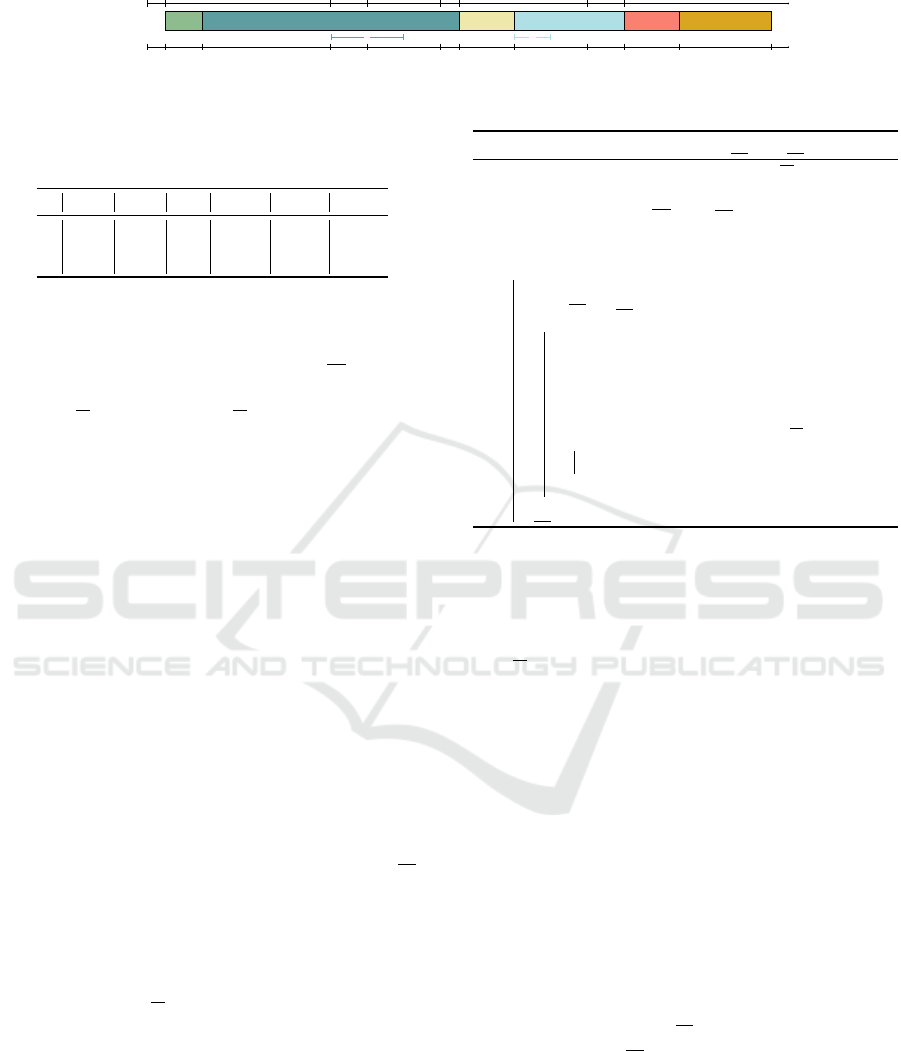
3 1 6 5 4 2

1 5

, d

0 1 3 10 12 16 17 20 24 26 29 34

2 3 -3 4 5 6 -1 -5

Figure 2: An optimal schedule of the instance of Table 1 for the 1|r

∑

problem, where

∑

= 129.

Table 2: Domains of the S

variables and the corresponding

′

and d

′

values.

′

1 2 3 4 5 6

[0, 10] [0, 46] [1, 8] [12, 49] [16, 20] [17, 17]

′

0 0 1 12 16 17

′

24 51 10 51 26 20

[100,130].

A solution of this relaxation is described in Fig-

ure 3. The value of the lower bound, F

′

found by

the relaxation is 104, it is more than 100, the current

value of F, so the value of F is updated to 104. It

can be noticed that since the 1|r

; pmtn|

∑

relax-

ation does not enforce the respect of the deadlines,

task 1 is late. In the same way, since the respect of

the mandatory parts of the tasks is not a constraint of

1|r

; pmtn|

∑

, some tasks are not executed on their

mandatory part even if they should. This observation

is also true for ﬁxed tasks. This is the reason why the

integration of mandatory parts will also be evaluated.

4.3 Filtering the Bounds of the Domains

of the Start Time Variables

The second ﬁltering rule of flowtime updates the

bounds of the domain of the start time variables, S

For sake of simpliﬁcation, only the ﬁltering of the

lower bounds is presented. The algorithm for ﬁlter-

ing the upper bounds is symmetric to Algorithm 1.

For each T

′

, the algorithm schedules T

′

without

preemption from its earliest starting time (i.e. S

This time is noted t in the following. It then tries to

schedule the other tasks around T

′

following the solv-

ing algorithm of the relaxation. The optimality proof

of schedule for the relaxation with T

′

ﬁxed is similar

to those for the mandatory parts (Bonnin et al., 2022).

If the objective value found by the relaxation is

strictly bigger that F, then there is no feasible solution

for which T

′

begins at time t and t is ﬁltered from the

domain of S

. Indeed, as the objective value found by

the relaxation is a lower bound of F if T

′

begins at

time t, then a similar reasoning than what is done in

Section 4.2 can be made.

It can also happen that the relaxation does not have

a solution. For instance, if T

′

is scheduled on the

mandatory part of another task and the relaxation en-

Algorithm 1: Filtering algorithm of S

, . . . , S

Data: {S

, . . . , S

}, {p

, . . . , p

}, F

Result: Updated {S

, . . . , S

}

′

, . . . , T

′

} ← the tasks created from {S

. . . , S

} and {p

, . . . , p

};

for j ← 1 to n do

t ← S

;

while t ≤ S

relax

j,t

← value of the objective

found by solving the relaxation

while setting T

′

to be executed in [t,

t + p

];

if relax

j,t

= ∅ or relax

j,t

> F then

t ← t + 1;

else break;

← t

sure the respect of mandatory parts. In this case, there

is no feasible solution for which T

′

begins at time t, t

is then ﬁltered from the domain of S

In the other case, if there is a solution and the ob-

jective value computed by the relaxation is no bigger

than F, a support can be found in which T

′

begins at

time t, so no deduction is made. It is then not possible

to ﬁlter more the lower bound of S

, so the algorithm

stops for this task and start looking at the next task.

Proposition 3. The complexity of Algorithm 1 is O(n ·

M ·R) where M = max

(|S

|) and R is the complexity

of the relaxation algorithm.

Proof. Creating one task T

′

is an O(1) operation. It

is repeated for each of the n tasks to be created. So

the ﬁrst line has an O(n) complexity.

For the loop, the action is repeated for all n tasks.

The ﬁrst and last line of the for loop are assigna-

tions that take O(1), so the complexity is bounded

by the complexity of the while loop. The while loop

is repeated at most for all possible values of the do-

main of S

(from S

to S

), and so at a maximum

of M = max

(|S

|) times. Setting the task to be ex-

ecuted in [t,t + p

] and computing the relaxation can

be done with the same complexity R as simply com-

puting the relaxation by the same argument as what

is done in (Bonnin et al., 2022). The if and else parts

are only simple tests and assignations and so have an

O(1) complexity. The complexity of the for loop is

Toward a Global Constraint for Minimizing the Flowtime

2 3 2 1 4 1 5 6 5 1

1 56

, d

0 1 3 7 12 15 16 17 20 25 33

2 3 -3 4 5 6 -6 -1 -5

Figure 3: An optimal solution of the 1|r

; pmtn|

∑

relaxation for the T

′

tasks, where

∑

= 104.

then bound by O(n · M ·R).

The complexity of Algorithm 1 is then bound by

O(n · M · R) where M = max

(|S

|) and R is the com-

plexity of the relaxation algorithm.

Example 4 (Execution of Algorithm 1). This exam-

ple uses the same values as Example 2 and only the

ﬁltering of S

is given. Figure 4 shows the results of

the relaxation at each step of the algorithm. At steps

1, 2, and 3, where t = 0, 1, and 2 respectively, the ob-

jective value of the relaxation is strictly greater than

those of F, 130. So the value of S

is updated to 3. But

at step 4, where t = 3, the objective value of the relax-

ation is no greater than 130, it is not possible to ﬁlter

more the value of S

and the algorithm stops looking

at T

′

and begins examining the next task.

A choice is made in Algorithm 1 to only ﬁlter the

bounds of the S

variables as a classical representation

of a task in constraint programming is an interval vari-

able for which most of the solvers only allow bounds

ﬁltering. Algorithm 1 is a naive version of a ﬁlter-

ing rule for flowtime as it tests each possible value

for S

. Once the promising relaxations are identiﬁed,

speciﬁc rules or algorithms should be designed for

those relaxations. To obtain the complete ﬁltering al-

gorithm of the flowtime constraint, the bound update

of Section 4.2 must be executed ﬁrst. Then, if there

is no contradiction with F, the lower bounds of the

variables must be updated with Algorithm 1 and

the last step is to update the upper bounds of the S

variables with a symmetric algorithm to Algorithm 1.

5 EXPERIMENTAL RESULTS

This section aims to evaluate the relaxations and ﬁlter-

ing rules available for the global constraint flowtime.

The experiment framework is deﬁned so the follow-

ing questions are addressed: Q1. Which relaxation is

the best proving the optimality or ﬁnding good upper

bounds? Q2. What are the performance trade-offs be-

tween the propagation of the lower bound and the ﬁl-

tering of the starting times? In terms of solving time?

Number of branches? Q3. What is the efﬁciency of

the constraint depending on the problem?

Section 5.1 describes the experimental protocol

with the alternatives for the flowtime constraint. The

constraint is evaluated on two ﬂowtime minimization

problems: a single machine problem in Section 5.2;

and a permutation ﬂowshop problem in Section 5.3.

5.1 Experimental Protocol

The following alternatives are considered for the

global constraint flowtime: sum uses a stan-

dard sum constraint for propagating the ﬂowtime;

pmtnFlow propagates the lower bound as presented

in Section 4.2 using 1|r

; pmtn|

∑

; pmtnBusy

propagates the lower bound using 1|r

; pmtn|

∑

;

mandFlow propagates the lower bound using

1|r

; pmtn; mand|

∑

; mandBusy propagates

the lower bound using 1|r

; pmtn; mand|

∑

;

norelFlow propagates the lower bound using

1|d

∑

; filtFlow does as pmtnFlow but also

ﬁlters the starting times as presented in Sec-

tion 4.3 using 1|r

; pmtn|

∑

; filtBusy does

as pmtnBusy and ﬁlters the starting times using

1|r

; pmtn|

∑

; complBusy adapts the Completion

constraint (Kov

acs and Beck, 2011), which uses

1|r

; pmtn|

∑

, as described in the following.

The proposed alternatives have been implemented

as a global constraint in C++ and embedded into

IBM ILOG CPLEX Optimization Studio 22.1 (IBM,

2023). All models state the standard sum constraint

and a noOverlap constraint. The noOverlap con-

straint sets the resource capacity enforcement and

uses the default inference techniques.

The Completion constraint proposed in (Kov

acs

and Beck, 2011, complBusy) has been made com-

patible with the latest version of CP Optimizer with

the minimum possible changes on the code. Indeed,

the IlcActivity type is not available anymore because

it has been replaced by IloIntervalVar. IlcActivity

allowed to remove values from an enumerated do-

main, creating holes, but IloIntervalVar only accepts

changes on the bounds of its interval domain. The

Completion constraint has then been adapted to use

IloIntervalVar variables instead of IlcActivity ones.

Therefore, keep in mind that the original constraint

has been weakened as it only updates the bounds of

the domains. For the same reason, the version tested

is not optimized, so the time results for complBusy

should be read as upper bounds and not precise mea-

sures.

ICORES 2024 - 13th International Conference on Operations Research and Enterprise Systems

1 3 4 6 2 5

1 56

, d

0 14 16 19 22 27 33

2 3 -3 4 5 6 -1 -5

(a) Step 1 : t = 0, relax

1,0

= 131 > 130(= F) : 0 can be ﬁltered from the domain of S

2 1 3 6 4 2 5

1 56

, d

0 1 15 17 20 23 27 33

2 3 -3 4 5 6 -1 -5

(b) Step 2 : t = 1, relax

1,1

= 135 > 130(= F) : 1 can be ﬁltered from the domain of S

2 3 1 3 6 4 2 5

1 56

, d

0 1 2 16 17 20 23 27 33

2 3 -3 4 5 6 -1 -5

1,2

= 136 > 130(= F) : 2 can be ﬁltered from the domain of S

2 3 1 6 4 2 5

1 56

, d

0 1 3 17 20 23 27 33

2 3 -3 4 5 6 -1 -5

(d) Step 4 : t = 3, relax

1,3

= 123 ≤ 130(= F) : STOP, a support of S

has been found.

Figure 4: Example of the ﬁltering rule of the lower bound of S

variable (second rule) with the 1|r

; pmtn|

∑

relaxation.

The example uses the instance of Table 2 and S

, whose previous value was 0, is updated to 3.

Only results obtained using a CP model are pre-

sented as results obtained by implementing a classical

MIP time-indexed model (Keha et al., 2009) with the

same conﬁguration are always at least 2 times slower

than those obtained using the sum alternative.

All experiments were run on a Dell computer with

256 GB of RAM and 4 Intel E7-4870 2.40 GHz pro-

cessors running on CentOS Linux release 7.9 (each

processor has 10 cores). The parallelism is disabled

in order to ease the comparative analysis. Last, the

time limit is 1000 seconds for each run.

5.2 Single Machine Problem

The problem instances for the single machine prob-

lem have been proposed in (Pan and Shi, 2008)

for 1|r

∑

and also used in (Kov

acs and Beck,

2011). The repository contains 10 problem instances

for each combination of parameters n and R, where n

is the number of tasks, while R is the relative range of

the release date. We have selected all 900 instances

with fewer than 100 tasks for every relative range.

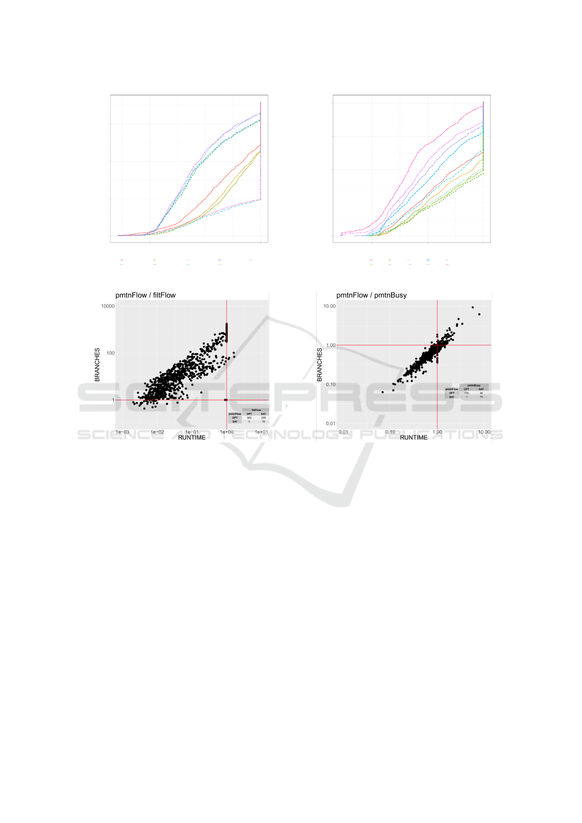
Figure 5a gives the number of instances optimally

solved depending on the time grouped by alternative.

All instances that have reached the time limit are in

the vertical line at time 1e +03. A faster alternative is

above and on the left of a slower alternative. Clearly,

the alternatives sum and norelFlow are the worst al-

ternatives because they only optimally solve around

250 instances over 900 and are an order of magnitude

slower than the other alternatives. So, the alternative

norelFlow can be discarded as inefﬁcient in future

work. The alternatives that ﬁlter the starting times im-

prove the efﬁciency by optimally solving more than

500 instances. The alternative filtBusy is slightly

faster than filtFlow, and they are both slightly less

efﬁcient and slower than complBusy. It shows an in-

terest in the incrementality of the ﬁltering compared

to our more naive, but simpler, approach. Currently,

the alternatives that only propagate the lower bound

are the most efﬁcient and the fastest. Surprisingly, the

integration of the mandatory part does not give any

signiﬁcant improvement. To conclude, pmtnFlow is

the most efﬁcient closely followed by pmtnBusy. Fil-

tering the starting times takes too much time and leads

to fewer optimality proofs even when the ﬁltering is

incremental as in complBusy.

Figure 5b gives the number of instances optimally

solved depending on the time it took grouped by the

relative range R of the release dates. The relative

Toward a Global Constraint for Minimizing the Flowtime

250

500

750

1e−01 1e+01 1e+03

RUNTIME

Count

complBusy

filtBusy

filtFlow

mandBusy

mandFlow

norelFlow

pmtnBusy

pmtnFlow

sum

(a) Alternatives survival plot.

200

400

600

800

1e−01 1e+01 1e+03

RUNTIME

Count

0.20

0.40

0.60

0.80

1.00

1.25

1.50

1.75

2.00

3.00

(b) Relative range survival plot.

Figure 5: Experimental results for the single machine problem.

range is relevant with respect to the problem hard-

ness because the curves can be easily distinguished.

The easiest instances have the greatest ranges (3.00,

2.00, 1.75, 1.50, 1.25) because, for a given time win-

dow, only a few tasks overlap, reducing the degree

of freedom for scheduling. Then, instances that have

the lowest ranges (0.20, 0.40) are also pretty easy, be-

cause the problem becomes close to 1||

∑

and the

relaxation is likely to give good lower bounds. Fi-

nally, the middle ranges (0.60, 0.80, 1.00) lead to the

hardest instances because the relaxation is weaker and

the degree of freedom for scheduling remains high.

In Figures 5c and 5d, each point represents one in-

stance and its x coordinate is the ratio of the solving

time of the ﬁrst alternative over the solving time of

the second alternative, whereas its y coordinate is the

ratio of the branches. Notice also that both scales are

logarithmic. All points located above and on the right

of the point (1,1) are instances improved by the sec-

ond alternative. On the contrary, all points located be-

low and on the left of the point (1,1) are instances im-

proved by the ﬁrst alternative (bottom-left quadrant).

As expected, all points are around the diago-

nal as the number of nodes is roughly proportional

to the time (top-left and bottom-right quadrants are

empty). Figure 5c shows that ﬁltering the starting

times (filtFlow) reduces by an order of magnitude

on the number of branches compared to the propa-

gation of the lower bound (pmtnFlow), but it is so

slow that the solving time remains larger by an order

of magnitude. Therefore, ﬁltering the starting times

is promising, but this requires further improvements

beyond the incrementality.Figure 5d shows that the

relaxation with the ﬂowtime gives more optimality

proofs, explores fewer branches and is faster than the

relaxation with the mean busy time.

Table 3 summarizes the experimental results as in

(Kov

acs and Beck, 2011). Each row contains com-

bined results for the 10 instances with the same num-

ber of activities, n, and release time range, R. For

ICORES 2024 - 13th International Conference on Operations Research and Enterprise Systems

Table 3: Experimental results for four alternatives on single machine problems.

Problem sum pmtnFlow filtFlow complBusy

n R o b t o b t o b t o b t

20 0.2 – – – 10 14.7K 0.3 10 0.8K 1.8 10 0.9K 0.1

0.6 3 10.0M 292.5 10 23.8K 0.5 10 2.8K 5.2 10 8.7K 3.2

1.0 10 1.9M 57.1 10 14.6K 0.3 10 6.1K 8.7 10 9.0K 2.7

1.5 10 81.4K 2.0 10 7.5K 0.2 10 2.2K 3.4 10 4.2K 0.8

2.0 10 9.2K 0.2 10 5.6K 0.1 10 1.9K 1.4 10 2.8K 0.5

30 0.2 – – – 10 30.1K 0.9 10 1.5K 10.3 10 3.5K 1.7

0.6 – – – 10 43.0K 1.2 10 3.9K 26.1 10 16.5K 19.3

1.0 2 2.5M 101.4 10 45.6K 1.6 10 16.2K 69.2 10 25.9K 37.8

1.5 9 494.7K 17.7 10 11.2K 0.3 10 5.4K 15.6 10 9.4K 2.2

2.0

10 81.3K 2.7 10 10.2K 0.3 10 5.3K 14.0 10 7.8K 1.1

40 0.2 – – – 10 34.0K 1.4 10 3.0K 44.1 10 13.5K 12.5

0.6 – – – 10 94.4K 4.1 10 8.2K 116.3 10 82.4K 90.5

1.0 2 7.5M 368.8 10 43.7K 2.0 10 12.9K 82.0 10 44.0K 19.9

1.5 10 1.4M 64.8 10 13.8K 0.5 10 7.5K 38.7 10 23.8K 6.4

2.0 9 191.4K 7.8 10 13.1K 0.5 10 5.8K 27.8 10 10.4K 8.8

50 0.2 – – 10 52.4K 3.7 10 6.3K 171.8 10 48.6K 39.5

0.6 – – – 10 213.8K 12.3 8 14.5K 383.1 10 282.5K 291.1

1.0 – – – 10 2.2M 143.8 5 31.9K 423.1 5 199.7K 331.7

1.5 4 2.5M 118.6 10 70.2K 4.4 10 18.8K 168.7 10 75.3K 158.0

2.0 8 630.0K 31.3 10 18.6K 0.9 10 8.1K 74.0 10 18.0K 10.49

60 0.2 – – – 10 109.1K 9.1 6 10.8K 517.0 8 150.8K 239.2

0.6 – – – 10 1.3M 107.1 2 12.9K 662.9 – – –

1.0 – – – 9 342.1K 26.3 6 21.9K 528.2 3 150.7K 784.3

1.5 – – – 10 32.6K 2.2 10 16.3K 199.4 10 36.8K 32.5

2.0 6 3.7M 187.6 10 24.0K 1.2 10 6.8K 88.9 10 41.4K 14.7

70 0.2 – – – 10 430.1K 40.0 3 10.1K 674.8 3 69.7K 632.1

0.6 – – – 8 2.7M 267.1 – – – – – –

1.0 – – – 10 2.1M 192.0 2 38.1K 831.4 2 197.3K 332.3

1.5 – – – 10 119.1K 10.1 8 26.0K 488.0 9 174.7K 215.1

2.0 3 5.2M 312.2 10 41.0K 2.7 10 20.3K 291.1 10 52.8K 55.0

each of the 4 alternatives, the table displays the num-

ber of instances that were solved to optimality (col-

umn o), the average number of branches (b), and the

average search time in seconds (t). The averages are

computed only on the instances that the algorithm op-

timally solved. Table 3 conﬁrms that the 3 alternatives

for the flowtime constraint are more efﬁcient and re-

duce the number of branches compared to the sum

constraint. More and larger instances are optimally

solved in Table 3 than in (Kov

acs and Beck, 2011)

where only a few instances with 50 tasks or more are

optimally solved. The comparison between the prop-

agation of the lower bound (pmtnFlow) and the ﬁlter-

ing of the starting times (filtFlow and complBusy)

also differs. In (Kov

acs and Beck, 2011), the ﬁl-

tering of the starting times outperforms the propa-

gation of the lower bound in terms of the number

of optimality proofs, solving times, and number of

branches. The reason is not obvious, but could in-

clude the change of objective function, or our adapta-

tion of the completion constraint.

The detailed results are not given here, but the sit-

uation is similar when comparing the upper bounds

on instances that are not optimally solved.

To conclude on the single machine, 1|d

∑

is not efﬁcient, but other preemptive relaxations are

more efﬁcient in terms of solving time and reducing

the number of branches, with a slight advantage for

the ﬂowtime over the mean busy time. Mandatory

parts do not have much practical importance for ﬁl-

tering the starting times. Still, the results obtained

using 1|d

∑

and, to some extent, the mandatory

part might be biased due to instances lacking dead-

lines. Last, ﬁltering the starting times is not yet efﬁ-

cient enough to balance the additional time required

for it compared to the lower bound propagation. Yet,

it drastically reduces the number of branches which

is promising for designing more efﬁcient algorithms

through incrementality and triggering.

5.3 Flowshop Problem

The ﬂowshop problem consists of determining a pro-

cessing sequence of n tasks in a set of m machines

that are arranged in series. All tasks must be pro-

cessed sequentially in all machines. Each task needs

a given processing time at each machine. A ﬂowshop

is a common production setting in factories where

products start processing at machine or stage 1 and

continue processing until they are ﬁnished in the last

machine. The permutation ﬂowshop problem also as-

sumes that the production sequence of tasks for the

ﬁrst machine is kept unaltered for all other machines.

The 300 instances have between 5 and 20 ma-

Toward a Global Constraint for Minimizing the Flowtime

chines: 60 instances of (Taillard, 1993) have between

20 and 50 jobs; and 240 instances of (Vallada et al.,

2015) have between 10 and 60 jobs. Table 4 and Ta-

ble 5 present the experimental results for the ﬂowshop

for ﬁve relevant alternatives identiﬁed in Section 5.2.

Table 4 gives for each alternative the number of in-

stances solved optimally, the average search time (in

seconds), the average number of branches, and their

standard deviations. Those last four values are com-

puted over the optimally solved instances only, other-

wise, the time limit is reached and these are not sig-

niﬁcant. It shows that the improvement provided by

the global constraint is not as signiﬁcant as for the sin-

gle machine problem. In fact, pmtnFlow is the quick-

est to prove the optimality, followed by complBusy

and pmtnBusy, then sum and filtFlow is the one that

takes the longest by far. However, pmtnFlow is doing

one fewer proof than complBusy, pmtnBusy, and sum,

and filtFlow is doing very fewer proofs than the oth-

ers. In terms of the number of branches, filtFlow is

doing smaller proofs, but as it does less than 3/5 of

the proofs done by the other alternatives, the compar-

ison is hard to do. As expected, for the other alterna-

tives, complBusy is the one with the fewer branches,

followed by pmtnFlow, then pmtnBusy, and by far

sum. Note that at most 36 instances over 300 are op-

timally solved as even the smallest ﬂowshop instance

has more operations (100) than the bigger instances

tested for the single machine problem.

Table 4: Time and number of branches per alternative.

Alternative Opt Time (s) Branches

a o avg std avg std

sum 36 317 269 2.26M 1.60M

pmtnBusy 36 257 244 1.86M 1.43M

pmtnFlow 35 237 228 1.67M 1.25M

complBusy 36 257 231 1.28M 1.03M

filtFlow 21 412 336 0.54M 0.46M

Table 5 summarizes the relative error of each al-

ternative over all instances. The relative error for an

instance is the ratio of the absolute error to the best

known objective value for this instance. For each al-

ternative (column a), the table displays the number

of the instances optimally solved (column o), the av-

erage relative error (avg), and its standard deviation

(std) in per-thousand. The averages are computed

over all 300 instances. For the relative error, the al-

ternative sum gives the best results closely followed

by pmtnBusy, and less closely by pmtnFlow. The ﬁl-

tering of the starting times gives signiﬁcantly worse

upper bounds (complBusy and mostly filtFlow).

A possible explanation is that the instances for the

ﬂowshop problem are larger and harder than those for

the single machine so the search speed becomes more

Table 5: Mean relative error (over all instances).

a o avg (‰) std (‰)

sum 36 0.48 0.63

pmtnBusy 36 0.50 0.66

pmtnFlow 35 0.55 1.19

complBusy 36 1.35 2.18

filtFlow 21 5.01 4.76

important than the propagation strength for ﬁnding

good upper bounds. Furthermore, many scheduling

decisions, even for the permutation ﬂowshop, have

less inﬂuence over the relaxation because they con-

cern earlier machines. Indeed, the schedule of the last

machine entirely determines the ﬂowtime and it de-

pends on the schedule of all previous machines, giv-

ing less visibility to the bound and the ﬁltering. It

shows that even the propagation of the lower bound

should be more carefully triggered to save time and

that ﬁltering the relative order of tasks could help as

in most global constraints for scheduling.

To conclude this section, the flowtime constraint

helps to improve the performances of the solver on

single machine problems. However those results do

not carry to more complex scheduling problems like

the ﬂowshop problem. The main part to improve is the

ﬁltering part as it considerably reduces the number of

branches, but currently takes too much time.

6 CONCLUSIONS

This article proposes a global constraint minimizing

the ﬂowtime that allows using multiple polynomial

relaxations of 1|r

∑

. For now, the flowtime

constraint is more efﬁcient than a standard sum con-

straint on a single machine problem but only has a

moderate effect on the ﬂowshop problem. The exper-

imental results have identiﬁed the most efﬁcient re-

laxations and shown that ﬁltering the starting times

takes too long to improve the solving times despite

reducing the number of branches.

This work opens new perspectives for designing

more efﬁcient ﬁltering rules and algorithms for the

flowtime constraint. First, incremental ﬁltering of

the starting times would improve the performances

but is not enough for compensating the additional

time. Second, the events that trigger the ﬁltering are

key to efﬁciency because most of the ﬁltering stages

do not reduce the domains. Third, the detection of

precedences between tasks may strengthen the ﬁlter-

ing while reducing the number of steps as in the dis-

junctive constraint. Finally, the last avenue is to inte-

grate the last untested relaxation 1|sp-graph|

∑

that is not solved by a priority list algorithm.

ICORES 2024 - 13th International Conference on Operations Research and Enterprise Systems

ACKNOWLEDGEMENTS

We thank Andr

as Kov

acs and J. Christopher Beck for

sharing their code, and the latter for his advice.

REFERENCES

Aggoun, A. and Beldiceanu, N. (1993). Extending chip

in order to solve complex scheduling and placement

problems. Math Comput Model.

Awerbuch, B., Azar, Y., Leonardi, S., and Regev, O. (2002).

Minimizing the ﬂow time without migration. SIAM J

Comput.

Baptiste, P., Laborie, P., Pape, C. L., and Nuijten, W. (2006).

Constraint-based scheduling and planning. In Rossi,

F., van Beek, P., and Walsh, T., editors, Handbook

of Constraint Programming, Foundations of Artiﬁcial

Intelligence. Elsevier.

Baptiste, P., Le Pape, C., and Nuijten, W. (2001a).

Constraint-based scheduling: applying constraint

programming to scheduling problems. Springer Sci-

ence & Business Media.

Baptiste, P., Le Pape, C., and Nuijten, W. (2001b).

Constraint-based scheduling: applying constraint

programming to scheduling problems. Int Ser Oper

Res Man. Springer.

Bewoor, L. A., Prakash, V. C., and Sapkal, S. U. (2018).

Production scheduling optimization in foundry using

hybrid particle swarm optimization algorithm. Proce-

dia Manuf.

Bonnin, C., Nattaf, M., Arnaud, A. M., and Espinouse, M.-

L. (2022). Extending smith’s rule with task mandatory

parts and release dates. In PMS 2022.

Brucker, P. (2004). Single Machine Scheduling Problems.

Springer Berlin, Heidelberg.

Carlier, J. (1982). The one-machine sequencing problem.

Eur J Oper Res.

Carlier, J. and Pinson,

E. (1990). A practical use of jack-

son’s preemptive schedule for solving the job shop

problem. Ann Oper Res.

Chen, B., Potts, C. N., and Woeginger, G. J. (1998). A Re-

view of Machine Scheduling: Complexity, Algorithms

and Approximability. Springer US.

Cho, B.-H., Athar, H. M., Bates, L. G., Yarnoff, B. O., Har-

ris, L. Q., Washington, M. L., Jones-Jack, N. H., and

Pike, J. J. (2023). Patient ﬂow time data of covid-19

vaccination clinics in 23 sites, united states, april and

may 2021. Vaccine.

Du, J. and Leung, J. Y. (1993). Minimizing mean ﬂow time

with release time and deadline constraints. J Algo-

rithm.

Fahimi, H. and Quimper, C.-G. (2014). Linear-time ﬁltering

algorithms for the disjunctive constraint. Proceedings

of the AAAI Conference on Artiﬁcial Intelligence.

Focacci, F., Lodi, A., and Milano, M. (1999). Cost-based

domain ﬁltering. In Jaffar, J., editor, Lect Notes Com-

put SC. Springer Berlin Heidelberg.

Gay, S., Hartert, R., and Schaus, P. (2015). Simple and scal-

able time-table ﬁltering for the cumulative constraint.

In Pesant, G., editor, Lect Notes Comput SC. Springer

International Publishing.

Graham, R., Lawler, E., Lenstra, J., and Kan, A. (1979).

Optimization and approximation in deterministic se-

quencing and scheduling: a survey. In Hammer, P.,

Johnson, E., and Korte, B., editors, Discrete Optim II,

Annals of Discrete Mathematics. Elsevier.

IBM (2023). Cplex optimisation studio 22.1. https://www.

ibm.com/products/ilog-cplex-optimization-studio.

Keha, A., Khowala, K., and Fowler, J. (2009). Mixed in-

teger programming formulations for single machine

scheduling problems. Comput Ind Eng.

Kov

acs, A. and Beck, J. C. (2011). A global constraint for

total weighted completion time for unary resources.

Constraints.

Labetoulle, J., Lawler, E., Lenstra, J., and Rinnooy Kan, A.

(1984). Preemptive scheduling of uniform machines

subject to release dates. In Progress in combinatorial

optimization. Academic Press.

Lahrichi, A. (1982). Ordonnancements. la notion de parties

obligatoires et son application aux probl

emes cumu-

latifs. RAIRO-Oper Res.

Lawler, E. (1978). Sequencing jobs to minimize total

weighted completion time subject to precedence con-

straints. In Alspach, B., Hell, P., and Miller, D., ed-

itors, Algorithmic Aspects of Combinatorics, Ann. of

Discrete Math. Elsevier.

Lenstra, J., Rinnooy Kan, A., and Brucker, P. (1977). Com-

plexity of machine scheduling problems. Ann. of Dis-

crete Math.

Lenstra, J. K. (accessed in 2023). Unpublished. http:

//schedulingzoo.lip6.fr/ref2bibtex.php?ID=Lenstra::.

Lenstra, J. K. and Rinnooy Kan, A. (1978). Complexity of

scheduling under precedence constraints. Oper Res.

Letort, A., Beldiceanu, N., and Carlsson, M. (2012). A scal-

able sweep algorithm for the cumulative constraint. In

Milano, M., editor, Lect Notes Comput SC. Springer

Berlin Heidelberg.

Pan, Y. and Shi, L. (2008). New hybrid optimization al-

gorithms for machine scheduling problems. IEEE T

Autom Sci Eng.

Pinedo, M. L. (2012). Scheduling: theory, algorithms, and

systems. Springer New York, NY.

Stewart, R., Raith, A., and Sinnen, O. (2023). Optimising

makespan and energy consumption in task scheduling

for parallel systems. Comput Oper Res.

Strusevich, V. A. (2022). Complexity and approximation of

open shop scheduling to minimize the makespan: A

review of models and approaches. Comput Oper Res.

Taillard,

E. (1993). Benchmarks for basic scheduling prob-

lems. Eur J Oper Res.

Vallada, E., Ruiz, R., and Framinan, J. M. (2015). New hard

benchmark for ﬂowshop scheduling problems min-

imising makespan. Eur J Oper Res.

Vil

ım, P. (2004). O(nlogn) ﬁltering algorithms for unary

resource constraint. In R

egin, J.-C. and Rueher, M.,

editors, Lect Notes Comput SC. Springer Berlin Hei-

delberg.

Toward a Global Constraint for Minimizing the Flowtime