Lens Flare-Aware Detector in Autonomous Driving
Shanxing Ma
a
and Jan Aelterman
b
TELIN-IPI, Ghent University – imec, Sint-Pietersnieuwstraat, Ghent, Belgium
Keywords:
Autonomous Driving, Object Detection, Bayes’ Theorem, Lens Flare.
Abstract:
Autonomous driving has the potential of reducing traffic accidents, and object detection plays a key role. This
paper focuses on the study of object detection in the presence of lens flare. We analyze the impact of lens flare
on object detection in autonomous driving tasks and propose a lens flare adaptation method based on Bayesian
reasoning theory to optimize existing object detection models. This allows us to adjust the detection scores
to re-rank the detections of detection models based on the intensity of lens flare and achieve a higher average
precision. Furthermore, this method only requires simple modifications based on the detection results of the
existing object detection models, making it easier to deploy on existing devices.
1 INTRODUCTION
Automated Driving Systems (ADSs) are being devel-
oped to prevent accidents, reduce emissions, transport
the mobility-impaired, and reduce driving-related
stress (Crayton and Meier, 2017). According to
the National Highway Traffic Safety Administration
(NHTSA), 94% of road accidents are caused by hu-
man error (Singh, 2015). For this reason, many al-
gorithms have been developed, for example, object
detection & tracking, and path planning, to support
a higher level of ADSs. Object detection is a funda-
mental but important component in autonomous driv-
ing. The performance of object detection directly im-
pacts the performance of downstream tasks. There-
fore, research on object detection has received sig-
nificant attention. Especially in ADSs, the complex-
ity and diversity of realistic scenarios have presented
more challenges to object detection algorithms, in-
cluding adverse weather conditions, low-light and ex-
tremely high-light situations, and severe occlusion be-
tween objects.
IEEE P2020 Automotive Imaging White Paper
mentioned an optical artifact caused by the lens in a
camera system, which is lens flare. In the automotive
use environment, headlamps direct light and/or direct
sunlight often enter the Field of View (FoV) or hit
the optics of the camera system. Stray light of inci-
dent light onto the optical system shall be evaluated
in terms of the veiling effect that deteriorates image
a
https://orcid.org/0000-0001-5650-0168
b
https://orcid.org/0000-0002-5543-2631
visual or post-processing performance (Group et al.,
2018). However, to the best of the author’s knowl-
edge, there are currently no articles focusing on the
impact of lens flare on object detection in autonomous
driving scenarios.
In this paper, we aim to enhance the object de-
tection performance of existing detectors in scenarios
with lens flare by using Bayesian reasoning theory.
First, we generated an autonomous driving dataset
with added lens flares. Then we proposed a lens flare-
aware belief calibration algorithm based on Bayesian
reasoning theory, which can be easily deployed on top
of the existing object detection models. We consider
that the actual distribution of True Positive (TP) and
False Positive (FP) is not strictly positively or nega-
tively correlated with the predicted confidence scores
when different intensity of lens flare occurs. There-
fore, when we consider the effects of lens flare, we
can calibrate the confidence score (enhanced or weak-
ened) according to their intensities to achieve better
performance.
Figure 1 illustrates the proposed method, which
consists of three parts, an object detector module, a
lens flare perception module, and a belief adaptation
modification module. The images captured by the
camera are sent to the object detector. Then the object
detector outputs the initial detection results, including
the confidence score, class, and position of each ob-
ject, which will be fed into the lens flare perception
module to calculate the lens flare intensity of each
detected object. Finally, the belief adaptation modi-
fication module calibrates only the confidence score
Ma, S. and Aelterman, J.
Lens Flare-Aware Detector in Autonomous Driving.
DOI: 10.5220/0012309900003660
In Proceedings of the 19th International Joint Conference on Computer Vision, Imaging and Computer Graphics Theory and Applications (VISIGRAPP 2024) - Volume 2: VISAPP, pages
341-348
ISBN: 978-989-758-679-8; ISSN: 2184-4321
Copyright © 2024 by Paper published under CC license (CC BY-NC-ND 4.0)
341

Figure 1: The proposed method is composed of three parts. The object detector can be any pre-trained object detection
network, such as YOLO. The lens flare perception module can estimate the intensity of the lens flare for each detected object.
The belief adaptation modification module then maps the confidence score into the log-likelihood ratio value based on the
estimated lens flare intensity.
according to the intensity of lens flare and outputs the
final detection result.
2 RELATED WORK
2.1 Object Detection
Object detection has become a fundamental and im-
portant part not only in ADSs but also in computer
vision tasks. Due to the excellent performance of
deep learning in object detection, most of the re-
cently published papers are based on deep learning
models. They can be mainly divided into two cate-
gories: the region proposal-based methods and one-
stage regression-based methods (Liu et al., 2022).
The former methods first find the Region of Interest
(RoI), and then classify them into different classes,
representative methods include Fast R-CNN (Gir-
shick, 2015) and Faster R-CNN (Ren et al., 2015).
The latter methods output the final detection result
through one network, representative methods include
YOLO (Redmon et al., 2016; Jocher et al., 2022)and
SSD (Liu et al., 2016). Due to the success of the
Transformer model in natural language processing,
some researchers have tried to explore the application
of the Transformer to object detection tasks, such as
Vision Transformer (Dosovitskiy et al., 2020).
2.2 Object Detection in Adverse
Conditions
In autonomous driving tasks, adverse conditions have
been regarded as a huge obstacle to solve. The meth-
ods in this field can be mainly divided into two cate-
gories. One approach involves direct modifications to
the neural network architecture, where both clear and
adverse condition images are incorporated for net-
work retraining (Hnewa and Radha, 2020). In con-
trast, other researchers opt to include an additional
preprocessing module for improving adverse condi-
tion image quality before feeding them into a conven-
tional network (Liu et al., 2022). Most of them only
focus on one specific problem and achieve better per-
formance on this task, such as fog (Liu et al., 2022),
haze (Yu et al., 2022), and low light (Rashed et al.,
2019). Some researchers try to solve all of these prob-
lems with a unified model (Chen et al., 2022), which
gives readers some new aspirations. However, there
are still many issues in autonomous driving tasks that
have not been noticed and well addressed, lens flare
is one of them. To the best of the author’s knowledge,
no research has been done focusing on lens flare in
object detection in autonomous driving scenarios.
2.3 Lens Flare
Most of the work done on lens flare is about image
quality enhancement (Rashed et al., 2019; Talvala
et al., 2007). They can eliminate some lens flares in
simple scenarios, but for some complex scenarios or
severe lens flares, the results of these methods are not
acceptable. To fully utilize the power of deep learn-
ing, two lens flare datasets released recently give re-
searchers more flexibility. One is the daytime lens
flare dataset (Wu et al., 2021), which only consists of
the sun’s lens flare, and another is the nighttime lens
flare dataset (Dai et al., 2022), which only consists of
the colored light sources’ lens flare. Our paper also
uses these two datasets to generate an autonomous
driving dataset with added lens flares.
VISAPP 2024 - 19th International Conference on Computer Vision Theory and Applications
342

3 METHODOLOGY
In this section, we will describe the methodology and
experimental setup in detail. Due to the fact that the
original output of the object detector is globally op-
timal and does not specifically optimize for different
intensities of lens flare, we adopt the Bayesian reason-
ing theory to calibrate the output of the object detector
based on the intensities of lens flare.
More specifically, for a given intensity of lens
flare, we can calculate the distribution of positive
and negative samples accordingly. This allows us to
map the detection scores into statistical scores, specif-
ically the Log-Likelihood Ratio (LLR), which pro-
vides a more accurate reflection of the network’s per-
formance across varying intensities of lens flare. This
approach aims to improve the detection performance
in the presence of lens flare and can be easily de-
ployed on top of different existing object detectors
with only little effort.
3.1 Theoretical Foundation
When an object of interest, i.e. the object belonging
to the category that the detector is trained to predict,
is detected by the detector, the output can be defined
as z
k
= (u
k
, s
k
, a
k
). In z
k
, u
k
is the location, s
k
is the
size, and a
k
∈ (0, 1) is the confidence score, of the k-th
output of the detector in a sensor-specific coordinate
system.
A road user, such as a vehicle or pedestrian, (x,g)
is a tuple containing the position x of the road user
in the world coordinate and the feature g which de-
scribes the road user in a more detail way, such color,
size, shape, etc.
Then we use hypothesis H
1
(x, g) to define a road
user with feature g present at location x, and the out-
put of detector gives the close position (their distance
is less than a predefined threshold) and with simi-
lar features. Otherwise, we use hypothesis H
0
(x, g).
However, it is too complex to consider hypotheses de-
pending on both location x and all features in g (Dim-
itrievski, Martin, 2023). Additionally, in most cases,
the detector does not provide detailed features of the
object of interest. So instead we use a simpler hy-
pothesis, H
1
(x), if a road user of similar size to s
k
is
present at location x, and the output of detector indi-
cates a close position u
k
; otherwise we use H
0
(x). For
convenience, we can use simplified symbols H
1
and
H
0
.
To make the decision of presence or absence for a
road user at location x, we can calculate the posterior
probability p
H|Z
(H|z) for H
1
and H
0
respectively, in
which we omit the x for simplicity. If equation (1)
holds, we decide presence, otherwise absence.
P
H|Z
(H
1
|z) > P
H|Z
(H
0
|z) (1)
In this paper, we also consider the effects of the
lens flare, so we introduce a symbol m ∈ [0, +∞) to
define the severity of lens flare, in which a higher
value indicates a more severe lens flare and 0 indi-
cates no lens flare in the neighborhood of x.
After introducing the feature m, we can use the
Bayesian theory to rewrite equation (1) as
P
Z|H
(z|H
1
, m)
P
Z|H
(z|H
0
, m)
>
P(H
0
, m)
P(H
1
, m)
. (2)
The left side of equation (2) is the likelihood ra-
tio and the right side is the prior ratio, which is in-
dependent of the confidence score and can be defined
as a constant threshold T for a given m. To ensure
numerical stability, we introduce log to both sides of
equation (2). Besides, to simplify the modeling and
computations in practical applications, we have pre-
viously assumed to simplify the relationship between
x and g above. Therefore, the equation (2) can be
rewritten as
log
10
P(a
k
|H
1
, m)
P(a
k
|H
0
, m)
> log
10
P(H
0
, m)
P(H
1
, m)
. (3)
In equation (3), the left part is the LLR.
3.2 Implementation Details
The main idea is, for different intensities of lens flare
m, to empirically estimate the relation between the
values a
k
and the LLRs in equation (3). Therefore, for
a given degree of lens flare m, we can obtain a series
of LLRs according to different values of a
k
, and these
LLRs constitute the LLR curve for this given m. We
can construct one LLR curve for each intensity of lens
flare, i.e. for different values of m. To achieve this,
we need to calculate P(a
k
|H
0
, m) and P(a
k
|H
1
, m) in
equation (3), which can be estimated from the his-
togram that includes positives (examples of H
1
) and
negatives (examples of H
0
).
The detailed implementation of the algorithm is
shown in the pseudocode. To get the LLR curves, we
need to input the lists of positives and negatives, in
which each tuple contains confidence score a
k
and de-
gree of lens flare m of the current object. To consider
the intensity of lens flare, we should input a list M
as well, which contains the different intervals of m.
For each interval in M, we calculate the correspond-
ing LLR curve by using algorithm 1. After iterating
through all the intervals in M, we obtain a series of
LLR curves corresponding to each interval in M.
Lens Flare-Aware Detector in Autonomous Driving
343

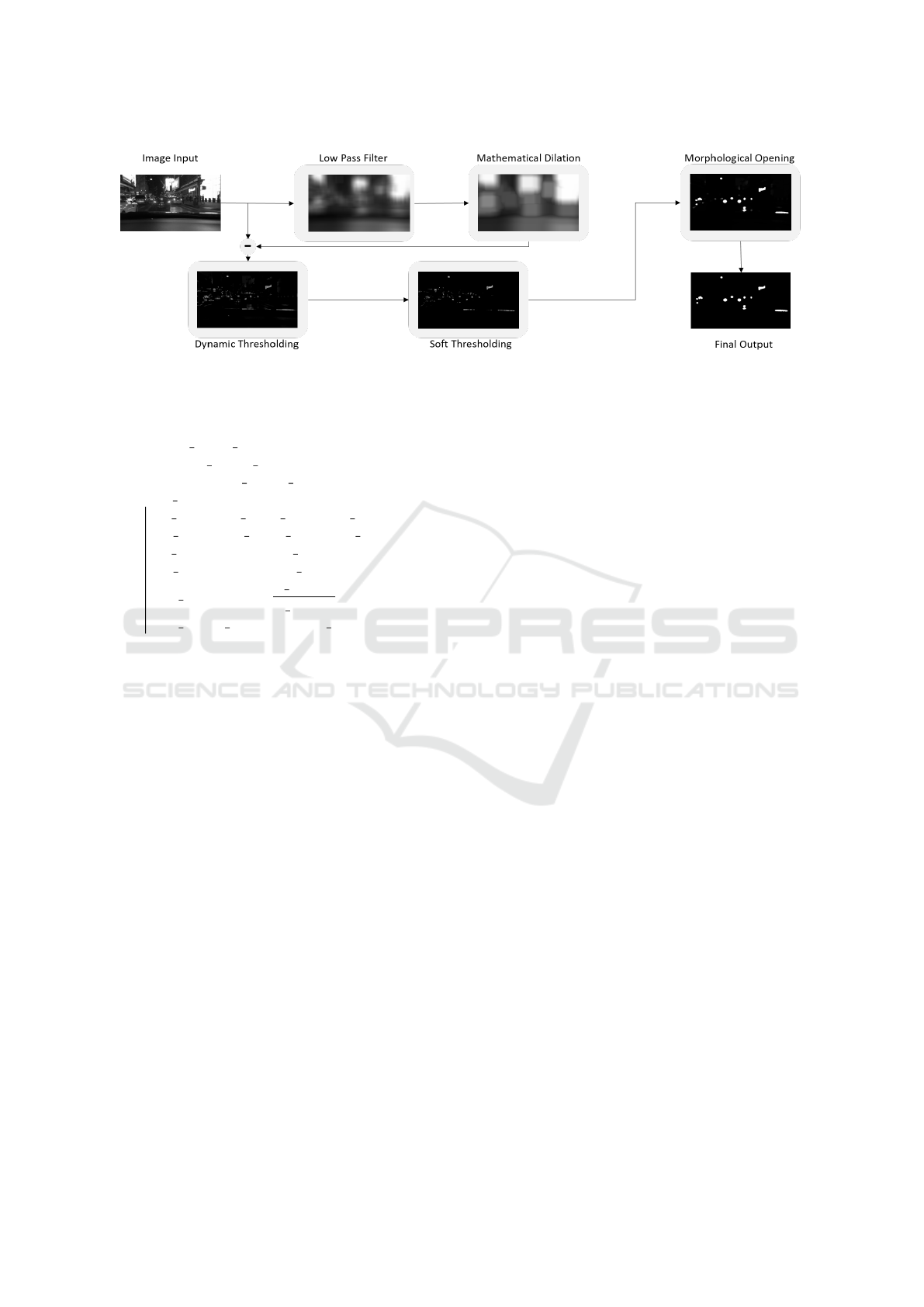
Figure 2: We employ light source detection derived from a highlight detection algorithm (Stojkovic et al., 2021) to generate
our nighttime dataset. This pipeline helps us locate each light source in the background image, resulting in more realistic
synthetic images.
Data: P list, N list, M
Result: llr curves list
initialization: llr curves list ← [ ];
for m inter in M do
P temp ← P list[P list.m ∈ m inter];
N temp ← N list[N list.m ∈ m inter];
P density ← KDE(P temp);
N density ← KDE(N temp);
llr temp ← log
10
P density
N density
;
llr curves list.append(llr temp);
end
Algorithm 1: Construction of Log-likelihood ratio curves
for different degrees of lens flare. These curves are derived
from the positives and negatives, which can tell the real dis-
tribution of the positives and negatives for different degrees
of lens flare according to a
k
.
4 EXPERIMENTAL EVALUATION
Due to the lack of datasets containing lots of lens
flare, we first synthesize a large-scale dataset of au-
tonomous driving scenarios with lots of lens flare
based on existing lens flare datasets and autonomous
driving datasets. Experimental and analysis are then
conducted on this synthesized dataset.
4.1 Datasets
We use two kinds of datasets, one is the autonomous
driving dataset and another is lens flare dataset:
4.1.1 Autonomous Driving Datasets
Many autonomous driving datasets exist, such as
BDD100K (Yu et al., 2020), nuScenes (Caesar et al.,
2020), etc. We opted for the BDD100K dataset due
to certain object annotations in the nuScenes dataset
being unobservable in image view, given its use of
multiple sensors. Additionally, the nuScenes dataset
comprises fewer scenes compared to the extensive
BDD100K dataset. BDD100K is solely annotated
based on images and offers a diverse, large-scale col-
lection of visual driving scenes, encompassing a wide
range of tasks.
4.1.2 Lens Flare Datasets
To generate an autonomous driving dataset with lens
flare, we use autonomous driving images as back-
ground images, and overlay images containing only
lens flare, without any background, onto these au-
tonomous driving background images. We use the
Flare7K (Dai et al., 2022) dataset as the nighttime lens
flare and used the dataset in paper (Wu et al., 2021)
as the daytime lens flare. The first dataset contains
light sources with different colors and sizes, consist-
ing of glare, shimmer, and streak, which are typical
lens flares that occur at nighttime. The second dataset
only contains the strong white light source, and it is
mainly used to simulate the sun’s lens flare in the day-
time.
The determination of daytime or nighttime can be
derived by quantifying the number of pixels below
a predefined threshold. For the daytime, we simply
add the one lens flare image to the brightest part of
the background image. However, in the nighttime,
we need to add more than one lens flare to the back-
ground image because normally there are more light
sources and the lens flare of a single light source is
smaller than that in daytime. Besides, it is helpful
to construct more accurate LLR curves by enlarging
the number of objects that are affected by lens flare.
Figure 2 illustrates how we find the location of light
sources in the nighttime images, we modify a high
light detection algorithm from paper (Stojkovic et al.,
VISAPP 2024 - 19th International Conference on Computer Vision Theory and Applications
344

2021) to achieve this, and then we can add one lens
flare to each detected light source.
4.2 Experiment Details
In the BDD100K dataset, the number of training,
validation, and test images are 70,000, 10,000, and
20,000 respectively. We first use the BDD100K train-
ing set without added lens flare to train the YOLOv5
middle-size (YOLOv5m) model to get a pre-trained
model for later use. Then we generate the images
with added lens flare. We apply the method men-
tioned in section 4.1 to the BDD100K validation set
and two lens flare datasets. It is worth noting that the
maximum number of added lens flares in one night-
time background image is 6 since the image will be-
come very unrealistic if we add too much lens flare to
it. Therefore, we have 10,000 images with lens flare.
The following experiments are all conducted based on
the synthetic dataset.
As we possess both synthetic images and their cor-
responding background images, we can compute the
Mean Square Error (MSE) for identical cropped de-
tected object images within them. The MSE value as-
sociated with each detected object can be interpreted
as the intensity of lens flare. A value of 0 indicates
no lens flare, while a higher MSE value indicates a
more severe lens flare on the detected object. Fig-
ure 3 gives some object examples with different MSE
values, providing a more intuitive visual sense of the
levels of lens flare represented by different MSE val-
ues. In this paper, we consider 0 < MSE ≤ 5000 as
very light lens flare, 5000 < MSE ≤ 10000 as light
lens flare, 10000 < MSE ≤ 15000 as moderate lens
flare, and MSE > 15000 as severe lens flare.
To demonstrate the effectiveness of our algo-
rithm, we must partition the 10,000 images from the
BDD100K validation set into two subsets: one for
constructing LLR curves (referred to as the ’training
subset’ in the subsequent sections of this paper) and
another for validation (referred to as the ’validation
subset’). To ensure a balanced distribution between
the training and validation subsets, we directly split
the output of YOLOv5m based on the MSE value of
each detected object at the object level rather than
the image level. For each degree of lens flare, we
randomly divided all detected objects into a training
subset and a validation subset, with 90% used for
constructing the LLR curves, and the remaining 10%
used for evaluating.
Figure 3: This image shows some object examples with dif-
ferent MSE values, providing a more intuitive visual sense
of the levels of lens flare represented by MSE values.
4.3 Result
We run a 10-fold cross-validation to get the final re-
sult. The threshold of Intersection over Union (IOU),
which is calculated as the ratio of the area of intersec-
tion between the predicted and ground truth bounding
boxes to the area of their union area and is often used
to determine whether a detected object is considered
a true positive or not, is set as 0.5.
In each validation iteration, we set the threshold
for different intensities of lens flare, for example, if
we set a threshold of lens flare metric as severe lens
flare, we include all detected objects affected by at
least severe lens flare, and sample 150 FP and TP
objects that are affected by less severe lens flare to
calculate the average precision (AP). We repeat this
sampling process 10 times for each threshold in each
validation iteration. From the figure 5, which is the
AP only for cars, the red line is always above the blue
line. The result shows that the proposed algorithm can
achieve better results in all experiment cases than the
original output of the YOLOv5m detector, especially
for those objects with more severe lens flare. In the
situation of no lens flare in figure 5, which means we
calculate AP across all detected objects, the improve-
ment is only about 0.1%. However, as the severity of
lens flare increases, the improvement becomes more
significant. When we consider a very severe lens flare,
the improvement reaches as high as 1.5%.
As depicted in Figure 5, a slight increase in AP
can be observed as the lens flare’s intensity reaches
its maximum in our experiment. We have investi-
gated this phenomenon and identified the main rea-
son: when the intensity of lens flare rises, the count of
objects significantly affected by severe lens flare di-
minishes, and most detected objects in this part have
low confidence scores and are background. Conse-
quently, the detected objects with very severe lens
flare are easier to classify as background at an earlier
stage of computing AP.
Although some classes in the BDD100K valida-
tion set only have limited instances, for classes with
sufficient instances to construct LLR curves and per-
form validation, the outcomes resemble those of cars.
We also adopt an alternative approach to assess the
Lens Flare-Aware Detector in Autonomous Driving
345

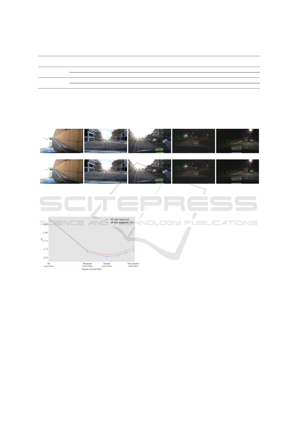
Table 1: AP for classes in BDD100K.
Degree of
Lens Flare
Methods Traffic light Vehicles
2
Traffic sign All classes
3
Moderate
Lens Flare
Fixed LLR 0.700±0.026 0.642±0.008 0.695±0.042 0.625±0.015
Adaptive LLR 0.723±0.022 0.646±0.008 0.698±0.043 0.634±0.015
Severe
Lens Flare
Fixed LLR 0.759±0.022 0.593±0.022 0.731±0.055 0.599±0.020
Adaptive LLR 0.784±0.021 0.601±0.017 0.740±0.054 0.614±0.020
1
We calculate results based on the threshold of lens flare metric as moderate and severe lens flare and run 100 times validations
on different sampled subsets respectively.
2
We grouped vehicles (car, truck, bus, train, motorcycle, and bicycle) into one category to calculate AP, due to limited instances
for certain classes in the BDD100K validation dataset.
3
The AP for all classes is calculated by treating all classes in the BDD100K dataset as a single class. The determination of TP and
FP is still based on individual classes. The unification into a single category is only considered during the LLR construction and
AP calculation.
(a)
(b)
Figure 4: Visual comparison on the validation subset (the threshold of lens flare metric is set as severe lens flare, only for cars)
by using a) adaptive LLR, b) fixed LLR. The green and blue rectangle is TP and FP respectively. Some cars are not detected
because they are used as the training subset to construct the LLR curves.
Figure 5: AP on cars for different degrees of lens flare.
From this chart, it can be observed that our method is more
effective as the lens flare becomes stronger.
proposed method on all classes in the BDD100K, as
depicted in Table 1. These results are obtained by
considering the situation of moderate and severe lens
flare and the same setting as before.
When treating all object classes as a single cate-
gory and computing one AP, we still achieve compa-
rable results. It should be noted that the determination
of TP and FP is still based on individual classes. The
unification into a single class is only considered dur-
ing the LLR construction and AP calculation.
The result of the Traffic light in Table 1 demon-
strates a more pronounced improvement facilitated by
our proposed method compared to those observed in
the case of cars. This is because when we synthe-
size images with lens flare, we add lens flare based
on the position of the light source. Therefore, traffic
lights are more significantly affected. The source of
variance here is due to the fact that we performed val-
idation and calculated averages across 100 different
sampled subsets. It’s worth noting that among all our
subsets, the results using adaptive LLR consistently
outperformed the fixed LLR. For instance, in the case
of the ”traffic light” category, when the AP based on
adaptive LLR reaches its lowest value, which is 0.70,
the corresponding AP using fixed LLR is only 0.67.
All the results in the table follow this pattern, demon-
strating the consistent effectiveness of our proposed
method.
Figure 4 gives us a visual comparison of the val-
idation subset (only cars) between the output of our
proposed method (figure 4a) and that of the original
YOLOv5m (figure 4b). The green and blue rectan-
gle is TP and FP respectively. Some cars are not de-
tected because they are sampled as the training subset
to construct the LLR curves. These results are gener-
ated by setting a threshold on precision on the training
subset, which is a common requirement in a practical
VISAPP 2024 - 19th International Conference on Computer Vision Theory and Applications
346

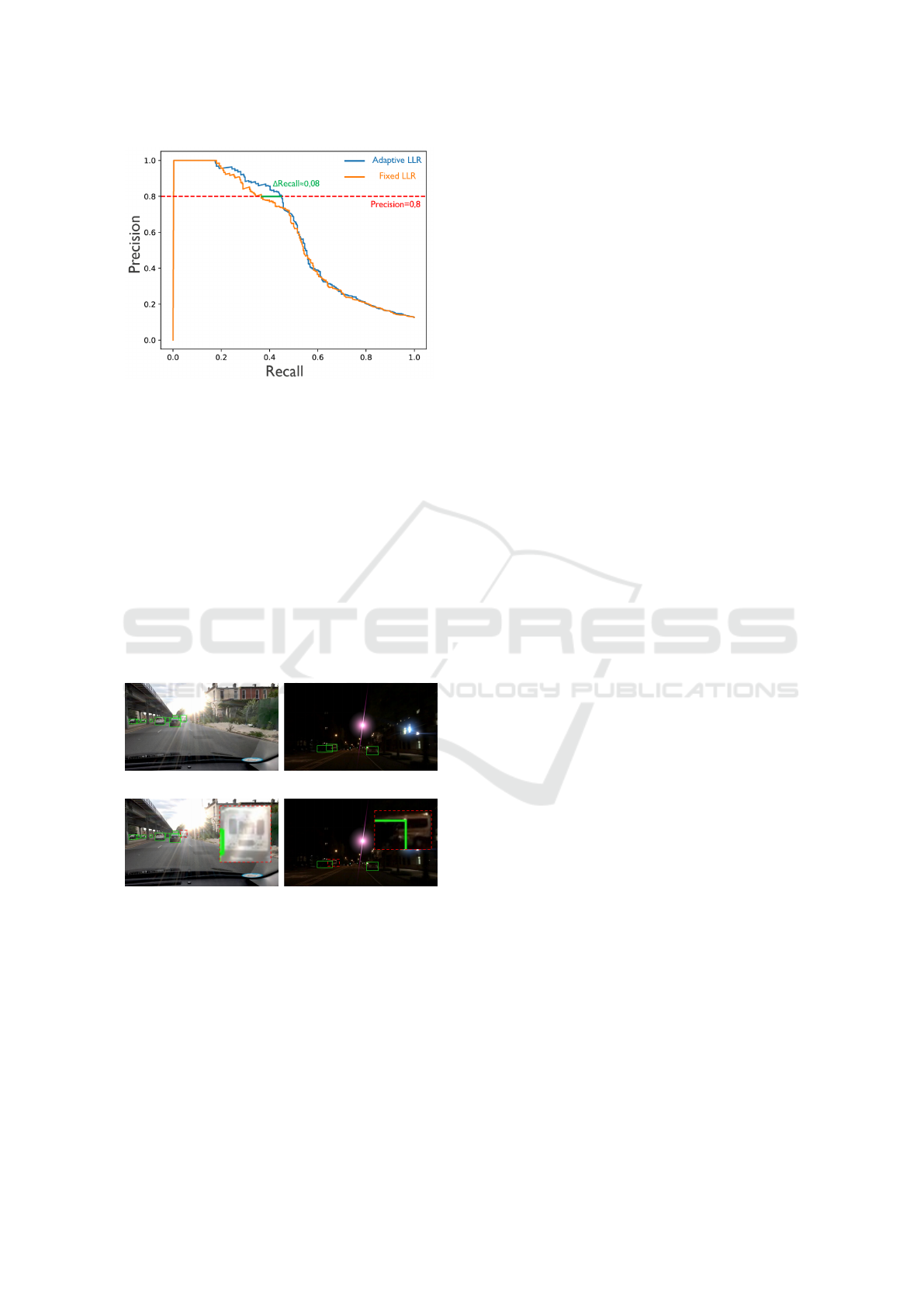
Figure 6: PR curves on cars for severe lens flare. In a practi-
cal autonomous driving task, we need to set a threshold for
the final output. Here we set a threshold on precision as 0.8.
Our proposed method can achieve a higher recall.
autonomous driving task, and then using this corre-
sponding LLR threshold to the output of detected ob-
jects in the validation subset to get the final decision
of positive and negative detections. Here we set the
threshold on precision as 0.8 and we conduct our ex-
periment on the validation subset by setting the lens
flare metric as severe lens flare. The results of our
proposed methods give more TPs without adding ex-
tra FPs than the original output of the YOLOv5m de-
tector. The result in figure 6 also shows that our pro-
posed method can achieve a higher recall when given
the same precision.
(a)
(b)
Figure 7: Detection results by using a) adaptive LLR, b)
fixed LLR. These images are not in the training and the val-
idation set. The red dashed rectangles are zoomed-in object
images.
Figure 7 is the detection result for images that are
not in the training and the validation set. We use the
entire BDD100K validation set to construct the LLR
curves and get a threshold of fixed and adaptive LLR
respectively for a given threshold on precision similar
to figure 6. Our method can still detect more objects
without adding additional FP objects.
5 CONCLUSION
In this paper, we proposed a lens flare-aware detec-
tor, which shows an improvement in object detection
in the presence of lens flare in autonomous driving
tasks, especially for those scenarios with severe lens
flare. Since our algorithm is based on the output of
the existing detector, it is easy to be deployed on top
of other object detectors.
We presented a study based on synthetic lens
flares, to allow for ground truth comparison. The syn-
thetic data experiments allowed us to directly measure
the lens-flare-induced difference in pixel value and
use them as a metric for lens flare severity (reference-
based). Further research should focus on deriving
such lens flare severity measures in a no-reference
scenario.
ACKNOWLEDGEMENTS
This work was supported by the Flemish Government
(AI Research Program).
REFERENCES
Caesar, H., Bankiti, V., Lang, A. H., Vora, S., Liong, V. E.,
Xu, Q., Krishnan, A., Pan, Y., Baldan, G., and Bei-
jbom, O. (2020). nuScenes: A multimodal dataset for
autonomous driving. In Proceedings of the IEEE/CVF
Conference on Computer Vision and Pattern Recogni-
tion, pages 11621–11631.
Chen, W.-T., Huang, Z.-K., Tsai, C.-C., Yang, H.-H., Ding,
J.-J., and Kuo, S.-Y. (2022). Learning multiple ad-
verse weather removal via two-stage knowledge learn-
ing and multi-contrastive regularization: Toward a
unified model. In Proceedings of the IEEE/CVF Con-
ference on Computer Vision and Pattern Recognition,
pages 17653–17662.
Crayton, T. J. and Meier, B. M. (2017). Autonomous Vehi-
cles: Developing a Public Health Research Agenda to
Frame the Future of Transportation Policy. Journal of
Transport & Health, 6:245–252.
Dai, Y., Li, C., Zhou, S., Feng, R., and Loy, C. C. (2022).
Flare7K: A phenomenological nighttime flare removal
dataset. In Thirty-sixth Conference on Neural Infor-
mation Processing Systems Datasets and Benchmarks
Track.
Dimitrievski, Martin (2023). Cooperative sensor fusion for
autonomous driving. PhD thesis, Ghent University.
Dosovitskiy, A., Beyer, L., Kolesnikov, A., Weissenborn,
D., Zhai, X., Unterthiner, T., Dehghani, M., Minderer,
M., Heigold, G., Gelly, S., et al. (2020). An image is
worth 16x16 words: Transformers for image recogni-
tion at scale. arXiv preprint arXiv:2010.11929.
Lens Flare-Aware Detector in Autonomous Driving
347

Girshick, R. (2015). Fast R-CNN. In Proceedings of the
IEEE International Conference on Computer Vision,
pages 1440–1448.
Group, I. W. et al. (2018). IEEE P2020 Automotive Imaging
White Paper.
Hnewa, M. and Radha, H. (2020). Object Detection Un-
der Rainy Conditions for Autonomous Vehicles: A
Review of State-of-the-Art and Emerging Techniques.
IEEE Signal Processing Magazine, 38(1):53–67.
Jocher, G., Chaurasia, A., Stoken, A., Borovec, J., Kwon,
Y., Michael, K., Fang, J., Yifu, Z., Wong, C., Montes,
D., et al. (2022). ultralytics/yolov5: v7. 0-YOLOv5
SOTA Realtime Instance Segmentation. Zenodo.
Liu, W., Anguelov, D., Erhan, D., Szegedy, C., Reed, S.,
Fu, C.-Y., and Berg, A. C. (2016). SSD: Single shot
multibox detector. In Computer Vision–ECCV 2016:
14th European Conference, Amsterdam, The Nether-
lands, October 11–14, 2016, Proceedings, Part I 14,
pages 21–37. Springer.
Liu, W., Ren, G., Yu, R., Guo, S., Zhu, J., and Zhang,
L. (2022). Image-adaptive YOLO for object detec-
tion in adverse weather conditions. In Proceedings
of the AAAI Conference on Artificial Intelligence, vol-
ume 36, pages 1792–1800.
Rashed, H., Ramzy, M., Vaquero, V., El Sallab, A., Sistu,
G., and Yogamani, S. (2019). Fusemodnet: Real-time
camera and lidar based moving object detection for ro-
bust low-light autonomous driving. In Proceedings of
the IEEE/CVF International Conference on Computer
Vision Workshops, pages 0–0.
Redmon, J., Divvala, S., Girshick, R., and Farhadi, A.
(2016). You only look once: Unified, real-time ob-
ject detection. In Proceedings of the IEEE Conference
on Computer Cision and Pattern Recognition, pages
779–788.
Ren, S., He, K., Girshick, R., and Sun, J. (2015). Faster R-
CNN: Towards Real-Time Object Detection with Re-
gion Proposal Networks. Advances in neural informa-
tion processing systems, 28.
Singh, S. (2015). Critical Reasons for Crashes Investigated
in the National Motor Vehicle Crash Causation Sur-
vey. Technical report.
Stojkovic, A., Aelterman, J., Luong, H., Van Parys, H.,
and Philips, W. (2021). Highlights Analysis System
(HAnS) for Low Dynamic Range to High Dynamic
Range Conversion of Cinematic Low Dynamic Range
Content. IEEE Access, 9:43938–43969.
Talvala, E.-V., Adams, A., Horowitz, M., and Levoy,
M. (2007). Veiling Glare in High Dynamic Range
Imaging. ACM Transactions on Graphics (TOG),
26(3):37–es.
Wu, Y., He, Q., Xue, T., Garg, R., Chen, J., Veeraragha-
van, A., and Barron, J. T. (2021). How to train neu-
ral networks for flare removal. In Proceedings of the
IEEE/CVF International Conference on Computer Vi-
sion, pages 2239–2247.
Yu, B., Chen, Y., Cao, S.-Y., Shen, H.-L., and Li, J. (2022).
Three-Channel Infrared Imaging for Object Detection
in Haze. IEEE Transactions on Instrumentation and
Measurement, 71:1–13.
Yu, F., Chen, H., Wang, X., Xian, W., Chen, Y., Liu, F.,
Madhavan, V., and Darrell, T. (2020). BDD100K:
A diverse driving dataset for heterogeneous multitask
learning. In Proceedings of the IEEE/CVF Conference
on Computer Vision and Pattern Recognition, pages
2636–2645.
VISAPP 2024 - 19th International Conference on Computer Vision Theory and Applications
348