Automatic Detection and Classiﬁcation of Atmospherical Fronts

Andreea Alina Ploscar

, Anca Ioana Muscalagiu

, Eduard Timotei Pauliuc

and Adriana Mihaela Coroiu

Department of Computer Science, Babes

-Bolyai University, M. Koganiceanu 1 Street, Cluj-Napoca, Romania

Keywords:

Atmospherical Fronts, Detection, Classiﬁcation, Convolutional Neural Network.

Abstract:

This paper presents an application that uses Convolutional Neural Networks (CNN) for the automatic detection

and classiﬁcation of atmospherical fronts in synoptic maps, which are a graphical representation of weather

conditions over a speciﬁc geographic area at a given point in time. These fronts are signiﬁcant indicators of

meteorological characteristics and are essential for weather forecasting. The proposed method takes in a region

extracted from a synoptic map to detect and classify fronts as cold, warm, or mixed, setting our study apart

from existing literature. Furthermore, unlike previous research that typically utilizes atmospheric data grids,

our study employs synoptic maps as input data. Additionally, our model produces a single output, accurately

representing the front type with a 78% accuracy rate. The CNN model was trained on data collected from

various meteorological stations worldwide between 2013 and 2022. The proposed tool can provide valuable

information to weather forecasters and improve their accuracy.

1 INTRODUCTION

The atmospheric front (or air front) represents the

transition between two air masses different in den-

sity or temperature. Their contact can cause radical

weather changes, such as precipitation, temperature,

or pressure variations. The difference in temperature

between the two air groups that an atmospheric front

separates determines what kind of front it is. Cold

fronts, warm fronts, and occluded fronts are the three

major types of atmospheric fronts. Apart from these

types, there exists an additional category, stationary

fronts, which have similar characteristics to occluded

fronts, having in common the mix of warm and cold

air masses. For the purpose of this study, we will

consider both occluded and stationary fronts as mixed

air fronts. The type of the front is determined by the

dominating type of air mass: cold or warm. When a

cold air mass approaches a warm air mass, the warm

air mass is forced to ascend quickly, creating a cold

front. Warm air rises, cools, condenses, and forms

clouds and precipitation as a consequence of conden-

sation. When a warm air mass approaches a cold air

mass, the warm air gently rises over the denser, colder

https://orcid.org/0009-0009-6021-3538

https://orcid.org/0009-0000-3139-4311

https://orcid.org/0009-0007-7450-0824

https://orcid.org/0000-0001-5275-3432

air. This is known as a warm front. As a conse-

quence, a wide band of clouds and light precipitation

are formed. When a chilly front passes by, it becomes

obscured.

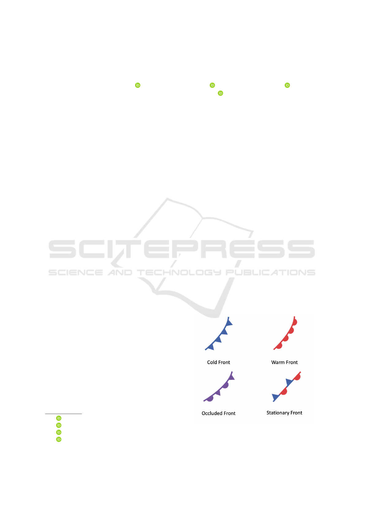
In synoptic-type weather maps (Bergeron, 1980),

the two air masses are delimited by continuous lines,

and the type of air front is determined by different ge-

ometric shapes: semicircles for warm fronts, triangles

for cold fronts, and alternating triangles and semicir-

cles for mixed fronts.

Figure 1: Types of Fronts.

Ploscar, A., Muscalagiu, A., Pauliuc, E. and Coroiu, A.

Automatic Detection and Classiﬁcation of Atmospherical Fronts.

DOI: 10.5220/0012306700003636

Paper published under CC license (CC BY-NC-ND 4.0)

In Proceedings of the 16th International Conference on Agents and Artiﬁcial Intelligence (ICAART 2024) - Volume 3, pages 94-100

ISBN: 978-989-758-680-4; ISSN: 2184-433X

Accurate detection of atmospheric fronts holds

signiﬁcant importance for meteorologists and weather

forecasters as it enables precise weather predictions

and timely warnings. By monitoring these fronts,

forecasters can anticipate weather patterns and effec-

tively communicate potential hazards like thunder-

storms, blizzards, or ﬂoods to the public. In our study,

the primary research question revolves around the

possibility of classifying atmospheric fronts within a

smaller area (less than 350,000 sq km) using a CNN

with an accuracy exceeding 60%.

This paper aims to use Convolutional Neuronal

Networks on synoptic maps collected from meteoro-

logical stations to determine in an automatic manner

the existence and category of fronts over the territory

of a country in a speciﬁc moment. Automatic front

detection is a subject addressed very little in the past

years (Niebler et al., 2022) (Matsuoka et al., 2019),

and only for broader territories like Europe and Amer-

ica.

In this paper we propose an intelligent algorithm

for solving the problem of determining and classify-

ing atmospherical fronts, using Convolutional Neural

Networks. The study aims to provide an intuitive,

easy-to-use, and user-friendly tool for specialists in

the meteorological ﬁeld that will consist aid in fore-

casting different weather characteristics on smaller

regions, such as the territory of a country. To our

knowledge, there have been no studies of the auto-

matic classiﬁcation of fronts using synoptic maps as

input, therefore the model proposed in this paper aims

to serve as a starting point for further research on front

detection and classiﬁcation in synoptic maps.

The present work is structured in ﬁve chapters as

follows. The ﬁrst chapter is an introduction to the

problem of air front detection and its meteorologi-

cal importance. Next, the following chapter presents

the current state of the art in this domain, illustrat-

ing a short comparison between the existing papers

and our approach. In the third chapter, we outline

our comprehensive approach, including a detailed ac-

count of our methodology, the dataset collected, the

pre-processing steps undertaken, the network archi-

tecture of our Convolutional Neural Network (CNN),

the training process, as well as an explanation of

the metrics used to evaluate the performance of our

model. Moving on to the fourth chapter, we present

the results of our experiments, highlighting both the

strengths and weaknesses of our model. Finally, we

provide a summary of our ﬁndings, outline the limi-

tations of our model, and discuss potential ideas for

further improvements.

2 LITERATURE REVIEW

The detection and classiﬁcation of air fronts are usu-

ally addressed manually, but the demand for an au-

tomatic approach increased along with the dataset

volume. The detection and classiﬁcation of weather

fronts using deep learning models is a scarcely ex-

plored ﬁeld, having only a few published papers in

recent years.

We are presenting two related works that utilize

deep neural networks to detect and classify weather

fronts. The ﬁrst work ’S. Niebler et al.: Automatic

detection and classiﬁcation of fronts, 2022’ (Niebler

et al., 2022) focuses on detecting and classifying ﬁve

types of fronts (warm front, cold front, occlusion, sta-

tionary front or background) over a large area using

multi-level ERA5 reanalysis data, atmospherical data

grids. The second work is (Matsuoka et al., 2019)

’Daisuke Matsuoka et al.: Automatic detection of sta-

tionary fronts around Japan using a deep convolu-

tional neural network, 2019’ that detects only station-

ary fronts in a smaller area around Japan using GPV-

MSM mesoscale numerical prediction data.

In paper (Niebler et al., 2022) the authors intro-

duced a deep neural network (U-Net) to detect and

classify ﬁve types of fronts using atmospheric data

grids provided by ERA5, ECMWF. The input data is

represented as a two-dimensional matrix, where each

cell corresponds to a speciﬁc location and time, con-

taining weather parameters. The method used is a

CNN that automatically learns atmospheric features

that correspond to the existence of a weather front.

For each spatial grid point, the algorithm predicts a

probability distribution, the likelihood of the point be-

longing to one of the ﬁve classes. The validation is

done through the critical success index (CSI), prob-

ability of object detection (POD), and success rate

(SR). The model obtains prediction scores with a crit-

ical success index higher than 66.9% and an object

detection rate of more than 77.3%. Frontal climatolo-

gies of the network are highly correlated (greater than

77.2%) to climatologies created from weather service

data.

Moreover, Daisuke Matsuoka proposed a U-Net

convolutional neural network that detects only sta-

tionary fronts around Japan (Matsuoka et al., 2019).

The input data are weather data with multiple chan-

nels, and the output front data is a polyline that is

compared with the polylines extracted from label data

to optimize the model. The detection performance

is evaluated by calculating the similarity between the

prediction result and the ground truth based on the

Tanimoto coefﬁcient. The paper does not specify an

exact estimate of the accuracy, but it provides a vi-

Automatic Detection and Classiﬁcation of Atmospherical Fronts

sual comparison of the ground truth and the detected

fronts. The model succeeded in extracting the approx-

imate shape of seasonal rain fronts, such as the Baiu

front and autumnal rain front, but its performance de-

creased upon the approach of a typhoon.

In comparison with these papers, our study fo-

cuses on an arbitrary area, with an approximate size

of an average country. Thus, the output of our algo-

rithm contains a single result, one of the four classes.

Another important distinction is the type of input our

algorithm uses, the synoptic maps, in comparison to

atmospherical data grids, which is an entirely differ-

ent meteorological map representations. As a ﬁnal

distinction, our model is able to classify all 3 types

of fronts on a particular area, not only discovering the

existence of a particular one in a certain territory.

3 METHODOLOGY

The research plan chosen for this project requires

a methodology that adopts both theoretical analysis

and practical design, achieved through implementa-

tion and experimentation with different CNN models

and datasets.

3.1 Dataset

The input data of the problem is represented by sets

of ”synoptic map” type images, collected from dif-

ferent weather stations, in which different meteoro-

logical characteristics are represented: air pressure,

temperature and humidity, baric tendency, wind di-

rection and speed. Thus, the model aims to detect the

air fronts over a small chosen territory from the initial

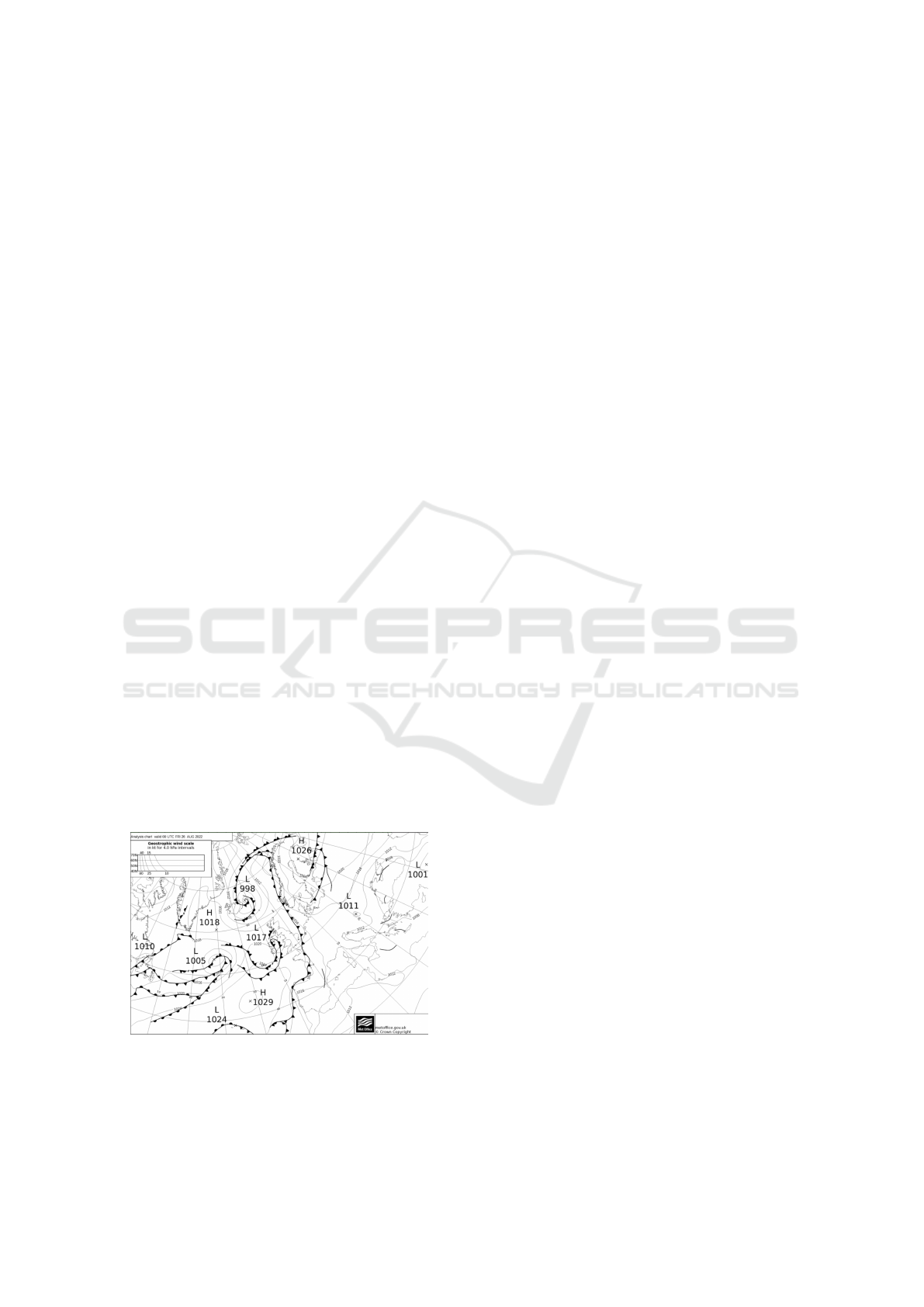
synoptic map. The format of the map is presented in

2. The study uses synoptic map datasets, downloaded

Figure 2: Synoptic Map.

from Wetterzentrale (wet, ), a German weather ser-

vice that provides synoptic maps daily. The data was

manually collected by the authors, obtaining roughly

650 synoptic maps from different years and seasons

between 2013-2022.

3.2 Input Preprocessing

The approach in this paper involves a few steps of

preprocessing of the input data. The initial images

received from the weather stations cover the Europe

continent, containing multiple or even all types of

fronts, making the result of the classiﬁcation mean-

ingless. To obtain input data that can be classiﬁed

under a predominant class, the synoptic maps were

divided into 9 equally sized tiles. This method low-

ers the chance of an image containing multiple fronts,

as it covers a smaller area. The tiles were manually

labelled into one of the 4 categories (no front, cold

front, warm front or mixed front) by the most predom-

inant one, if there were multiple present in the picture.

To generate more data, we augmented the data by ro-

tating the tiles with 90, 180 respectively 270 degrees,

thus generating another 3 front lines with different di-

rections. Using this method, we gathered roughly 160

pictures per class from which 25% were used for val-

idation purposes.

To avoid overﬁtting to one class, we have used

equally sized datasets from each category for the

training and validation data. In order to increase the

performance of our CNN in real life situations we

have used both simple, easily identiﬁable fronts and

more complex pictures illustrating multiple types of

fronts, having a predominant one. This makes our

datasets more realistic and relevant.

3.3 Network Architecture

The algorithm used is based on the classical model for

image recognition through supervised learning, mak-

ing use of Convolution Neural Networks with multi-

ple convolution, pooling and dropout layers.

Convolutional Neural Networks (CNNs) are a type

of neural network that is commonly used in image

and video recognition tasks. CNNs are speciﬁcally

designed to effectively handle spatial input data, such

as images, by leveraging a series of convolutional lay-

ers (O’Shea and Nash, 2015). A CNN consists of

multiple layers, including convolutional layers, pool-

ing layers, and fully connected layers. The input to

a CNN is a tensor, typically representing an image,

which is passed through a series of convolutional lay-

ers. Each convolutional layer consists of a set of ﬁlters

that are convolved with the input tensor to produce a

set of output features.

The ﬁlters used in the convolutional layers are

learned during the training process, allowing the net-

ICAART 2024 - 16th International Conference on Agents and Artiﬁcial Intelligence

work to learn features that are speciﬁc to the input

data. These learned features are then used to classify

the input data.

Pooling layers are used to downsample the output

features from the convolutional layers, reducing the

spatial dimensions of the data while preserving the

most important information. This helps to reduce the

number of parameters in the network, making it more

efﬁcient to train.

Finally, the output from the last pooling layer is

passed through a series of fully connected layers,

which perform classiﬁcation on the features extracted

by the convolutional and pooling layers.

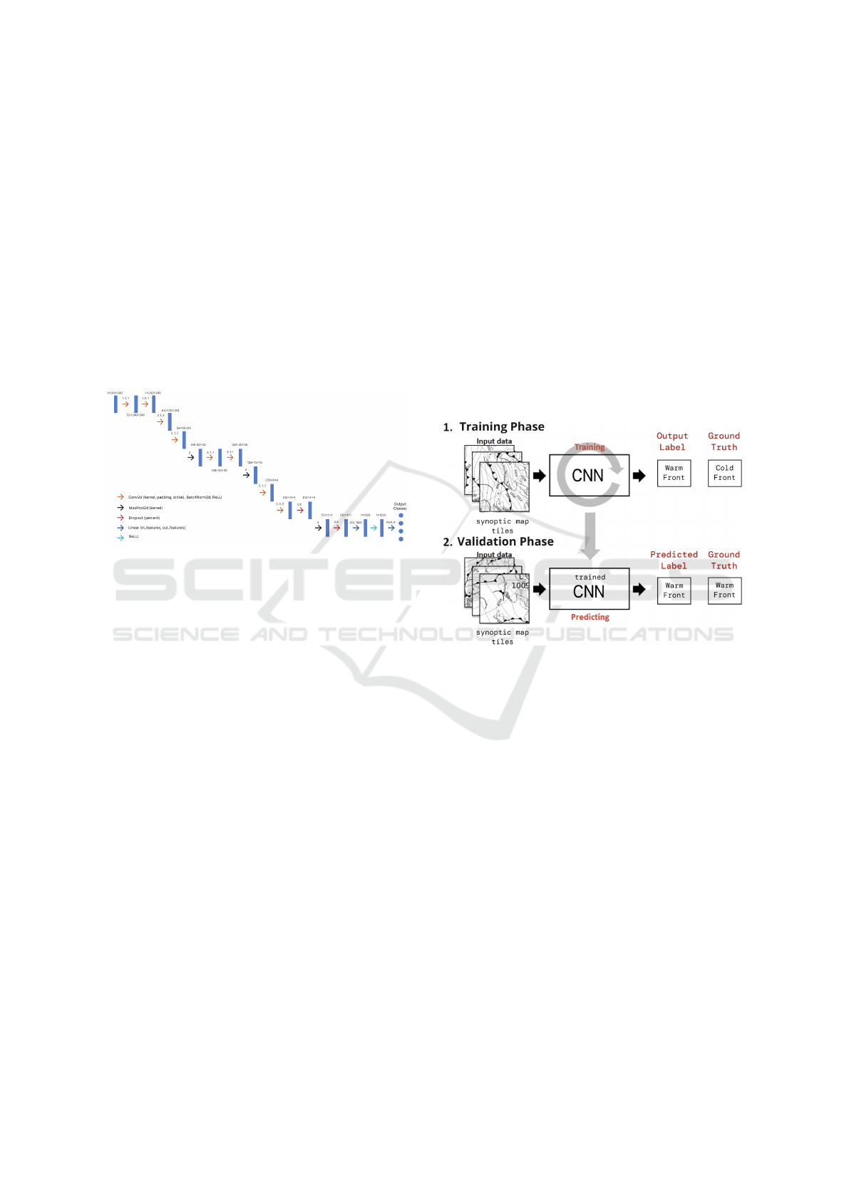
The CNN architecture used in our paper is de-

picted in 3.

Figure 3: CNN model.

Our CNN model starts with images of a minimum

size of 240x240, as they are all adjusted to this reso-

lution before entering the ﬁrst layer. The model is or-

ganized in multiple 2D convolution layers, taking into

consideration the format of the input image (black and

white) which is represented with only one slice, aver-

age pooling, and dropout layers, which help prevent

overﬁtting. The last step of the neural network is the

ﬂattening phase, outputting the probability of the in-

put belonging to each of the 4 classes. For the ﬁrst

layer, the number of input channels is 1 because the

algorithm uses black-and-white images. After the 2D

convolution is applied, the layer performs, in addi-

tion, a batch normalization and a rectiﬁed linear unit

function (ReLU). All of the convolutional and pooling

layers form the sequential layer, which is followed by

the ﬂattening phase.

3.4 Training Process

The phases of the Training and Validation process are

presented in Figure 4.

Our experiments start with loading the data, be-

ing split into train and validation data. These two are

shufﬂed into batches of 32 images, in order to max-

imize the probability of having each type of front in

all batches to acquire knowledge about all fronts after

processing each batch.

The training phase starts with no accuracy, slightly

increasing over the epochs. In each epoch, the algo-

rithm trains the model and iterates over batches of im-

ages loaded from the training dataset. The classes are

predicted using images from the current batch and the

output is compared to the actual labels. The loss func-

tion used is cross entropy and it backpropagates the

loss into the network. This allows the parameters to

be adjusted according to the computed gradients.

After the iteration, the learning rate is adjusted,

decreasing with the current epoch. The train loss and

accuracy are measured using the predictions and the

actual labels for all images from each batch. The val-

idation phase evaluates the model on the correspond-

ing dataset and saves the model if greater accuracy is

obtained.

Figure 4: Conceptual Diagram of Training and Validation

Process.

3.5 Metrics and Performance

Assessment

In order to evaluate our method we are measuring the

number of correctly classiﬁed fronts, computing the

overall and by class accuracy. We also compute a con-

fusion matrix to better visualize the performance of

our CNN model. We display this matrix as a heatmap

and we plot the evolution with each epoch of the over-

all and by class accuracy.

A Confusion Matrix for multiple classes is a ma-

trix that summarizes the performance of a machine

learning model by comparing the predicted class la-

bels with the actual class labels. It is a valuable tool

for evaluating the performance of a model and can be

used to calculate various metrics to assess its effec-

tiveness.

In our case, the confusion matrix is a square grid

having the number of rows equal to the number of

Automatic Detection and Classiﬁcation of Atmospherical Fronts

classes. Each row in the confusion matrix represents

the instances in a predicted class, while each column

represents the instances in an actual class. The value

in each cell (i,j) of the matrix represents the percent-

age of instances that were classiﬁed as i but actually

belonged to j. Therefore, our aim is to have the largest

percentages on the main diagonal, which represents

the percentage of correctly classiﬁed instances.

Accuracy is a measure of how well a predictive

model is able to correctly predict the outcome or class

label of a given input. Formally, accuracy is deﬁned

as the ratio of the number of correctly predicted in-

stances to the total number of instances in the dataset.

In multi-class classiﬁcation problems, where there are

more than two possible classes, the number of in-

stances that were correctly classiﬁed as each class

needs to be counted separately. The accuracy for

multi-class classiﬁcation is then calculated as:

Accuracy =

correct classi f ications

all classi f ications

(1)

Therefore, in order to monitor the accuracy of our

model after learning in each epoch, we are plotting

the evolution of our accuracy during training.

This paper tests the hypothesis that atmospheric

fronts covering a small area ( less than 350000 sq km)

can be classiﬁed by a CNN with an accuracy of over

60%. For each epoch, we measure the training loss

and train and validation accuracy. If the validation

accuracy is better than the best accuracy measured so

far we save the model and upgrade the best one. We

train the model over 100 epochs, saving intermediary

best models.

In comparison with other articles, because the aim

of our experiment was classiﬁcation and not detection

of the fronts as in (Niebler et al., 2022), we were able

to measure the performance of our algorithm numeri-

cally, as described above, through the number of cor-

rectly classiﬁed pictures, making use of all the clas-

sic performance assessment methods used in the ML

ﬁeld.

4 RESULTS AND DISCUSSIONS

This study involved conducting experiments using

two models with different architectures, which will be

detailed in the following sections. These sections will

compare the training datasets, architectures, and re-

sults obtained from the experiments. It is worth men-

tioning that the second approach demonstrates a no-

table improvement resulting from modiﬁcations made

to the model structure and enhancements in the data

quality utilized in our study.

4.1 Initial Version

To better understand the problem and the input data

we started experimenting with a model similar to the

one developed in paper (Niebler et al., 2022), having

a simpliﬁed U-Net architecture in order to suit our

smaller images better. We observed that the model

shows lower performance on our data. The architec-

ture can be observed in Figure 5 and the results of

the validation data can be observed in Figure 6. The

dataset used for the ﬁrst experiment contains ≈ 300

images.

Figure 5: CNN Model Version 1.

By analyzing the results obtained we noticed that

the model can easily detect the presence of a front but

classifying the type of front has a lower performance.

Figure 6: Confusion matrix Version 1.

4.2 Final Version

The ﬁrst improvement brought to the model focuses

on enhancing the training and validation datasets by

adding more input data and improving its quality, both

by using higher resolution images and ﬁltering out

images that were too hard to classify usually because

more than one front could be identiﬁed. The archi-

tecture of the model is also improved, with a new ap-

proach that can be visualized in Figure 3.

The best model we obtained during the training

phase had an accuracy of 78% and was saved after the

ICAART 2024 - 16th International Conference on Agents and Artiﬁcial Intelligence

20th epoch. We provide the accuracy overall and the

accuracy per class evolution in Figure 7 and Figure 8.

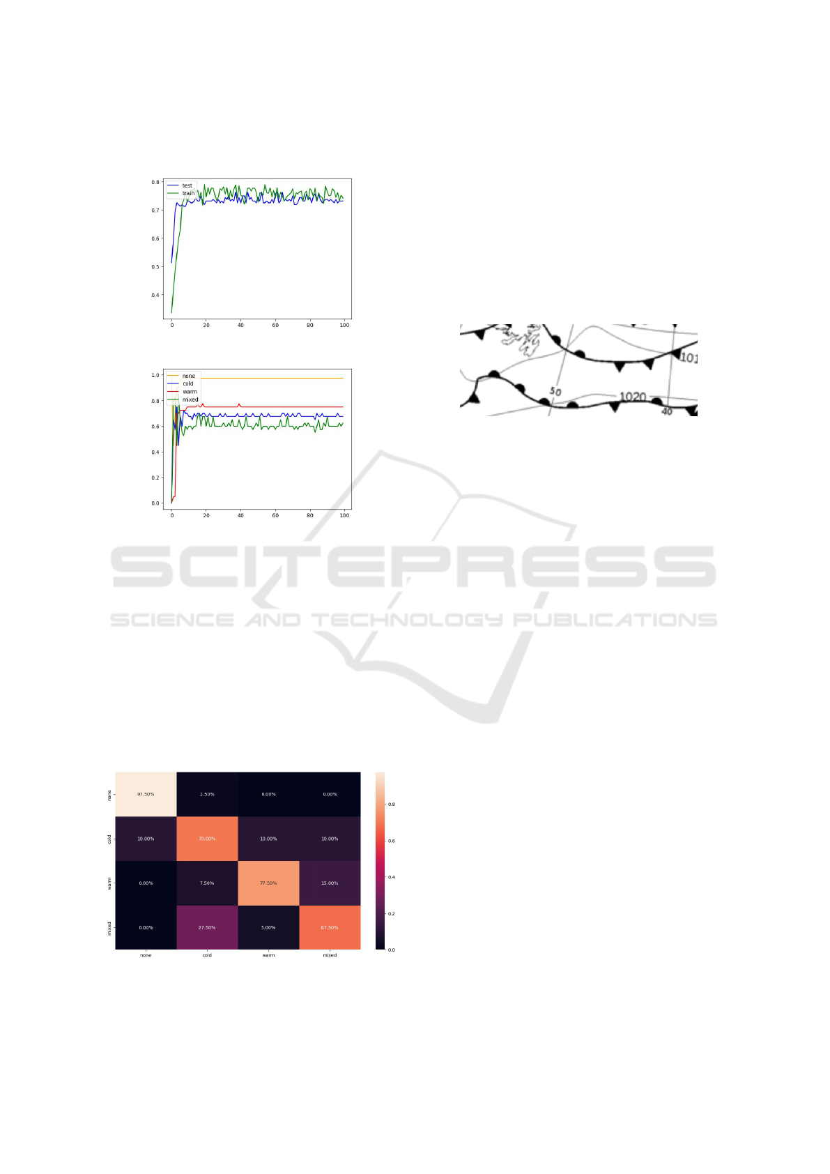
Figure 7: Train and Validation Accuracy.

Figure 8: Accuracy Per Class Evolution.

It is noticeable that in the overall accuracy plot,

our model learns the most in the ﬁrst 20 epochs of the

training, converging towards an accuracy of 78% in

the following epochs. The oscillation of the accuracy

in the ﬁrst epochs is present due to the encountering

of a new class in the processed batch of the current

epoch. In the accuracy per class plot, it is evident that

our model demonstrates proﬁcient performance in de-

tecting the presence of a front and a similar accuracy

in detecting cold, warm, and mixed fronts.

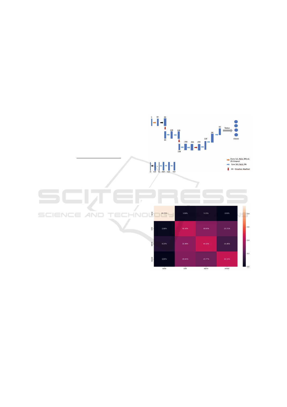
A more reﬁned overview of the performance is

provided by the confusion matrix described in Figure

9, obtained by plotting it as a heatmap.

Figure 9: Confusion matrix.

It can be observed that the model’s biggest ﬂaw

is its tendency to misidentify cold fronts as mixed

fronts, with a 27.5% error rate. This issue arises be-

cause of the quality of our data, some of the syn-

optic map tiles contain both warm and cold fronts (

with cold fronts being the predominant ones ) and our

model may mistake a tile with a cold and a warm front

with a mixed one. The difference between the two

cases consists of the fact that the two polylines of the

fronts may overlap and create the illusion of a mixed

front, as can be observed in Figure 10.

Figure 10: Cold and Warm Fronts Alternatively.

5 CONCLUSIONS AND FURTHER

WORK

The main conclusion that can be drawn is that Auto-

matic Front Detection can be a very efﬁcient solution

for the issues we currently face in weather prediction.

Our study demonstrates that a supervised learning

model, even with a relatively small training dataset,

can accurately classify the types of fronts present on

a small area from a synoptic map. One of the most

important strengths of our approach is that our exper-

iment paves the path for further research and for the

discovery of new approaches in the domain, which is

currently very little represented in the research world.

Considering that, to our knowledge, this research is

one of the ﬁrst to approach front classiﬁcation on

small areas, we have encountered a few shortcomings

in our experiments. One of the most relevant weak-

nesses to our approach is the training dataset, which

is very hard to obtain and label because they are not

publicly available in larger sets. In addition to this, the

synoptic maps might not be consistent in the future,

depending on how meteorologists decide to represent

the fronts.

There is deﬁnitely room for improvement in the

model developed, as it is one of the ﬁrst to approach

this issue. Two possible directions that could increase

the performance are larger, more qualitative training

datasets and more efﬁcient processors that could sup-

port more epochs of training.

Automatic Detection and Classiﬁcation of Atmospherical Fronts

ACKNOWLEDGEMENTS

The realization of this work was made possible with

the support of our dedicated professors, to whom we

would like to express our gratitude: Professor, Ph.D.

Laura Silvia Dios

an (Babes

-Bolyai University, Com-

puter Science Department) and to Assoc. Professor,

Ph.D. Adina Eliza Croitoru (Babes

-Bolyai University,

Faculty of Geography).

REFERENCES

https://www.wetterzentrale.de. Online; accessed 15 June,

2023.

Bergeron, T. (1980). Synoptic meteorology: an historical

review. Pure and Applied geophysics, 119(3):443–

473.

Matsuoka, D., Sugimoto, S., Nakagawa, Y., Kawahara, S.,

Araki, F., Onoue, Y., Iiyama, M., and Koyamada,

K. (2019). Automatic detection of stationary fronts

around japan using a deep convolutional neural net-

work. SOLA, 15:154–159.

Niebler, S., Miltenberger, A., Schmidt, B., and Spichtinger,

P. (2022). Automated detection and classiﬁcation

of synoptic-scale fronts from atmospheric data grids.

Weather and Climate Dynamics, 3(1):113–137.

O’Shea, K. and Nash, R. (2015). An introduction

to convolutional neural networks. arXiv preprint

arXiv:1511.08458.

ICAART 2024 - 16th International Conference on Agents and Artiﬁcial Intelligence

100