Anomaly Detection Methods for Finding Technosignatures
Rohan Loveland and Ryan Sime
Dept. of Electrical Eng. and Computer Science, South Dakota School of Mines and Technology, Rapid City, SD, U.S.A.
Keywords:
Anomaly Detection, Rare Category Detection, Variational Autoencoders, Technosignatures, Lunar,
Spacecraft.
Abstract:
Machine learning based anomaly detection methods are used to find technosignatures, in this case human
activity on the Moon, in high resolution imagery for four anomaly detection methods: autoencoder based
reconstruction loss, kernel density estimate of probability density, isolation forests, and the Farpoint algorithm.
A deep learning variational autoencoder was used which provided both a reconstruction capability as well
as a means of dimensionality reduction. The resulting lower dimension latent space data was used for the
probability density and isolation forest methods. For our data, we use Lunar Reconnaissance Orbiter high
resolution imagery on four known mission locations, with large areas broken into smaller tiles. We rank
the tiles by anomalousness and determine the gains in efficiency that would result from showing the tiles in
that order as compared to using random selection. The resulting efficiency in reduction of necessary amount
of analyst time ranges into factors in the hundreds depending on the particular mission, with the Farpoint
algorithm generally having the best performance. We also combine the tiles into bounding boxes based on
spatial proximity, and demonstrate that this could provide a further improvement in reduction efficiency.
1 INTRODUCTION
Machine learning based anomaly detection methods
have been developed and applied to a variety of ap-
plications, ranging from intrusion detection to medi-
cal applications to energy consumption (Nassif et al.,
2021). In this effort, we apply anomaly detection to
the problem of finding technosignatures, which can
be defined as evidence of past or present usage or di-
rect presence of technology. Here we approach this
by looking for technosignatures on the Moon in lunar
imagery (with the expectation that these will be from
human activity). Thus, technosignatures in this case
range from crashed probe remnants to rover tracks.
The Lunar Reconnaissance Orbiter (LRO) has
been deployed in orbit around the moon to acquire
high resolution imagery, which allows for the possi-
bility of finding crashed probes and other extant tech-
nosignatures. We examine four missions in particular
with known locations and widely differing character-
istics (e.g. crewed landings and crashes).
We select imagery in large regions containing
the four missions, and divide these regions into
tiles, designating the small subset of tiles that con-
tain technosignatures (”TSig tiles”). We apply four
anomaly detection methods: autoencoder reconstruc-
tion loss, kernel density estimated probabilities, iso-
CVZ
Figure 1: Lunar imagery at a variety of resolutions, with the
smallest scale from imagery captured by LRO, showing the
Ranger 6 crash site crater.
lation forests, and the Farpoint algorithm. Each of the
methods provides us with a ranking of the tiles from
least to most anomalous, and we compare the rela-
tive efficiency in terms of which method would most
rapidly find the TSig tiles.
2 RELATED WORK
Extensive research has been conducted in the field
of anomaly detection, with surveys in (Xu et al.,
2019),(Ruff et al., 2021). A number of Deep Learn-
ing (DL) based methods have been investigated, with
a survey in (Pang et al., 2021).
Loveland, R. and Sime, R.
Anomaly Detection Methods for Finding Technosignatures.
DOI: 10.5220/0012306400003654
Paper published under CC license (CC BY-NC-ND 4.0)
In Proceedings of the 13th International Conference on Pattern Recognition Applications and Methods (ICPRAM 2024), pages 633-640
ISBN: 978-989-758-684-2; ISSN: 2184-4313
Proceedings Copyright © 2024 by SCITEPRESS – Science and Technology Publications, Lda.
633

In the area of anomaly detection applied to im-
agery, four standard methods for anomaly detection
are described in detail in (Yang et al., 2021): den-
sity estimation, image reconstruction, one-class clas-
sification, and self-supervised classification. A num-
ber of the methods have been developed particularly
for analyzing medical imagery; a survey of DL based
methods is available in (Alloqmani et al., 2021). Ref.
(Zhang et al., 2020) applied DL Anomaly Detection
methods to finding Covid-19 in lung imagery with
good results.
The density estimation techniques rely on the fact
that data points that are considered to be anomalous
should have a correspondingly low probability den-
sity. These techniques generally have some kind of
scale parameter, e.g. ’bandwidth’ in kernel density es-
timation (Rosenblatt, 1956). Isolation Forests bypass
this by normalizing the results with expected values
from binary search trees (Liu et al., 2008), and can
still be used for density estimation, smoothed over the
results from an ensemble of trees.
A different approach is based on using reconstruc-
tion error from DL autoencoders (Zhou and Paffen-
roth, 2017). The idea in this case is that the encoders
are constrained to have small enough latent spaces
so that they can only do a good job reconstructing
”normal” points, and correspondingly less on those
that are anomalous. The basic autoencoders were ex-
tended in (Kingma and Welling, 2013) to ”Variational
Auto Encoders” (VAE’s), which constrained the latent
space representation to a multi-variate normal distri-
bution. These were further extended to a Gaussian
Mixture Model in (Zong et al., 2018).
The previous approaches are based on viewing
anomaly detection as a binary classification problem,
in some cases by finding an ”anomalousness mea-
sure” that allows ranking the points and then applying
a threshold to separate the ’anomalous’ from the ’nor-
mal’ points. A different approach is to view anomaly
detection as a multi-class problem, where allowance
for different kinds of anomalies are made (Loveland
and Amdahl, 2019).
Machine learning methods have been applied for
analyzing lunar data in a number of respects, with,
e.g. (Kodikara and McHenry, 2020) classifying lu-
nar soils. As our ability to see further into space
and deploy probes with higher resolution sensors in-
creases, more emphasis is being placed on detect-
ing technosignatures (Haqq-Misra et al., 2022). Ref.
(Lesnikowski et al., 2020) uses LRO imagery to look
for technosignatures, but limits their approach to bi-
nary classification using VAE’s.
3 DATA
NASA’s LRO was launched in 2009 and has been or-
biting the Moon since at an altitude of 50-200 km,
making up to 4 passes per day (NASA, 2023a). Its
instrumentation includes two Narrow Angle Cameras
(NACs) that are designed to provide 0.5 meter-scale
panchromatic images over a 5 km swath. The re-
sulting high resolution data is available from NASA’s
Planetary Data System archive (NASA, 2023b).
Some examples of lunar imagery are shown in Fig.
1.
A table of anthropogenic impacts and space-
craft on the moon has been compiled at (Williams,
2023). This lists the dates, landing types, locations (if
known), and statuses of whether or not the landing site
has been imaged for over 70 spacecraft. Other sources
of information are also available, e.g. (Wagner et al.,
2017). All of these human activities left technosigna-
tures that can be used to evaluate anomaly detection
algorithm performance. For this research, we selected
four different missions:
• Ranger 6 - Crash Landing;
• Apollo 12 - Crewed Landing with Rover;
• Apollo 13 - Crash Landing - Large Profile;
• Apollo 17 - Crewed Landing - Low Light.
For each of these missions, we extracted ”region” im-
ages which contained the mission area as well as a sig-
nificant amount of the surrounding lunar surface. The
region images were broken into tiles of 64x64 pix-
els/side, overlapping with a stride of 32 pixels (both
vertically and horizontally). Each of these tiles was
then flattened into a vector in a 4,096 dimensional fea-
ture space.
The indexes of the tiles containing evidence of the
spacecraft (technosignature or ”TSig” tiles) were then
identified and stored for performance evaluation. The
region sizes varied slightly, but contained approxi-
mately 18,000,000 pixels, corresponding to approx-
imately 17,000 tiles, with 4 TSig tiles for Ranger 6,
44 for Apollo 12 (the larger number is due to rover
track tiles), 9 for Apollo 13, and 4 for Apollo 17. Ex-
ample TSig tiles for each mission are shown in Fig. 2,
in pseudo-color.
Figure 2: Positive technosignature tiles for each mission.
ICPRAM 2024 - 13th International Conference on Pattern Recognition Applications and Methods
634

4 METHODS
We approach the problem of detection of technosig-
natures in two different ways:
• as a standard anomaly detection problem, in
which binary classification is used with the data
partitioned into an ”anomaly” class and a ”normal
class”.
• as a rare class detection problem within an imbal-
anced dataset where one or more majority classes
dominate, and a number of different anomaly
classes may exist.
The former leads to a ”tiles-only” approach, in which
individual tiles are just presented in an order deter-
mined by their anomalousness score.
The latter suggests that tiles that are from the same
class should be grouped together, particularly if they
are spatially close. This leads to the ”bounding box”
approach, where tiles that are close are grouped to-
gether and presented to the user as a single instance.
Results from both of these approaches are presented
below.
Beyond the form of what is presented to a user, a
number of different methods can be used to determine
anomalousness and/or membership in a rare class. We
examine: a random baseline, deep autoencoders, deep
variational autoencoders, isolation forests, and an un-
supervised Farpoint implementation. Several of these
methods can be used to produce an ”anomalousness”
score directly, which can then be ranked and pre-
sented in order. Each of these is discussed in more
detail below.
4.1 Random Baseline
The performance of a random baseline algorithm can
be calculated in terms of the expected values of the
numbers of tiles that would have to be queried in order
to find the TSig tiles.
The calculation is as follows: let N
be the total number of tiles, G = {tile g
i
:
g
i
contains a technosignature},G = |G | and B,b, and
B be defined similarly for the non-TSig tiles. Then
G + B = N (1)
For the tiles b
j
∈ B, define indicator functions I
j
such
that:
I
j
=
(
1, b
j
is queried before any tiles g
i
∈ G
0, otherwise
(2)
Then,
E[I
j
] =
1
G + 1
(3)
Let X
1
− 1 be the number of tiles queried before a tile
g
i
∈ G is found. Then
X
1
− 1 =
B
∑
j=1
I
j
(4)
Therefore,
E[X
1
] =
B
G + 1
+ 1 =
N + 1
G + 1
. (5)
This provides us with the expected value of the num-
ber of queries before the first TSig tile is drawn. This
can then be extended by ”starting over” with the N
′
remaining tiles, and G
′
remaining TS tiles. We can
re-use equation 5 to get
N
′
= N −
N + 1
G + 1
and G
′
= G − 1 (6)
and then find the expected value of the number of
queries to find the second TSig tile using
E[X
2
] = E[X
1
] +
N
′
+ 1
G
′
+ 1
(7)
Some algebra results in
N
′
+ 1
G
′
+ 1
=
N + 1
G + 1
so that E[X
n
] = nE[X
1
] (8)
4.2 Variational Auto Encoders
Deep autoencoders (AE’s) have been used as a
method for anomaly detection based on the idea that
they preferentially learn to encode ”normal” samples,
with correspondingly poor reconstruction for anoma-
lous ones (Zhou and Paffenroth, 2017).
This is achieved by forcing the neural network to
have a low dimensional ”bottleneck” in between the
encoder and decoder. This represents a latent space
which has significantly lower dimensionality than the
input and output (which have the same dimensional-
ity). An anomalousness score for each input can be
calculated using the autoencoder based on the mean
squared error of the reconstruction loss. An exten-
sion of the autoencoder, the ”variational autoencoder”
(VAE), where the probability density of the latent
space is shaped to be a multi-variate normal density,
was proposed to improve performance (Kingma and
Welling, 2013).
We compared the performance of AE’s to VAE’s
and concluded that the VAE’s had generally better
performance. We also compared a number of differ-
ent dimensionalities for the latent space and ended up
selecting 64 dimensions as providing the best perfor-
mance.
The two primary differences in implementation
between AE’s and VAE’s are the addition of random
Anomaly Detection Methods for Finding Technosignatures
635

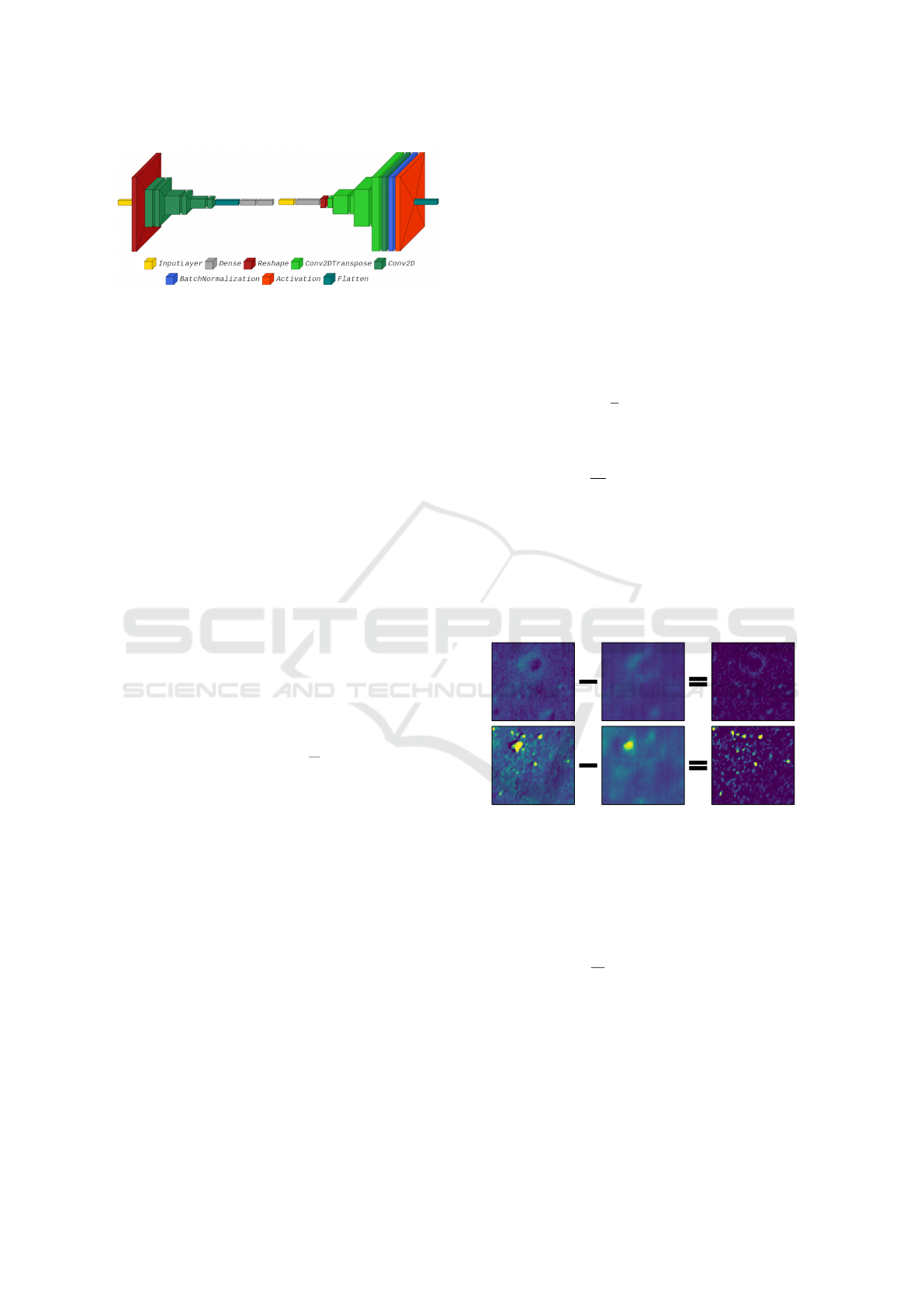
Figure 3: The variational autoencoder model architecture.
sampling to the latent space term and a modification
of the loss function. These are described briefly be-
low, along with the specific neural net architectures
shown in Fig.3.
4.2.1 Encoder Network
The inputs for the encoder are the tile vectors re-
shaped into 64x64x1 tensors. The encoder has three
pairs of convolution layers: the first layer of each pair
uses 3x3 kernels and strides of 2 with 32, 64, and 64
filters respectively. The second layer of each pair uses
1x1 kernels with strides of 1 and 16 filters each. For
every layer, the ReLU activation function is used. The
resulting 8x8x16 tensor is flattened and fed through
two parallel 64-node dense layers which represent the
means and variances of the VAE’s multi-variate nor-
mal distribution.
4.2.2 Sampler
The sampler adds random normal noise ε scaled by λ
= 0.05 to the mean. The resulting latent space z is:
z = µ + λεe
σ
2
2
(9)
which is based off of the implementation of (Chol-
let, 2021).
4.2.3 Decoder Network
The decoder feeds the latent space into a 1024-node
dense layer and reshapes it into an 8x8x16 tensor.
There are six layers that mirror the encoder layers:
convolution transposes with 16, 64, 16, 64, 16, and 32
filters respectively with the same kernels and strides
as their encoder counterparts. After the transposes,
a final convolution with 1 filter, a 1x1 kernel, and a
stride of 1 is applied to reduce the filter space. Batch
normalization and a sigmoid activation are applied be-
fore flattening the output to the original vector of size
4096.
4.2.4 Training
The model was trained with the Adam optimizer us-
ing a variety of batch sizes ranging from 32-512 over
a range of 50-250 epochs with the best results using
a batch size of 32 over 50 epochs. The total train-
ing loss for each epoch is the average of each batch’s
loss, which is the sum of the average binary cross-
entropy reconstruction loss and the Kullback-Leibler
divergence loss:
loss = loss
r
+ loss
KL
(10)
where
loss
r
=
1
S
S
∑
i=0
M−1
∑
j=0
BCE(x, r) (11)
and
loss
KL
= −
1
2S
L
∑
i=0
(1 + σ
2
i
− µ
2
i
− e
σ
2
i
) (12)
where BCE is the binary cross-entropy function, x and
r are the original and reconstructed images, S is the
batch size, M is the number of features in the tiles,
and µ
i
and σ
i
are the mean and standard deviation in
the latent space of dimensionality L such that {µ
i
,σ
i
:
i ∈ 1..L}.
Original Reconstruction Difference
Figure 4: Low α
RE
sample (top row) vs. High α
RE
sample
(bottom row).
4.2.5 Reconstruction Based Anomalousness
A measure of anomalousness based on reconstruction
error, α
RE
, is implemented with:
α
RE
=
1
M
M
∑
i=1
(I
rec
(i) − I
input
(i))
2
(13)
where I
rec
(i) and I
input
(i) are the intensity values of
the flattened versions of the reconstructed and input
images at location i, and M is the total number of pix-
els. Graphically, this is illustrated for two tiles in Fig.
4.
A histogram of α
RE
, with the top 100 anomalies,
is shown in Fig. 5. A bimodal distribution would
ICPRAM 2024 - 13th International Conference on Pattern Recognition Applications and Methods
636

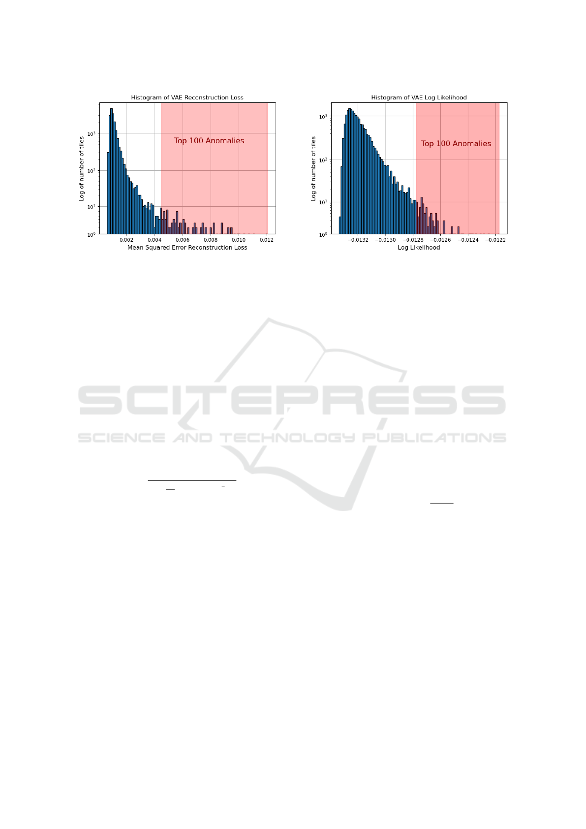
Figure 5: α
RE
scores for Ranger 6 tiles encoded into the
latent space of dimensionality L=64.
support a division between a ’normal’ population and
anomalous classes. We do see a possible ’notch’
slightly to the left of the top 100 region which may
be indicative of this, but we do not investigate this
further here.
4.2.6 Likelihood Based Anomalousness
The previous section described a measure of anoma-
lousness based on the reconstruction loss of the VAE.
An alternative method is to view anomalies as sam-
ples falling in low probability density areas. An esti-
mate of this underlying density from the latent space
representation z can be obtained using kernel density
estimation, which we modify to obtain an anomalous-
ness measure of inverse log likelihood, α
LLk
, using:
α
LLk
=
1
log(
1
hN
∑
N
i=1
e
−1/2(
z
h
)
2
)
(14)
where h is the bandwidth/smoothing parameter, and N
is the number of points. The bandwidth h is selected
as:
h = 10 ∗ max({σ
i
: i ∈ 1..L}) (15)
where σ
i
is the standard deviation of the VAE in the
i
th
dimension in the latent space of dimensionality L.
A histogram of α
LLk
, with the top 100 anomalies,
is shown in Fig. 6. We note the presence of a possi-
ble ’notch’ separating ’normal’ and anomalous popu-
lations here as well.
4.2.7 Dimensionality Reduction
Beyond the previously described anomalousness
measures, the VAE can be used for dimensionality re-
duction since it produces a lower dimensional latent
space after the encoder. Experimentation over a range
of latent space dimensionalities showed that the per-
formance of the VAE anomalousness calculations, as
Figure 6: α
LLk
scores for Ranger 6 based on the density
estimates of the latent space.
well as that of the isolation forest, was best using a 64
dimensional latent space.
4.3 Isolation Forests
Isolation Forests were developed as a tree-based
anomaly detection technique based on the number of
randomly selected node divisions necessary to isolate
a given input sample (Liu et al., 2008). Averaging
these path lengths over a large number of individually
constructed trees allows for an ensemble estimate of
the probability density, which can then be used as an
estimate of anomalousness.
We used the sci-kit learn implementation on the
64-dimensional latent space data representation from
the VAE encoder. The corresponding anomalousness
score, which we designate as α
IF
for consistency, is
based on:
α
IF
= −1(0.5 − 2
−E(h(z))
c(N)
) (16)
where c(N) is the average search length for a dataset
of size N,
c(N) = 2 ln N − 1 + γ − 2(N − 1)/N (17)
where γ is Euler’s constant, approximately 0.577. We
insert a ’-1’ into equation 16 in order to make more
positive values indicate increasing anomalousness.
A histogram of α
IF
, with the top 100 anomalies,
is shown in Fig. 7. A case can be made for a ’notch’
here as well.
4.4 Farpoint Algorithm
The Farpoint algorithm is based on treating anomaly
detection as a rare class detection problem, rather than
strict binary classification or anomalousness scoring
(Loveland and Amdahl, 2019),(Loveland and Kaplan,
Anomaly Detection Methods for Finding Technosignatures
637

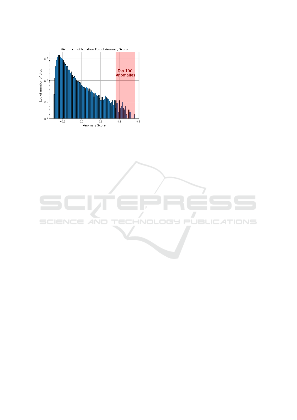
Figure 7: α
IF
scores for the original feature space of Ranger
6.
2022). It is normally used in a semi-supervised, active
mode, where samples are sequentially presented to an
oracle/user who is queried for a corresponding label.
The label is used by the algorithm to attempt to find a
sample from a different class each time, in the process
minimizing the overall number of queries required to
find all classes. In this mode, Farpoint acts as both an
algorithm for rare class detection and as a classifier
for imbalanced datasets.
It is also possible to run Farpoint in an unsuper-
vised mode, circumventing the oracle by providing
every point with a different label. This was the mode
used here, because the tiles contained a mixture of
classes and we lacked the domain expertise to pro-
vide proper labels for everything except TSig tiles.
In this mode it is clear that no meaningful classifier
will result, but the order in which the tiles are pre-
sented can be seen as a ranking for anomalousness.
The results of using both the original 4,096 dimen-
sional input feature space and the reduced 64 dimen-
sional latent space were compared, with the algorithm
performing better on the full, unreduced, input.
5 RESULTS
We first present results for the tile-only approach, and
then results for tiles combined into bounding boxes.
5.1 Tiles
Standard classification metrics (e.g. precision, recall)
are not directly applicable here because a human ana-
lyst needs to be presented with only a single tile con-
taining a TSig to trigger a subsequent, larger scale
search. Therefore, we consider the number of queries
required to find the first positive occurrence to be the
salient measure. Expressing this relative to the ex-
pected results from a random strategy gives us ”First
Occurrence Efficiency” (FOE
M
) for method ”M”:
FOE
M
=
query # of first TSig using random selection
query # of first TSig using algorithm
(18)
The numerator is the expected value from the random
selection method, given by Eqn. 5, while the denom-
inator is dependent on the particular method chosen
(e.g. VAE Reconstruction Loss).
The results from the various spacecraft missions
are shown in Table 1. In general, the table shows that
these algorithms could reduce the amount of samples
that a human analyst might have to look at by factors
in the hundreds.
Farpoint has the best performance, followed by
isolation forests and then the VAE based techniques.
The large variation in performance between scenarios
is reflective of the differences in difficulty between
them; Apollo 17 scored much lower than the oth-
ers because it has a small profile, and can easily be
mistaken as just another large rock, while Apollo 13
TSigs were so distinct that they ranked as the most
anomalous tile by three of the four methods.
The number of queries that it takes to find the first
four occurrences for each of the missions are shown
in Fig. 8. The top two figures both show results
for Ranger 6 for two different tile offsets, with little
difference in number of queries to find the first oc-
currence, except for VAE Reconstruction Loss. Far-
point’s performance is best in 3 of the 4 scenarios for
finding the first TSig, but generally takes longer to
find the other occurrences after the first. This is to be
expected given that it attempts to present classes that
are different from any presented so far.
5.2 Bounding Boxes
Simply presenting tiles ranked by anomalousness
score is potentially less useful to a user than group-
ing data samples into classes. This is apparent here
where a large rock field might have a correspondingly
large number of anomalous tiles, none of which are
relevant. We partially address this by thresholding a
number of anomalous tiles (e.g. 50) and then find-
ing bounding boxes that include all 8-connected tile
neighbors. This has the potential to further reduce the
number of overall items that are separately presented
to a user. The bounding boxes resulting from Far-
point and Ranger 6 are shown in Fig. 9. In this case
the user would have only need to see seven bound-
ing boxes before finding Ranger 6, as opposed to 14
tiles, thereby saving a factor of 2. Similar or greater
reductions occur for the other scenarios.
ICPRAM 2024 - 13th International Conference on Pattern Recognition Applications and Methods
638

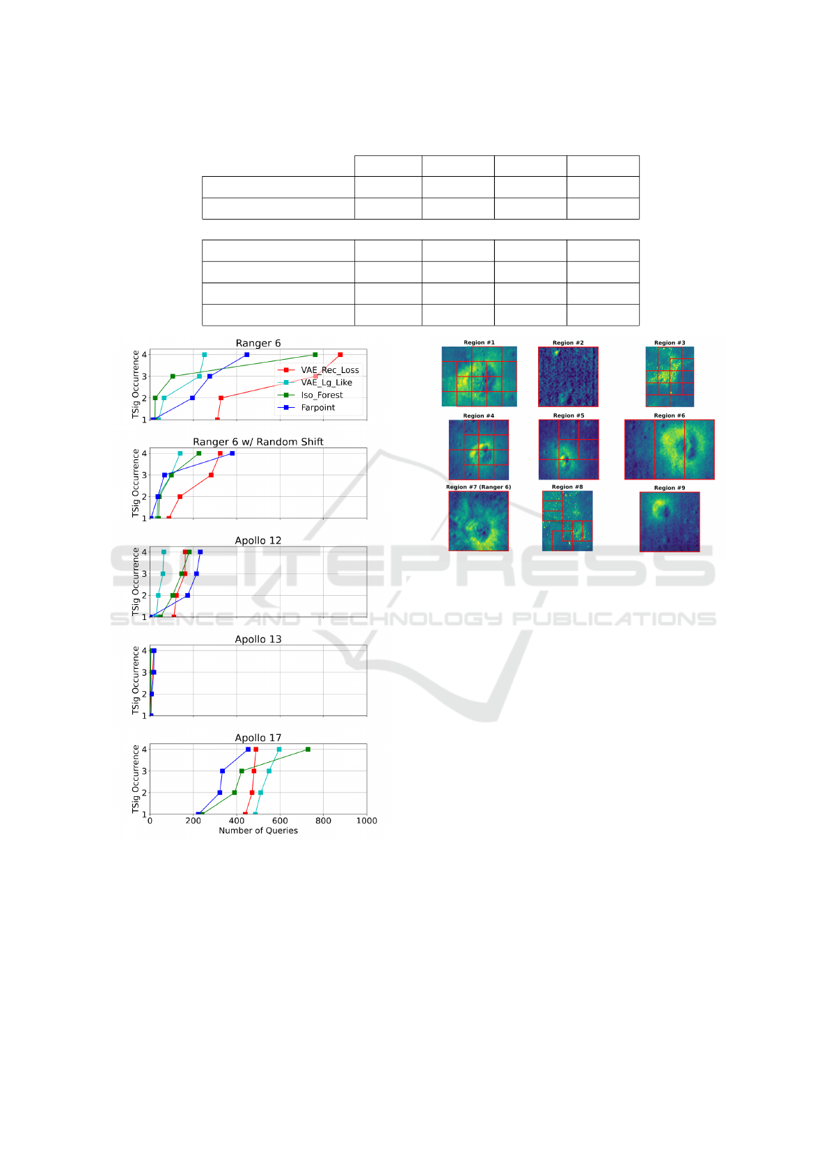
Table 1: Shows the first occurrence efficiency (FOE) for the spacecraft missions and differing methods.
Ranger 6 Apollo 12 Apollo 13 Apollo 17
# TSig Tiles
4 44 9 4
Random Selection
3422 380 1711 3422
First Occurrence Efficiencies
VAE Rec. Loss
11.0 3.4 1711.0 7.8
VAE 1/Log Likelihood
85.6 13.1 1711.0 7.0
Isolation Forest
148.8 7.8 1711.0 14.3
Farpoint (Unsupervised)
244.4 380.0 342.2 15.3
Figure 8: First four occurrences of technosignature tiles for
each spacecraft.
6 CONCLUSION
Applying machine learning based anomaly detection
methods to lunar imagery can significantly reduce the
amount of time required to find technosignatures, po-
tentially by factors ranging into the 100’s or more. Of
Figure 9: Bounding boxes and queried tiles corresponding
to the first 9 unique regions detected by Farpoint.
the methods used, Farpoint has generally better per-
formance than VAE based reconstruction loss, VAE
probability density, and isolation forests, even used in
it’s unsupervised mode.
Moving beyond the binary classification of
anomalies to a multi-class framework offers the po-
tential for even more gains in reduction efficiency, as
evidenced by the combination of anomalous tiles into
bounding boxes.
This effort has focused on using known mission
locations in order to allow for performance evalua-
tion, but the present work can easily be extended, with
input from an appropriate domain expert, to mount a
methodical search for lost probe locations. Part of this
process would ideally involve further algorithm de-
velopment to better address dealing with data at mas-
sive scale (e.g. imagery of the entire moon).
In the process of conducting that effort, it would
be desirable to curate the LRO imagery based on the
optimal solar incidence angles to only process images
with high contrast lighting. This is motivated by the
difficulty that each method had locating the Apollo 17
TSig tile compared to the other missions, which could
be attributed to the weak lighting of the imaged area
resulting in low contrast tiles.
Anomaly Detection Methods for Finding Technosignatures
639

Future work will also involve extending the exist-
ing algorithm to address the numerous applications in
streaming data in system health monitoring, cyberse-
curity, etc.
REFERENCES
Alloqmani, A., Abushark, Y. B., Khan, A. I., and Alsolami,
F. (2021). Deep learning based anomaly detection in
images: insights, challenges and recommendations.
International Journal of Advanced Computer Science
and Applications, 12(4).
Chollet, F. (2021). Deep learning with Python. Simon and
Schuster.
Haqq-Misra, J., Ashtari, R., Benford, J., Carroll-
Nellenback, J., D
¨
obler, N. A., Farah, W., Fauchez,
T. J., Gajjar, V., Grinspoon, D., Huggahalli, A., et al.
(2022). Opportunities for technosignature science in
the planetary science and astrobiology decadal survey.
arXiv preprint arXiv:2209.11685.
Kingma, D. P. and Welling, M. (2013). Auto-encoding vari-
ational bayes. arXiv preprint arXiv:1312.6114.
Kodikara, G. R. and McHenry, L. J. (2020). Machine learn-
ing approaches for classifying lunar soils. Icarus,
345:113719.
Lesnikowski, A., Bickel, V. T., and Angerhausen, D.
(2020). Unsupervised distribution learning for lu-
nar surface anomaly detection. arXiv preprint
arXiv:2001.04634.
Liu, F. T., Ting, K. M., and Zhou, Z.-H. (2008). Isolation
forest. In 2008 eighth ieee international conference
on data mining, pages 413–422. IEEE.
Loveland, R. and Amdahl, J. (2019). Far point algorithm:
active semi-supervised clustering for rare category de-
tection. In Proceedings of the 3rd International Con-
ference on Vision, Image and Signal Processing, pages
1–5.
Loveland, R. and Kaplan, N. (2022). Combining active
semi-supervised learning and rare category detection.
In Advances in Deep Learning, Artificial Intelligence
and Robotics, pages 217–229. Springer.
NASA (2023a). Lunar reconnaissance orbiter website. http
s://lunar.gsfc.nasa.gov/about.html.
NASA (2023b). Planetary data system archive website. ht
tps://pds.nasa.gov/.
Nassif, A. B., Talib, M. A., Nasir, Q., and Dakalbab, F. M.
(2021). Machine learning for anomaly detection: A
systematic review. Ieee Access, 9:78658–78700.
Pang, G., Shen, C., Cao, L., and Hengel, A. V. D. (2021).
Deep learning for anomaly detection: A review. ACM
computing surveys (CSUR), 54(2):1–38.
Rosenblatt, M. (1956). Remarks on some nonparametric
estimates of a density function. The annals of mathe-
matical statistics, pages 832–837.
Ruff, L., Kauffmann, J. R., Vandermeulen, R. A., Mon-
tavon, G., Samek, W., Kloft, M., Dietterich, T. G., and
M
¨
uller, K.-R. (2021). A unifying review of deep and
shallow anomaly detection. Proceedings of the IEEE,
109(5):756–795.
Wagner, R., Nelson, D., Plescia, J., Robinson, M., Speyerer,
E., and Mazarico, E. (2017). Coordinates of anthro-
pogenic features on the moon. Icarus, 283:92–103.
Williams, D. (2023). Table of anthropogenic impacts and
spacecraft on the moon. https://nssdc.gsfc.nasa.gov/
planetary/lunar/lunar artifact impacts.html.
Xu, X., Liu, H., Yao, M., et al. (2019). Recent progress of
anomaly detection. Complexity, 2019.
Yang, J., Xu, R., Qi, Z., and Shi, Y. (2021). Visual
anomaly detection for images: A survey. arXiv
preprint arXiv:2109.13157.
Zhang, J., Xie, Y., Li, Y., Shen, C., and Xia, Y. (2020).
Covid-19 screening on chest x-ray images using deep
learning based anomaly detection. arXiv preprint
arXiv:2003.12338, 27(10.48550).
Zhou, C. and Paffenroth, R. C. (2017). Anomaly detec-
tion with robust deep autoencoders. In Proceedings
of the 23rd ACM SIGKDD international conference
on knowledge discovery and data mining, pages 665–
674.
Zong, B., Song, Q., Min, M. R., Cheng, W., Lumezanu,
C., Cho, D., and Chen, H. (2018). Deep autoencoding
gaussian mixture model for unsupervised anomaly de-
tection. In International conference on learning rep-
resentations.
ICPRAM 2024 - 13th International Conference on Pattern Recognition Applications and Methods
640