Teeth Localization and Lesion Segmentation in CBCT Images

Using SpatialConﬁguration-Net and U-Net

Arnela Hadzic

, Barbara Kirnbauer

, Darko

Stern

and Martin Urschler

1 a

Institute for Medical Informatics, Statistics and Documentation, Medical University of Graz, Graz, Austria

Department of Dental Medicine and Oral Health, Medical University of Graz, Graz, Austria

Institute of Computer Graphics and Vision, Graz University of Technology, Graz, Austria

Keywords:

Teeth Localization, Lesion Segmentation, SpatialConﬁguration-Net, U-Net, CBCT, Class Imbalance.

Abstract:

The localization of teeth and segmentation of periapical lesions in cone-beam computed tomography (CBCT)

images are crucial tasks for clinical diagnosis and treatment planning, which are often time-consuming and re-

quire a high level of expertise. However, automating these tasks is challenging due to variations in shape, size,

and orientation of lesions, as well as similar topologies among teeth. Moreover, the small volumes occupied

by lesions in CBCT images pose a class imbalance problem that needs to be addressed. In this study, we pro-

pose a deep learning-based method utilizing two convolutional neural networks: the SpatialConﬁguration-Net

(SCN) and a modiﬁed version of the U-Net. The SCN accurately predicts the coordinates of all teeth present in

an image, enabling precise cropping of teeth volumes that are then fed into the U-Net which detects lesions via

segmentation. To address class imbalance, we compare the performance of three reweighting loss functions.

After evaluation on 144 CBCT images, our method achieves a 97.3% accuracy for teeth localization, along

with a promising sensitivity and speciﬁcity of 0.97 and 0.88, respectively, for subsequent lesion detection.

1 INTRODUCTION

Cone-beam computed tomography (CBCT) is a

highly effective medical imaging technique used to

generate a 3D image of the oral and maxillofacial re-

gion, with various applications in dentistry (Khana-

gar et al., 2021; Umer and Habib, 2022). However,

the analysis and documentation of CBCT images typ-

ically require a signiﬁcant amount of time and exper-

tise from professionals. While automated methods

have been proposed to localize and segment anatomi-

cal structures in general medical images, this remains

challenging for dental structures due to the presence

of similar topologies and appearances among teeth,

unclear boundaries, artifacts, or variations in shapes,

appearance and size of lesions. Moreover, in dental

images lesions occupy a signiﬁcantly smaller volume

compared to the background and they only affect a

small percentage of teeth in patients, resulting in class

imbalance which poses another major challenge.

Early approaches for localizing anatomical struc-

tures in medical images were based on statistical

models of shape and appearance (Cootes et al., 1994),

which were later improved by incorporating random

forest-based machine learning models (Donner et al.,

https://orcid.org/0000-0001-5792-3971

2013; Unterpirker et al., 2015; Urschler et al., 2018).

Recently, deep learning-based methods have outper-

formed traditional machine learning localization ap-

proaches in terms of accuracy and efﬁciency. (Zhang

et al., 2017) proposed two deep convolutional neu-

ral networks (CNNs) for detecting anatomical land-

marks in brain MR volumes, where the ﬁrst net-

work captures inherent relationships between local

image patches and target landmarks, while the sec-

ond network predicts landmark coordinates directly

from the input image. (Jain et al., 2014) found that

regressing heatmaps rather than coordinates improves

the overall performance of landmark detection and

also simpliﬁes the analysis of network’s predictions.

Building on this idea, (Payer et al., 2019) proposed

the SpatialConﬁguration-Net, which combines local

appearance responses with the spatial conﬁguration

of landmarks in an end-to-end manner and achieved

state-of-the-art performance on a variety of medical

datasets. Regarding teeth detection in CBCT im-

ages, several studies that use CNNs have been pub-

lished. (Chung et al., 2020) adopted a faster R-

CNN framework to localize individual tooth regions

inside volume of interest regions, which were previ-

ously extracted and realigned using a 2D pose regres-

sion CNN. More recently, (Du et al., 2022) employed

a classiﬁcation network to extract tooth regions and

290

Hadzic, A., Kirnbauer, B., Štern, D. and Urschler, M.

Teeth Localization and Lesion Segmentation in CBCT Images Using SpatialConﬁguration-Net and U-Net.

DOI: 10.5220/0012305200003660

Paper published under CC license (CC BY-NC-ND 4.0)

In Proceedings of the 19th International Joint Conference on Computer Vision, Imaging and Computer Graphics Theory and Applications (VISIGRAPP 2024) - Volume 3: VISAPP, pages

290-297

ISBN: 978-989-758-679-8; ISSN: 2184-4321

trained a YOLOv3 network to detect teeth bounding

boxes within these regions.

Early approaches for segmenting structures in

medical images often relied on active contours or sta-

tistical shape models (Heimann and Meinzer, 2009;

Gan et al., 2017). Their limitation of requiring pre-

deﬁned handcrafted features was recently overcome

by deep learning-based methods. To date, several re-

search studies have been proposed for the automated

detection of periapical lesions in dental images using

deep learning. Most of these studies focus on peri-

apical or panoramic radiographs (Ekert et al., 2019;

Endres et al., 2020; Krois et al., 2021; Pauwels et al.,

2021), which exhibit lower accuracy compared to us-

ing CBCT scans (Antony et al., 2020), potentially

leading to missed or hidden lesions. To the best of our

knowledge, only a limited number of research studies

have addressed the automated detection or segmen-

tation of periapical lesions in CBCT images. (Lee

et al., 2020) employed a CNN architecture based on

the GoogLeNet Inception v3 model and trained it on

cropped 2D slices from CBCT images. They achieved

a sensitivity value of 0.94 for periapical lesion detec-

tion. (Setzer et al., 2020) used a U-Net-based archi-

tecture to segment periapical lesions in limited ﬁeld-

of-view CBCT data. Their model achieved a sensi-

tivity of 0.93 and a speciﬁcity of 0.88, with an aver-

age Dice score of 0.52 for all positive examples and

0.67 for true positive examples. However, their train-

ing and testing involved 2D scans from only 20 CBCT

volumes with 61 roots. In another study, (Zheng et al.,

2020) trained an anatomically constrained Dense U-

Net using 2D slices from 20 CBCT images. They in-

corporated oral-anatomical knowledge that periapical

lesions are located near the roots of teeth and achieved

a sensitivity value of 0.84. (Orhan et al., 2020) em-

ployed two separate U-Net-like CNN architectures for

teeth localization and periapical lesion segmentation

in CBCT images. The ﬁrst network localized each

tooth, and the second network used the extracted teeth

with their context to detect lesions. However, the au-

thors did not provide details about the architecture or

the training/testing procedure of their networks. They

reported detecting 142 out of 153 lesions correctly,

resulting in a sensitivity of 92.8% for lesion detec-

tion, with only one misidentiﬁed tooth. They did not

provide an evaluation of negative examples, nor did

they clarify whether 3D volumes were used through-

out their method.

Although deep learning techniques have demon-

strated potential in automating the detection of peri-

apical lesions in CBCT images, current methods of-

ten rely on training procedures based solely on 2D

slices, which may result in the loss of valuable infor-

mation. To address this concern, it is important to

incorporate 3D volumes into the training process to

effectively utilize all available data. Additionally, the

issue of class imbalance should be taken into account,

since lesions occupy only small volumes in images,

and the majority of teeth are lesion-free.

In this work, we have developed a fully automated

deep learning method for the detection of teeth and

periapical lesions in 3D CBCT images in a multi-step

process. First, we use the 3D SpatialConﬁguration-

Net to perform the teeth localization, i.e., to gen-

erate a 3D coordinate of each tooth in an image.

Then, we automatically crop each tooth in the im-

age based on the generated coordinates. Finally, we

train a 3D U-Net using the previously cropped vol-

umes to segment periapical lesions. To address the

commonly encountered class imbalance problem in

medical datasets, we use and compare three differ-

ent reweighting loss functions during both the training

and testing procedures. Utilization of state-of-the-art

(SOTA) 3D network architectures for respective tasks

as well as adaptation to address class imbalance prob-

lems contribute to the reliability and high accuracy of

our method. The objective of this study is to provide

a comprehensive description of the techniques used

to obtain the results that we recently published in a

clinical journal (Kirnbauer et al., 2022), and to shed

light on the signiﬁcant issues of class imbalance and

preservation of 3D volumetric information.

2 METHOD

2.1 Data

Our method was trained and tested on a dataset that

consists of 144 3D CBCT images provided by the

University Clinic for Dentistry and Oral Health Graz.

Ethical approval was granted by the Medical Univer-

sity of Graz under review board number 33-048 ex

20/21. Out of the 144 images, 16 images visualize

both jaws, while the remaining 128 images visualize

either the upper or lower jaw. The images visualize

2128 teeth, and in most images at least one periapi-

cal lesion was found. In total, approximately 10% of

the teeth in the dataset were affected by a periapical

lesion, thus leading to class imbalance.

To obtain ground truth data, we ﬁrst perform a

manual localization of each tooth location, thus cre-

ating a set of 32 coordinates for each image. If a

tooth is missing, we annotate it with the coordinate

(−1,−1,−1). Second, for the ground truth segmen-

tation of periapical lesions in an image, we use the

semi-automatic Total Variation (TV) framework pro-

Teeth Localization and Lesion Segmentation in CBCT Images Using SpatialConﬁguration-Net and U-Net

291

posed in (Urschler et al., 2014). Each lesion segmen-

tation was then veriﬁed by an experienced dentist us-

ing the ITK-Snap software (Yushkevich et al., 2006)

and manually adjusted if necessary.

2.2 CNN Architecture

The developed method consists of two networks (see

Figs. 1 and 2): the SpatialConﬁguration-Net (Payer

et al., 2019), and a modiﬁed version of the U-Net

(Ronneberger et al., 2015). The method includes an

additional cropping step in between, a design inspired

by (Payer et al., 2020).

2.2.1 Teeth Localization

As the ﬁrst step towards the detection of periapical

lesions in 3D CBCT images, we perform the teeth lo-

calization using the SpatialConﬁguration-Net (SCN).

SCN is a fully convolutional neural network that con-

sists of two main components: local appearance (LA)

and spatial conﬁguration (SC). The LA component

generates locally accurate predictions, but they may

be ambiguous. To solve this issue, the SC com-

ponent incorporates the spatial relationship between

landmarks into the network.

The network is trained to produce heatmap images

of landmarks, where each heatmap image represents

the probability of a speciﬁc landmark being present at

a particular location in the image. The predicted co-

ordinate x

′

of a landmark L

, where i ∈ {1,. . . , 32}, is

deﬁned as the coordinate where the predicted heatmap

(x;w,b) has its highest value.

For each image in our dataset, we create a tar-

get heatmap image g by merging Gaussian heatmaps

of its ground truth landmarks. A Gaussian heatmap

(x;σ

) of a ground truth landmark L

is deﬁned by

(x;σ

) = exp

−

∥

x − ˜x

∥

2σ

, (1)

where x are image coordinates and ˜x

is the ground

truth coordinate of the landmark L

. The heatmap

peak widths are determined by the standard deviation

σ and depend on the distance between the image co-

ordinates and the ground truth coordinate. Higher val-

ues are assigned to voxels that are closer to the ground

truth coordinate ˜x

, while the values of voxels further

away from ˜x

decrease gradually.

To minimize differences between the predicted

(x;w,b) and the target heatmaps g

(x;σ

) for each

landmark L

, we minimize the objective function

min

w,b,σ

N−1

∑

i=0

∑

∥

(x;w,b) − g

(x;σ

)

∥

· M(x) + T, (2)

where

T = α

∥

+ λ

∥

. (3)

We calculate the distance between the predicted

heatmaps and the target heatmaps using the L

mea-

sure, which is multiplied with a binary mask M(x).

When the ground truth annotation at location x is

annotated as missing, the value of x in M(x) is set

to zero. This way, the network ignores the predic-

tions for missing teeth. The heatmap peak widths

σ = (σ

,σ

,...,σ

N−1

)

, the network weights w, and

the bias b are learnable parameters of the network.

The factor α determines how strong the heatmap peak

widths σ are being penalized, while λ determines the

impact of the L

norm of the weights w.

The LA component consists of four levels, where

each level includes three convolutional layers and one

average pooling layer, except for the last level where

downsampling is not performed. The SC component

consists of one level with four 7x7x7 convolutional

layers, three of which have 64 outputs and one has

32 outputs. The inputs to the ﬁrst convolutional layer

are the local appearance heatmaps H

generated by

the LA component, downsampled by a factor of 4.

To generate the set of spatial conﬁguration heatmaps

, the 32 outputs of the last convolutional layer are

upsampled to the input resolution using tricubic in-

terpolation. All convolutional layers, except the ones

generating H

and H

, have a LeakyReLU acti-

vation function with a negative slope of 0.1. The

weights are initialized using the He initializer (He

et al., 2015). The layer generating H

has a linear

activation function, while the layer generating H

has a TanH activation function. Both layers initial-

ize the biases with 0 and the weights using a Gaus-

sian distribution with a standard deviation of 0.001.

A dropout rate of 0.3 is applied after the ﬁrst convo-

lution layer in each level.

As shown in Fig. 1, the LA and SC components

generate separate heatmap images, which are then

multiplied voxel-wise to generate the ﬁnal output of

the SCN. Using the coordinates predicted by the SCN,

all teeth present in the images are cropped to the size

of [64, 64, 64] and fed into the U-Net for lesion seg-

mentation.

2.2.2 Lesion Segmentation

For the segmentation of periapical lesions, we use a

modiﬁed version of the U-Net. Our adaptation con-

sists of 5 levels, where each convolutional layer has

a kernel size of [3,3,3] and 16 ﬁlter outputs. In the

contracting path, we use convolutional operations fol-

lowed by downsampling through average pooling. In

the expansive path, each upsampling layer performs

trilinear interpolation followed by two convolutional

VISAPP 2024 - 19th International Conference on Computer Vision Theory and Applications

292

Input

⊙

Local Appearance

Spatial Conﬁguration

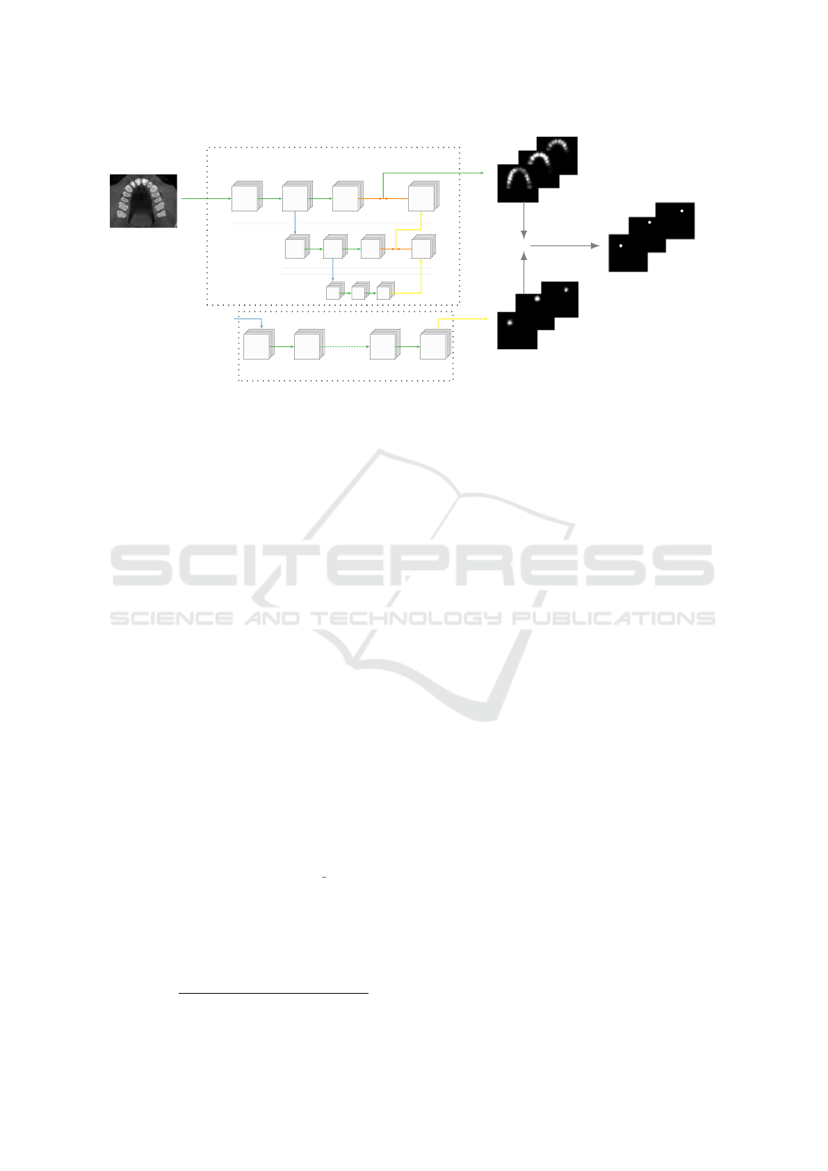
Figure 1: Teeth localization using SpatialConﬁguration-Net. The local appearance component generates a set of local appear-

ance heatmaps denoted as H

, while the spatial conﬁguration component produces a set of spatial conﬁguration heatmaps

. The ﬁnal heatmap images H for teeth landmarks are obtained by performing voxel-wise multiplication of H

and H

The arrows represent different operations: green arrow – convolution, blue arrow – downsampling, yellow arrow – upsam-

pling, and orange arrow – voxel-wise addition.

operations. After each convolutional layer we apply a

dropout of 0.3, and use ’same’ padding to maintain the

same input and output size. All layers have a ReLU

activation function except the last one, where no acti-

vation function is used in order to obtain logits instead

of probabilities as the network’s output. Same as for

the SCN, the weights in the last layer are initialized

with the He initializer. In all other layers, the initial

weights are sampled from a truncated normal distri-

bution with a standard deviation of 0.001. The last

layer consists of a single output, generating an image

with predicted intensity values. The network’s output

is an image of size [64, 64,64], with voxel intensities

in the range (−∞,+∞). Finally, a threshold of 0 was

applied to the output in order to produce the predicted

binary segmentation map, where all voxel values be-

low the threshold are considered background, while

non-negative values represent a detected lesion.

To address the class imbalance problem, we com-

pare three objective functions, Focal Loss FL (Lin

et al., 2017), Focal Tversky Loss FTL (Abraham and

Khan, 2019), and Combo Loss CL (Taghanaki et al.,

2019) based on Dice Similarity Coefﬁcient (DSC):

FL(p

) = −α

(1 − p

)

log(p

), (4)

FTL(P,G) = (1 − TI(P, G))

, (5)

and

CL(y, p) = δ · L

BBCE

(y, p) − (1 − δ) · DSC(y, p). (6)

In the above equations, Tversky Index (TI) and Bal-

anced Binary Cross-Entropy (BBCE) are deﬁned by

TI(P,G) =

|PG| + ε

|PG| + β|P\G| + (1 − β)|G\P| + ε

(7)

and

BBCE

(y, p) = −α· y log(p) − (1 − α) · (1 − y)log(1 − p).

(8)

The parameters α and β in the above equations are

used to weight positive and negative examples. α can

be set as the inverse class frequency or considered as a

hyperparameter, while values of β larger than 0.5 give

more signiﬁcance to false negative examples. To en-

hance the focus on misclassiﬁed predictions, γ should

be larger than 0 in the FL function and larger than 1

in the FTL function. The parameter δ regulates the

contribution of the BBCE to the CL function.

2.3 Data Augmentation

To prepare images for training the SCN for local-

ization, we resize all images from the original size

of [501, 501, 501] to a new size of [64,64,32], while

maintaining a ﬁxed aspect ratio. As we do not need

highly precise locations of teeth for the lesion seg-

mentation task, the SCN can be trained on downsam-

pled images. Image intensities are then scaled to the

range [−1,1]. Additionally, images undergo transla-

tion, rotation, and scaling using random factors sam-

pled from uniform distributions ([−10, 10] for trans-

lation, [−0.1,0.1] for rotation, [0.9,1.1] for scaling).

Before training our modiﬁed U-Net for the lesion

segmentation task, original high-resolution images

are cropped along with their corresponding ground

truth segmentation maps for each tooth. This process

generates 32 cropped images from a single original

image, where the center of each cropped image corre-

sponds to the center coordinate of a particular tooth.

Teeth Localization and Lesion Segmentation in CBCT Images Using SpatialConﬁguration-Net and U-Net

293

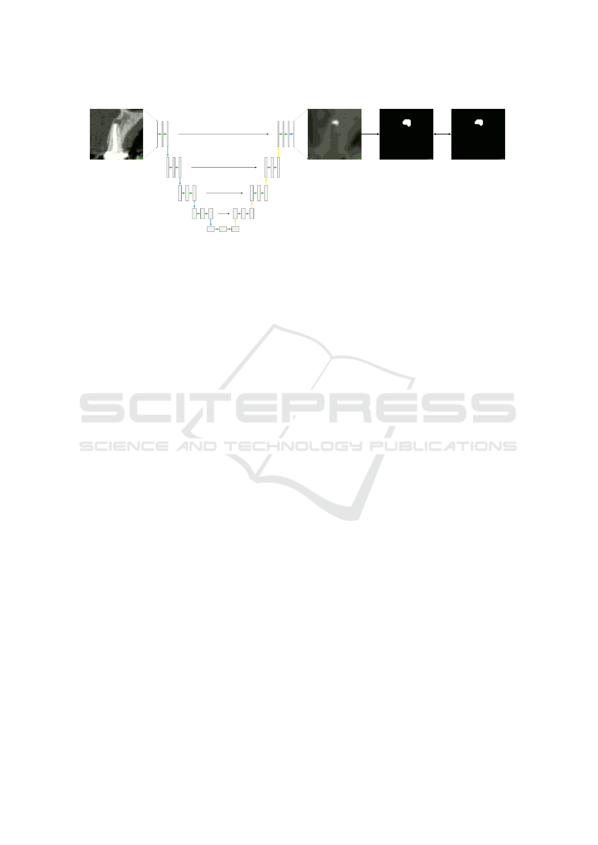
Input image

Output image

Predicted seg. map

Ground truth map

t = 0

U-Net

Figure 2: Periapical lesion segmentation using a modiﬁed U-Net architecture. A cropped image of a tooth along with its

corresponding ground truth map is used as input to the U-Net. The network is trained to output an image of intensity values,

where each value lies in the range (−∞, +∞). A threshold t is applied to the predicted intensity image in order to generate a

ﬁnal binary segmentation map.

Each cropped image has dimensions of [64,64,64]

and a spacing of [0.4,0.4,0.4]. Since periapical os-

teolytic lesions are always located in the area of the

root tips, we translate cropped images by ﬁxed fac-

tors to ensure visibility of the entire tooth root within

a cropped image. The translation factors of [0, 1, −9]

are applied to the cropped images with a tooth in

the upper jaw. The cropped images with a tooth in

the lower jaw are translated by factors [0,3,−9] and

rotated by 180 degrees. Moreover, all cropped im-

ages undergo random translation within the range of

[−1,−1], random rotation, and random scaling with-

ing the range of [−0.2, 0.2]. As a post-processing

step, we normalize cropped images to the range [0, 1]

and perform shift scale intensity transformation using

a random factor of 0.6. We perform label smoothing

by applying a Gaussian kernel with a standard devia-

tion of 0.1 to the ground truth segmentation maps.

2.4 Implementation Details

An Intel(R) CPU 920 with an NVIDIA GeForce GTX

TITAN X was used for the training and testing of the

model. The CNNs were running on Ubuntu 20.04

operating system with Python 3.7 and TensorFlow

1.15.0. To evaluate the performance of our model,

we used 4-fold cross validation (cv). Total training

time of the SCN for one cv fold took about 20 hours,

while one fold for training the U-Net took about 17

hours. The teeth localization network took around 15

seconds for inference on a CBCT volume, while the

segmentation network, including cropping, took ap-

proximately 2 to 3 minutes.

To minimize the loss function during training of

SCN, we use the Nesterov Accelerated Gradient with

a learning rate of 10e − 7 and momentum value of

0.99. We set the number of iterations to 15,000 as

we did not observe any substantial improvement after

that. Remaining hyper-parameters batch size, weight

decay, and sigma regularization term are determined

empirically and set to 1, 5e−5, and 100, respectively.

The U-Net is trained for 113,000 iterations using a

batch size of 8. As mentioned earlier, we address the

class imbalance issue by utilizing Focal Loss, Focal

Tversky Loss, and Combo Loss. We set the param-

eters of these loss functions as follows: Within our

dataset, positive voxels in each cropped image occupy

less than 10% of the volume. Therefore, we set the

weighting factors α and β to 0.9 in the corresponding

loss functions. The parameter γ controls the down-

weighting of easy examples. We set γ to 2 in the Focal

Loss and the Focal Tversky Loss function. In the case

of the Combo Loss function, we set the parameter δ

to 0.5, which determines the contribution of the Bal-

anced Binary Cross-Entropy. Furthermore, in order

to minimize the loss functions, we employ the Adam

optimizer with a learning rate of 1e − 4.

Both networks are trained and tested using the 4-

fold cross validation technique. For teeth localization,

our dataset of 144 3D CBCT images is divided into

four cv folds, each containing 36 images. For lesion

segmentation, we split a total of 2128 cropped images

into four cv folds. Since only 206 teeth in our dataset

are affected by a lesion, we distribute them uniformly

over all cv folds, resulting in 10% of teeth with lesions

and 90% teeth without lesions per fold.

2.5 Metrics

To evaluate the teeth localization performance, we

use the point-to-point error (PE) and accuracy met-

rics. For a landmark i, the point-to-point error PE

represents the Euclidean distance between the ground

truth landmark ˜x

and the predicted landmark x

′

. Ac-

VISAPP 2024 - 19th International Conference on Computer Vision Theory and Applications

294

curacy is deﬁned as the percentage of correctly identi-

ﬁed landmarks over all predicted landmarks (i.e., av-

erage precision). A predicted landmark x

′

is identiﬁed

correctly if the closest ground truth landmark is the

correct one and the Euclidean distance to the ground

truth landmark is less than a speciﬁed radius r.

To evaluate the lesion detection performance, we

use the metrics sensitivity (TP/(TP+FN)) and speci-

ﬁcity (TN/(TN + FP)). Each predicted segmentation

is evaluated based on the Dice score, an overlap mea-

sure between the ground truth segmentation map X

and the predicted segmentation map Y , deﬁned by

DSC = 2 ·

|X ∩Y |

|X| + |Y |

. (9)

Sensitivity represents the network’s ability to cor-

rectly detect teeth with lesions, whereas speciﬁcity

represents its ability to correctly detect teeth without

lesions. A predicted segmentation map for a tooth

with a lesion is classiﬁed as a True Positive (TP) if

the Dice score between the ground truth and predicted

segmentation map is larger than 0. Otherwise, the pre-

dicted segmentation map is classiﬁed as a False Neg-

ative (FN). A predicted segmentation map for a tooth

without a lesion is classiﬁed as a True Negative (TN)

if all voxels in the predicted segmentation map are 0.

Otherwise, the predicted segmentation map is classi-

ﬁed as a False Positive (FP) prediction.

2.6 Delaunay Triangulation

For the training of the U-Net, each original image

is cropped to the size of [64,64,64] for each tooth,

where the center coordinate of a cropped image corre-

sponds to the center coordinate of the particular tooth

in the original image. Since teeth can have different

shapes, sizes, and orientations, the resulting cropped

images may contain multiple teeth, which compli-

cates automated tooth-based evaluation. To address

this issue, we use the deﬁnitions of the convex hull

and the Delaunay triangulation.

First, we annotate a cuboid around each tooth in

the original image using Planmeca Romexis

soft-

ware. This annotation ensures that each cuboid en-

closes only the area of a single tooth. The software

then automatically generates a set of 3D coordinates

representing the cuboid. We use these coordinates as

input for the ’Convex-Hull’ and ’Delaunay’ functions

from the SciPy 1.6.2 library. By using the ’Delau-

nay.ﬁnd simplex’ function, we obtain the indices of

all the simplices that contain all cuboid voxels. Using

these indices, we are able to generate a segmentation

map for an annotated cuboid. Finally, during the eval-

uation of a speciﬁc tooth, we only consider the voxels

that belong to its corresponding annotated cuboid.

3 RESULTS AND DISCUSSION

The results of the teeth localization and lesion seg-

mentation tasks are shown in Table 1 and Table 2, re-

spectively. Moreover, we provide a comparison of the

results with SOTA methods for periapical lesion de-

tection in Table 3.

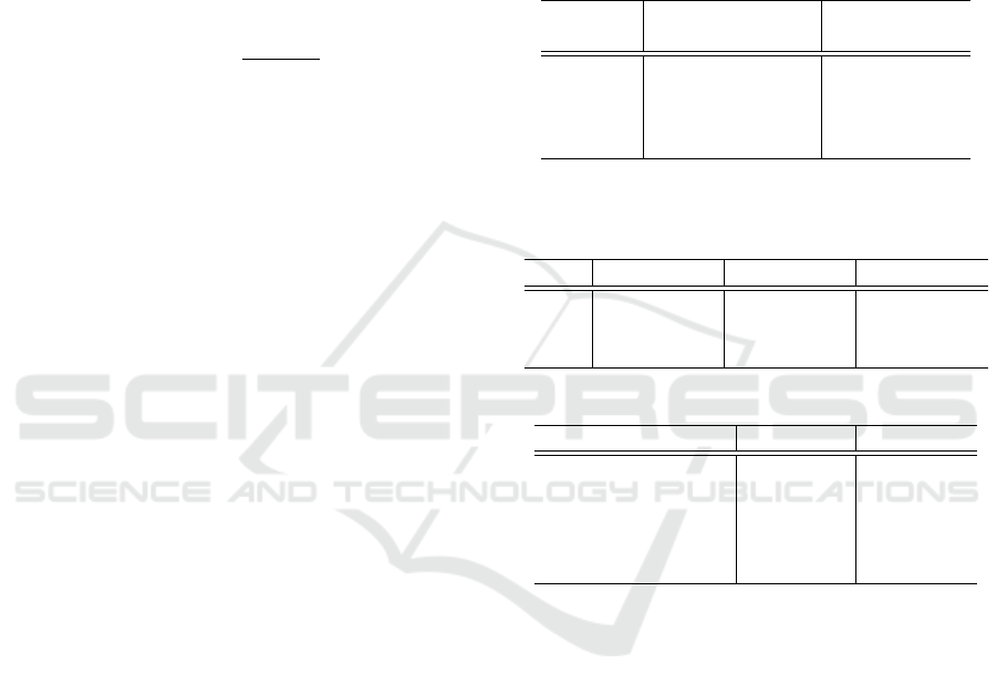
Table 1: Teeth localization results for 4-fold cross valida-

tion, showing point-to-point error with standard deviation,

as well as accuracy of the model for different radii r.

Radius r

PE in mm

Accuracy (%)

Mean ± SD

2 mm











72.6

3 mm 1.74 ± 1.44 89.1

4 mm 94.7

6 mm 97.3

Table 2: Lesion detection and segmentation results for 4-

fold cross validation, shown as sensitivity, speciﬁcity, and

Dice score obtained using different loss functions.

Loss Sensitivity Speciﬁcity DICE

FL 0.97 ± 0.03 0.88 ± 0.04 0.67 ± 0.03

FTL 0.92 ± 0.05 0.89 ± 0.08 0.70 ± 0.04

CL 0.85 ± 0.04 0.94 ± 0.02 0.70 ± 0.04

Table 3: Comparison with SOTA methods.

Method Sensitivity Speciﬁcity

(Lee et al., 2020) 0.94 -

(Setzer et al., 2020) 0.93 0.88

(Zheng et al., 2020) 0.84 -

(Orhan et al., 2020) 0.93 -

Ours 0.97 0.88

We evaluated the performance of the SCN on 4

folds and achieved an average accuracy of 97.3% in

teeth detection, with a mean point-to-point error of

1.74 ± 1.44 mm. In other words, for 97.3% of the

predicted teeth, the closest ground truth landmark was

the correct one and the distance between the predicted

and ground truth landmarks was less than 6 mm. De-

creasing the radius to 4, 3, and 2 mm resulted in av-

erage accuracy values of 94.7%, 89.1%, and 72.6%,

respectively. By observing individual predictions, we

could notice that the most incorrect predictions oc-

curred in images affected by artifacts or images with

misaligned teeth. This can be attributed to these cases

being rare in our dataset and thus deviating from the

learned data distribution. In future work, this could

be addressed by combining generative models with

CNNs to incorporate global shape/landmark conﬁgu-

rations into the training process. This way, the detec-

tion of out-of-distribution data could be improved.

Teeth Localization and Lesion Segmentation in CBCT Images Using SpatialConﬁguration-Net and U-Net

295

The U-Net was trained using the Focal Loss (FL),

Focal Tversky Loss (FTL), and Combo Loss (CL)

functions. By adjusting the parameters of these loss

functions, we were able to reweight the hard and easy

class examples. Each setup was evaluated on 4 folds,

with uniformly distributed teeth with lesions. The

highest lesion detection rate of 0.97 was achieved

using FL, whereas FTL and CL achieved the detec-

tion rates of 0.92 and 0.88, respectively. The high-

est speciﬁcity value of 0.94 was achieved using CL,

while the values of 0.88 and 0.89 were achieved us-

ing FL and FTL, respectively. The highest Dice score

of 0.70 was achieved using the FTL and CL func-

tions. The setup trained with FL achieved a slightly

smaller value of 0.66 for the Dice score. By observ-

ing the predictions for individual lesions, we noticed

a larger number of false negative predicted voxels and

consequently lower Dice scores in images with very

small or very large lesions. Small differences between

predicted and ground truth segmentation maps have a

signiﬁcant impact on the Dice score for images with

very small lesions, while a signiﬁcant predicted por-

tion of a lesion can result in a low Dice score for

images with very large lesions. Since false negative

predictions are less tolerable than false positive pre-

dictions in the lesion detection task, we conclude that

the best performance of our method was achieved us-

ing the FL function with a sensitivity value of 0.97

and a speciﬁcity value of 0.88. In future work, we

plan to explore the use of stronger anatomical con-

straints via generative models to improve the crucial

teeth localization step.

When comparing our method with other SOTA

methods, our approach achieved the highest sensitiv-

ity value and the same speciﬁcity value as (Setzer

et al., 2020). However, it is important to note that

a direct comparison is not feasible due to the use of

different datasets in the evaluation of these methods.

Furthermore, all SOTA methods, except (Orhan et al.,

2020), utilized 2D slices rather than 3D volumes dur-

ing the training and testing procedures. Addition-

ally, the studies conducted in (Setzer et al., 2020) and

(Zheng et al., 2020) were limited to small respective

datasets. When considering the negative class, which

refers to teeth without periapical lesions, only (Setzer

et al., 2020) reported a speciﬁcity value. However,

their dataset is highly selective as it consists of only

20 CBCT volumes with limited ﬁeld-of-view. More-

over, among these volumes, there are 29 roots with le-

sions and 32 roots without lesions, thus creating a bal-

anced distribution of roots with and without lesions,

which does not reﬂect clinical practice.

4 CONCLUSION

In this paper, we have presented a fully automated

two-step method for detecting periapical lesions in

CBCT images. In the ﬁrst step, we utilize the 3D

SpatialConﬁguration-Net (SCN) for teeth localiza-

tion. By using the teeth coordinates generated by the

SCN, we extract relevant subregions from the original

images, and use them to train the 3D U-Net for lesion

segmentation in the second step. In contrast to other

SOTA methods, our method incorporates 3D volumes

throughout all stages, ensuring no loss of valuable in-

formation. Additionally, to the best of our knowledge,

we are the ﬁrst to address the class imbalance issue

associated with automatic periapical lesion detection,

which is commonly observed in clinical data. De-

spite the challenges posed by dental CBCT images,

our method achieved promising results in localizing

teeth and detecting periapical lesions in CBCT data.

REFERENCES

Abraham, N. and Khan, N. M. (2019). A novel focal

Tversky loss function with improved Attention U-

Net for lesion segmentation. In 2019 IEEE 16th In-

ternational Symposium on Biomedical Imaging (ISBI

2019), pages 683–687. IEEE.

Antony, D. P., Thomas, T., and Nivedhitha, M. (2020). Two-

dimensional periapical, panoramic radiography versus

three-dimensional cone-beam computed tomography

in the detection of periapical lesion after endodontic

treatment: A systematic review. Cureus, 12(4).

Chung, M., Lee, M., Hong, J., Park, S., Lee, J., Lee, J.,

Yang, I.-H., Lee, J., and Shin, Y.-G. (2020). Pose-

aware instance segmentation framework from cone

beam ct images for tooth segmentation. Computers

in Biology and Medicine, 120:103720.

Cootes, T. F., Hill, A., Taylor, C. J., and Haslam, J. (1994).

Use of active shape models for locating structures

in medical images. Image and Vision Computing,

12(6):355–365.

Donner, R., Menze, B. H., Bischof, H., and Langs, G.

(2013). Global localization of 3d anatomical struc-

tures by pre-ﬁltered hough forests and discrete opti-

mization. Medical Image Analysis, 17(8):1304–1314.

Du, M., Wu, X., Ye, Y., Fang, S., Zhang, H., and Chen,

M. (2022). A combined approach for accurate and

accelerated teeth detection on cone beam ct images.

Diagnostics, 12(7):1679.

Ekert, T., Krois, J., Meinhold, L., Elhennawy, K., Emara,

R., Golla, T., and Schwendicke, F. (2019). Deep learn-

ing for the radiographic detection of apical lesions.

Journal of Endodontics, 45(7):917–922.

Endres, M. G., Hillen, F., Salloumis, M., Sedaghat, A. R.,

Niehues, S. M., Quatela, O., Hanken, H., Smeets, R.,

Beck-Broichsitter, B., Rendenbach, C., et al. (2020).

VISAPP 2024 - 19th International Conference on Computer Vision Theory and Applications

296

Development of a deep learning algorithm for peri-

apical disease detection in dental radiographs. Diag-

nostics, 10(6):430.

Gan, Y., Xia, Z., Xiong, J., Li, G., and Zhao, Q. (2017).

Tooth and Alveolar Bone Segmentation From Den-

tal Computed Tomography Images. IEEE Journal of

Biomedical and Health Informatics, 22(1):196–204.

He, K., Zhang, X., Ren, S., and Sun, J. (2015). Delving

deep into rectiﬁers: Surpassing human-level perfor-

mance on ImageNet classiﬁcation. In Proceedings of

the IEEE International Conference on Computer Vi-

sion, pages 1026–1034.

Heimann, T. and Meinzer, H.-P. (2009). Statistical shape

models for 3D medical image segmentation: A review.

Medical Image Analysis, 13(4):543–563.

Jain, A., Tompson, J., Andriluka, M., Taylor, G. W., and

Bregler, C. (2014). Learning human pose estima-

tion features with convolutional networks. In 2nd In-

ternational Conference on Learning Representations

(ICLR), pages 1–11.

Khanagar, S. B., Al-Ehaideb, A., Vishwanathaiah, S., Ma-

ganur, P. C., Patil, S., Naik, S., Baeshen, H. A., and

Sarode, S. S. (2021). Scope and performance of ar-

tiﬁcial intelligence technology in orthodontic diagno-

sis, treatment planning, and clinical decision-making-

a systematic review. Journal of Dental Sciences,

16(1):482–492.

Kirnbauer, B., Hadzic, A., Jakse, N., Bischof, H., and Stern,

D. (2022). Automatic detection of periapical oste-

olytic lesions on cone-beam computed tomography

using deep convolutional neuronal networks. Journal

of Endodontics, 48(11):1434–1440.

Krois, J., Garcia Cantu, A., Chaurasia, A., Patil, R., Chaud-

hari, P. K., Gaudin, R., Gehrung, S., and Schwen-

dicke, F. (2021). Generalizability of deep learning

models for dental image analysis. Scientiﬁc Reports,

11(1):6102.

Lee, J.-H., Kim, D.-H., and Jeong, S.-N. (2020). Diagno-

sis of cystic lesions using panoramic and cone beam

computed tomographic images based on deep learn-

ing neural network. Oral Diseases, 26(1):152–158.

Lin, T., Goyal, P., Girshick, R. B., He, K., and Doll

ar, P.

(2017). Focal loss for dense object detection. In IEEE

International Conference on Computer Vision, pages

2999–3007. IEEE.

Orhan, K., Bayrakdar, I., Ezhov, M., Kravtsov, A., and

Ozy

urek, T. (2020). Evaluation of artiﬁcial intelli-

gence for detecting periapical pathosis on cone-beam

computed tomography scans. International Endodon-

tic Journal, 53(5):680–689.

Pauwels, R., Brasil, D. M., Yamasaki, M. C., Jacobs, R.,

Bosmans, H., Freitas, D. Q., and Haiter-Neto, F.

(2021). Artiﬁcial intelligence for detection of periapi-

cal lesions on intraoral radiographs: Comparison be-

tween convolutional neural networks and human ob-

servers. Oral Surgery, Oral Medicine, Oral Pathology

and Oral Radiology, 131(5):610–616.

Payer, C., Stern, D., Bischof, H., and Urschler, M. (2019).

Integrating spatial conﬁguration into heatmap regres-

sion based CNNs for landmark localization. Medical

Image Analysis, 54:207–219.

Payer, C., Stern, D., Bischof, H., and Urschler, M. (2020).

Coarse to ﬁne vertebrae localization and segmentation

with SpatialConﬁguration-Net and U-Net. In VISI-

GRAPP (5: VISAPP), pages 124–133.

Ronneberger, O., Fischer, P., and Brox, T. (2015). U-

net: Convolutional networks for biomedical im-

age segmentation. In Medical Image Computing

and Computer-Assisted Intervention – MICCAI 2015,

pages 234–241. Springer International Publishing.

Setzer, F. C., Shi, K. J., Zhang, Z., Yan, H., Yoon, H., Mup-

parapu, M., and Li, J. (2020). Artiﬁcial intelligence

for the computer-aided detection of periapical lesions

in cone-beam computed tomographic images. Journal

of Endodontics, 46(7):987–993.

Taghanaki, S. A., Zheng, Y., Zhou, S. K., Georgescu, B.,

Sharma, P., Xu, D., Comaniciu, D., and Hamarneh, G.

(2019). Combo loss: Handling input and output im-

balance in multi-organ segmentation. Computerized

Medical Imaging and Graphics, 75:24–33.

Umer, F. and Habib, S. (2022). Critical analysis of artiﬁcial

intelligence in endodontics: a scoping review. Journal

of Endodontics, 48(2):152–160.

Unterpirker, W., Ebner, T.,

Stern, D., and Urschler, M.

(2015). Automatic third molar localization from 3D

MRI using random regression forests. In 19th Interna-

tional Conference on Medical Image Understanding

and Analysis (MIUA), pages 195–200, Lincoln, UK.

Urschler, M., Ebner, T., and

Stern, D. (2018). Integrating

geometric conﬁguration and appearance information

into a uniﬁed framework for anatomical landmark lo-

calization. Medical Image Analysis, 43:23–36.

Urschler, M., Leitinger, G., and Pock, T. (2014). Interac-

tive 2D/3D image denoising and segmentation tool for

medical applications. In Proceedings MICCAI Work-

shop Interactive Medical Image Computation (IMIC).

Yushkevich, P. A., Piven, J., Cody Hazlett, H., Gim-

pel Smith, R., Ho, S., Gee, J. C., and Gerig, G.

(2006). User-guided 3D active contour segmentation

of anatomical structures: Signiﬁcantly improved efﬁ-

ciency and reliability. Neuroimage, 31(3):1116–1128.

Zhang, J., Liu, M., and Shen, D. (2017). Detecting

anatomical landmarks from limited medical imaging

data using two-stage task-oriented deep neural net-

works. IEEE Transactions on Image Processing,

26(10):4753–4764.

Zheng, Z., Yan, H., Setzer, F. C., Shi, K. J., Mupparapu,

M., and Li, J. (2020). Anatomically constrained deep

learning for automating dental cbct segmentation and

lesion detection. IEEE Transactions on Automation

Science and Engineering, 18(2):603–614.

Teeth Localization and Lesion Segmentation in CBCT Images Using SpatialConﬁguration-Net and U-Net

297