Group Importance Estimation Method

Based on Group LASSO Regression

Yuki Mori

1 a

, Seiji Yamada

2 b

and Takashi Onoda

1 c

Aoyama Gakuin University School of Science and Engineering, 5-10-1 Huchinobe, Chuo, Sagamihara, Kanagawa, Japan

National Institute of Informatics 2-1-2 Hitotsubashi, Chiyoda, Tokyo, Japan

Keywords:

Group LASSO Regression, Machine Learning, LASSO Regression, Group Variable Selection, Estimate

Group Importance, Linear Regression Problem, Penalized Least Squares Problem.

Abstract:

There has been a rapidly growing interest in penalized least squares problems via l

regularization. The

LASSO (Least Absolute Shrinkage and Selection Operator) regression, which utilizes l

regularization, has

gained popularity as a method for model selection and shrinkage estimation. An important extension of

LASSO regression is Group LASSO regression, which generates sparse models at the group level. However,

Group LASSO regression does not directly evaluate group importance. In this study, we propose a method

to assess group importance based on Group LASSO regression. This method leverages regularization param-

eters to estimate the importance of each group. We applied this method to both synthetically generated data

and real-world data, conducting experiments to evaluate its performance. As a result, the method accurately

approximated the importance of groups, enhancing the interpretability of models at the group level.

1 INTRODUCTION

Recently, there has been a rapidly growing interest

in penalized least squares problems via l

regulariza-

tion(Nardi and Rinaldo, 2008). The LASSO (Least

Absolute Shrinkage and Selection Operator) regres-

sion(Tibshirani, 1996) is a regularization technique

where the penalty for model complexity is the l

norm of the estimated coefﬁcients. Originally devel-

oped for linear regression models, LASSO regression

has gained popularity as a method for model selec-

tion and shrinkage estimation. Group LASSO regres-

sion(Yuan and Lin, 2006), which selects key explana-

tory factors in a grouped manner, is an important ex-

tension of LASSO regression(Yang et al., 2010).This

method has found successful applications in various

ﬁelds, including birthweight prediction and gene ﬁnd-

ing(Yuan and Lin, 2006)(Meier et al., 2008). How-

ever, while it can yield solutions with sparsity at the

group level, it doesn’t inherently assess the individual

group importance. In this study, we propose to assess

group importance based on Group LASSO regression,

thereby enhancing interpretability and addressing the

https://orcid.org/0009-0007-9122-629X

https://orcid.org/0000-0002-5907-7382

https://orcid.org/0000-0002-5432-0646

limitations of the existing approach.

In the subsequent section of this paper, we delve

into Group LASSO regression. In section 3, we detail

the proposed method for estimating group importance

based on Group LASSO regression. Moving to sec-

tion 4, we engage in experimental validations, testing

the efﬁcacy of our approach using both synthetically

generated data and real data. Finally, we conclude by

summarizing the key ﬁndings of our study and dis-

cussing the adaptability of our proposed approach in

real-world scenarios.

2 GROUP LASSO REGRESSION

In this section, we present Group LASSO regres-

sion(Yuan and Lin, 2006) and proximal gradient al-

gorithms for Group LASSO regression(Tomioka and

Scientiﬁc, 2015).

Consider a linear model where we have in-

dependent and identically distributed observations

(1)i

,··· ,x

(M)i

),i = 1,··· ,N, of a N-dimensional

vector⃗x

= (x

(k)1

,··· ,x

(k)N

)

⊤

,⃗y = (y

,··· ,y

)

⊤

, ma-

trix X = (⃗x

,··· ,⃗x

) and the parameter vector

⃗

β ∈

, which holds the coefﬁcients for each feature. The

relationship between the features and the response in

Mori, Y., Yamada, S. and Onoda, T.

Group Importance Estimation Method Based on Group LASSO Regression.

DOI: 10.5220/0012304800003654

Paper published under CC license (CC BY-NC-ND 4.0)

In Proceedings of the 13th International Conference on Pattern Recognition Applications and Methods (ICPRAM 2024), pages 197-204

ISBN: 978-989-758-684-2; ISSN: 2184-4313

197

this model is given by:

⃗y = X

⃗

β +

⃗

ε (1)

Here,

⃗

ε ∈ R

is the error vector capturing the devia-

tion from the linear model, assumed to be independent

and identically distributed, following a normal distri-

bution with mean 0.

In the context of Group LASSO Regression, we

extend this basic linear model to accommodate a

structure where the M features are partitioned into

J distinct groups. Let m

denote the number of fea-

tures in the j-th group. Consequently, matrix X can

be expressed as X = (X

,··· ,X

) where X

∈ R

N×m

The coefﬁcient vector

⃗

β is similarly decomposed into

⃗

β = (

⃗

,··· ,

⃗

)

⊤

, where

⃗

= (β

{ j}1

,··· ,β

{ j}m

) for

j = 1,··· ,J.

The optimization problem for Group LASSO,

considering the above model, is deﬁned as:

min

⃗

∥⃗y − X

⃗

β∥

+ λ

∑

j=1

∥

⃗

∥

(2)

In this formulation, ∥

⃗

∥

represents the l

norm

of the coefﬁcients of the j-th group, calculated as

∥

⃗

∥

∑

p=1

{ j}p

. The parameter λ is a non-

negative regularization term that introduces group-

wise sparsity into the model, effectively encouraging

the model to reduce the coefﬁcients of less relevant

groups to zero. This results in a more parsimonious

and interpretable model that highlights the most sig-

niﬁcant group-based features for predicting the target

variable.

We also introduce the proximal gradient algo-

rithm, an iterative optimization technique used for

addressing both convex and non-convex optimization

problems, including LASSO regression and Group

LASSO regression. It updates the differentiable com-

ponents similarly to gradient descent and handles the

non-differentiable components using the proximal op-

erator. The update formula for the proximal gradient

algorithm is given by the following expression, which

incorporates the proximal operator:

⃗

(t+1)

= prox(

⃗

(t)

− γ∇ f (

⃗

(t)

)) (3)

where,

⃗

(t)

represents the regression coefﬁcients

⃗

β up-

dated at the t-th iteration, γ is the step size and ∇ f (

⃗

β)

denotes the gradient of the function f (

⃗

β), which is a

differentiable convex function. The convergence cri-

teria used in the proximal gradient algorithm are as

follows:

||F(

⃗

(t+1)

) −F(

⃗

(t)

)||

||F(

⃗

(t+1)

)||

< e ≈ 0 (4)

Input: X , ⃗y, λ, γ

Initialization: t = 0 and

⃗

(t)

⃗

(0)

while not satisﬁed with Equation (4) do

Calculate the gradient: ∇ f (

⃗

(t)

)

Update the

⃗

β based on Equation (3) and

Equation (7)

Update t = t + 1

end

Output:

⃗

(t)

Algorithm 1: Proximal Gradient Algorithm for

Group LASSO Regression.

where, F(

⃗

β) represents the objedtive function, which

is a convex function and e denotes a small constant

close to zero. In Group LASSO regression, F(

⃗

β) and

f (

⃗

β) are deﬁned as:

⃗

β) =

||⃗y − X

⃗

β||

+ λ

∑

j=1

⃗

(5)

f (

⃗

β) =

||⃗y − X

⃗

β||

(6)

Furthermore, in Group LASSO regression, the prox-

imal operator is deﬁned using the proximity point

⃗

′

∈ R

as follows:

prox(

⃗

′

) =







⃗

′

−

γλ

⃗

′

⃗

′

⃗

′

≥ γλ

0 ||

⃗

′

< γλ

(7)

Based on the equations presented in section 2, Algo-

rithm 1 shows the ﬂow of the proximal gradient algo-

rithm for Group LASSO regression.

3 GROUP IMPORTANCE

ESTIMATION METHOD

In this section, we propose the group importance es-

timation method based on Group LASSO regression.

Section 3.1 lays the foundation by explaining the core

concepts of our method. Following that, section 3.2

sheds light on the importance of the threshold in our

approach. Finally, section 3.3 provides a comprehen-

sive formulation of the proposed method.

3.1 Concept of the Group Importance

Estimation

While Group LASSO regression is powerful in

achieving sparsity at the group level, it often side-

lines the assessment of individual group importance.

ICPRAM 2024 - 13th International Conference on Pattern Recognition Applications and Methods

198

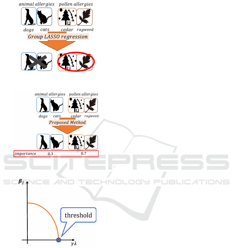
Figure 1: Example of allergy diagnosis for Group LASSO

regression.

Figure 2: Example of allergy diagnosis for proposed

method.

Figure 3: Illustrative representation of the relationship be-

tween

⃗

and λ.

For illustration, consider an allergy diagnosis sce-

nario where the goal is to predict reactions to speciﬁc

allergens. The predictions hinge on various symp-

toms, ranging from allergies to dogs and cats (cate-

gorized as animal allergies) to cedar pollen and rag-

weed (grouped under pollen allergies). When em-

ploying Group LASSO regression in such a context,

the group variable selection might look like what’s

shown in Fig. 1. In this ﬁgure, ”×” indicates that the

regression coefﬁcients for animal allergies are zero,

suggesting that this group’s variables have been ex-

cluded. In contrast, ”⃝” signals the presence of non-

zero coefﬁcients for pollen allergies, indicating their

incorporation in the regression model. A quick look

at Fig. 1 might suggest that pollen allergies play a piv-

otal role in the regression model. However, the cur-

rent approach falls short in offering a nuanced com-

parison between the importance of animal and pollen

allergies. Addressing this gap, our study proposes a

method to assess the importance of such groups, as

shown in Fig. 2.

Central to our method is the establishment of

a common criterion to assess the relative impor-

tance of each group. To achieve this, we explore a

methodology that utilizes the threshold for determin-

ing whether a group is important or not in predicting

the target variable. This threshold serves as a com-

mon criterion derived from the feature selection pro-

cess conducted at the group level in Group LASSO

regression. With the general concept of our method

outlined, we’ll now delve deeper into the pivotal role

the threshold plays in our approach.

3.2 Threshold for the Group

Importance Estimation

A group j is considered important in predicting the

target variable if

⃗

̸=

⃗

0, and unimportant if

⃗

As brieﬂy described in Algorithm 1 in Section 2, if

the condition ||

⃗

′

< γλ holds according to Equa-

tion (7), then

⃗

0, leading to the elimination of

variables within group j. Conversely, if the condition

⃗

′

> γλ holds, then

⃗

̸=

⃗

0, and as a result,

variables within group j are not reduced. Essentially,

the value of γλ has an impact on variable selection

at the group level. In this study, Fig. 3 shows

the relationship between

⃗

and λ. Based on this

depiction, we consider the point where

⃗

0 is ﬁrst

achieved as a threshold common to each group. For

this boundary to exist in all groups, the relationship

between

⃗

and γλ must be either monotonically

increasing or decreasing. To shed more light on this,

we experimentally verify the relationship between

⃗

and γλ. Since γ is provided as a constant,

we use a path diagram to clarify this relationship

between ||

⃗

and λ.

Experimental Conditions.

For the vector ⃗v[θ, η], we deﬁne:

1000

∑

n=1

⃗v[θ, η]

= θ,

1000

∑

n=1

⃗v[θ, η]

= η

Group Importance Estimation Method Based on Group LASSO Regression

199

From this, we derive the vector ⃗x

as:

⃗x

=⃗v[0,1] (m = 1,··· ,9)

The target variable, ⃗y, is then generated as:

⃗y = X

⃗

β +⃗v[0, 2]

The regression coefﬁcient vectors

⃗

, and

⃗

are

deﬁned as:

⃗

= (1.0,1.0,1.0)

⃗

= (2.0,2.0,2.0)

⃗

= (3.0,3.0,3.0)

Combining these, the regression coefﬁcient vector

⃗

is:

⃗

β = (

⃗

)

⊤

Furthermore, standardization is applied to X, and ⃗x

is centered (mean 0). By varying the value of the reg-

ularization parameter λ in the range [10

−1

,10

], we

aim to show the relationship between ||

⃗

and λ.

Fig. 4 shows a path diagram that captures this re-

lationship. Fig. 4 shows that ”Overall” represents

⃗

β||

, ”Group1” is ||

⃗

, ”Group2” is ||

⃗

, and

”Group3” is ||

⃗

. It’s evident from the ﬁgure that

⃗

decreases monotonically as λ grows. Next,

based on Algorithm 1, we will explore the relation-

ship between ||

⃗

and λ. From Equation (3) and

Equation (7) in Algorithm 1, it becomes clear that

as λ increases, the value of ||

⃗

is updated to be-

come smaller. Therefore, we can infer that there is

a monotonically increasing or decreasing relationship

between ||

⃗

and λ. However, due to the conver-

gence conditions in Equation (4), there might be sce-

narios where this relationship doesn’t hold. Thus,

the relationship between ||

⃗

and λ is not strictly

monotonic. However, instances where this relation-

ship does not hold are rare. From the above discus-

sions, it’s clear that a general monotonic relationship,

either increasing or decreasing, exists between ||

⃗

and λ. Based on this understanding, in this study, we

assume that either a monotonic decreasing or increas-

ing relationship exists between λ and ||

⃗

. Fur-

thermore, based on the above analysis, we use the

threshold to estimate the importance of each group

in predicting the target variable as a criterion for es-

tablishing their relative importance in this study. No-

tably, the key factor that distinguishes among differ-

ent groups is the value of the regularization parame-

ter λ at this threshold. Therefore, by leveraging the

value of the regularization parameter λ at the thresh-

old for each group, we can estimate the importance of

each group, thereby improving the interpretability of

group-speciﬁc data.

Step 1: Prepare multiple values of the

regularization parameter λ to identify the

threshold in group j that determines whether

it is important or not for predicting the

target variable.

Step 2: Deﬁne the optimization problem as

outlined in Equation 2. Estimate the

regression coefﬁcient

⃗

β using the proximal

gradient algorithm for Group LASSO

Regression (Algorithm 1).

Step 3: If the regression coefﬁcient

⃗

estimated in Step 2 is not the zero vector,

calculate the value of ||

⃗

− γλ. The

regularization parameter λ that is closest to

calculating ||

⃗

− γλ ≈ 0 is deﬁned as λ

Step 4: Convert λ

into a ratio and estimate

group importance using the formula given in

Equation (8).

Algorithm 2: Group Importance Estimation based

on Group LASSO Regression.

Figure 4: Relationship between the regularization parame-

ter λ and group coefﬁcient ||

⃗

3.3 Formulation of the Group

Importance Estimation

In the proposed method, we utilize the optimization

problem of Group LASSO regression, represented by

Equation (2). We consider the point where the group

regression coefﬁcient

⃗

ﬁrst becomes zero as the

group’s threshold, as detailed in section 3.2.

To effectively implement our proposed method, it

is essential to identify the threshold for the group by

adjusting the value of the regularization parameter λ.

However, pinpointing this threshold accurately is a

complex task. Speciﬁcally, there’s a need to search

through the values of λ in ﬁne-grained steps to de-

termine the threshold for the group with precision.

Such an approach might substantially increase com-

putational time, potentially rendering it impractical

ICPRAM 2024 - 13th International Conference on Pattern Recognition Applications and Methods

200

for large datasets or real-time applications. Therefore,

to address this challenge, instead of using the point at

which the regression coefﬁcient for a group,

⃗

, ﬁrst

becomes zero as the threshold, we propose estimating

the threshold near the point where

⃗

ﬁrst becomes

zero. Building on this, the essence of our approach

can be captured from Equation (7). If γλ > ||

⃗

remains non-zero. Conversely, if γλ < ||

⃗

becomes zero. This implies that γλ = ||

⃗

serves

as a crucial threshold in our framework. For our

study, we adopt γλ ≈ ||

⃗

as the threshold for the

group. Further, to estimate this threshold, we compute

multiple regression coefﬁcients

⃗

β for varied λ values.

Our objective is to locate the threshold ||

⃗

≈ γλ

where

⃗

β remains non-zero. With γ being constant

at this threshold, λ provides a measure of group im-

portance. We deﬁne λ

for each group j such that

⃗

≈ γλ. This value, λ

, is indicative of the im-

portance of group j in our proposed method.

To facilitate a more comprehensive comparison

among groups, we introduce an importance measure

, which quantiﬁes the relative importance of group

j. Formally, it is deﬁned as:

∑

k=1

(8)

A thorough step-by-step explanation of this method is

provided in Algorithm 2.

4 EXPERIMENTS

In this section, we conduct experiments using both

generated data and real data to demonstrate the ef-

ﬁcacy of the estimated group importance using our

proposed method. Section 4.1 provides a detailed

description of the generated and real-world datasets.

Section 4.2 presents the common experimental con-

ditions for both sets of experiments. Finally, section

4.3 shows the results from both the generated and real

data experiments.

4.1 Experimental Data

4.1.1 Generated Data

We generated data using speciﬁc parameters. For the

vector⃗v[θ, η], we deﬁne:

400

∑

n=1

⃗v[θ, η]

= θ,

400

∑

n=1

⃗v[θ, η]

= η

From this, we derive the vector ⃗x

as:

⃗x

=⃗v[0,1] (m = 1,··· ,15)

The target variable, ⃗y, is then generated as:

⃗y = X

⃗

β +⃗v[0, 2]

The regression coefﬁcients

⃗

β are detailed in Table 1.

As indicated in Table 1, the coefﬁcients for group 1,

⃗

, are deﬁned as β

{1}m

= 0.4 for m

= 1, 2, 3. By

setting the elements of the regression coefﬁcients for

each group to the same value in this experiment, the

values presented in the third row of Table 1 represent

the importance of each group.

4.1.2 Real Data

The data utilized in this study is sourced from the

open datasets made publicly available by the Ministry

of Health, Labour and Welfare in Japan. Our experi-

ments span data points collected from May 10, 2020,

to May 8, 2023, totaling 1094 entries. The target vari-

able (or the dependent variable) is the number of daily

deaths in Japan due to the novel coronavirus (COVID-

19) infection. The independent variables (or explana-

tory variables) represent the number of daily infec-

tions with the COVID-19, broken down by prefecture

in Japan. Out of all the prefectures, 12 were selected

for this study based on the criterion that they ac-

counted for at least 2% of the total infections in Japan

as of May 8, 2023. These prefectures are Hokkaido,

Saitama, Chiba, Tokyo, Kanagawa, Shizuoka, Aichi,

Kyoto, Osaka, Hyogo, Hiroshima, and Fukuoka. The

rationale behind this selection is to ensure the model’s

appropriateness by avoiding prefectures with signif-

icantly low infection rates compared to the national

total as of May 8, 2023.

In Japan, prefectures are often categorized into

regions: Hokkaido, Tohoku, Kanto, Chubu, Kinki,

Chugoku, Shikoku, Kyushu, and Okinawa. To deﬁne

the group importance in our experiments, we used the

total number of deaths due to COVID-19 as of May 8,

2023, in the selected 12 prefectures. We then aggre-

gated these death counts according to the aforemen-

tioned regional groupings. The rationale behind using

the total number of deaths in each region is to provide

an estimate of the group’s importance in each area.

By utilizing the total death count, we can indicate the

severity and impact of the pandemic in each region,

which serves as an approximation of the group’s im-

portance. The deﬁned group importance is presented

in the fourth column of Table 2.

In this study, we conducted statistical tests us-

ing Ridge regression to assess whether the real data

is suitable for the regression model. Speciﬁcally,

we evaluated whether the model’s residuals were ho-

moscedastic by conducting the Breusch-Pagan test.

The results showed a p-value of 0.078, indicating

Group Importance Estimation Method Based on Group LASSO Regression

201

Table 1: Regression coefﬁcients and Group importance in generated data.

Coefﬁcient

⃗

{1}1

{1}2

{1}3

{2}1

{2}2

{2}3

{3}1

{3}2

{3}3

{4}1

{4}2

{4}3

{5}1

{5}2

{5}3

Importance 0.40 0.70 1.50 0.50 1.70

Table 2: Group importance as deﬁned in real data.

Region Prefecture Total Deaths as Regional Total Deaths

of May 8, 2023 as of May 8, 2023

Hokkaido Hokkaido 4610 4610

Kanto Saitama 4013 20418

Chiba 3944

Tokyo 8126

Kanagawa 4335

Chubu Shizuoka 1408 5771

Aichi 4363

Kinki Kyoto 1674 14141

Osaka 8559

Hyogo 3908

Chugoku Hiroshima 1373 1373

Kyushu Fukuoka 3205 3205

insufﬁcient evidence to reject the hypothesis of ho-

moscedastic residuals. Furthermore, the high deter-

mination coefﬁcient of 0.821 demonstrates that the

model explains a signiﬁcant portion of the data’s vari-

ation. Based on these ﬁndings, we conclude that it is

appropriate to apply the real data to the model in this

study.

4.2 Experimental Setups

In this section, we elucidate the experimental con-

ditions that are consistent across both the generated

and real data experiments. We compare four meth-

ods: LASSO regression, Group LASSO regression,

Ridge regression (Hoerl and Kennard, 1970), and our

proposed method.

For both generated and real data, the explanatory

variables undergo standardization to have a mean of

0 and a variance of 1. To avoid discussions about

the intercept

⃗

ε with regard to the target variable ⃗y, we

center the target variable in both datasets. In the pro-

posed method, the regularization parameter λ ranges

from 10

−1

to 10

, and is divided into 5000 equidistant

values. On the other hand, for the LASSO regres-

sion, Group LASSO regression, and Ridge regression

methods, the same range of λ values is used to deter-

mine the optimal λ. This determination is performed

using Leave-one-out cross-validation, and the identi-

ﬁed λ is then utilized to estimate the regression model

using the entire dataset.

4.3 Experimental Results

In this section, we present the experimental results ob-

tained from both generated and real data. Following

the results, a discussion based on the results of each

experiment is provided. All methods utilized in this

study were executed using custom-made programs in

Python. The computations for all methods were per-

formed on a PC equipped with an Intel(R) Core(TM)

i7-8700 CPU @3.20GHz.

4.3.1 Generated Data

This section presents the experimental results utiliz-

ing the generated data delineated in section 4.1.1. Ta-

ble 3 lists the regression coefﬁcients

⃗

β estimated by

LASSO regression, Group LASSO regression, and

Ridge regression. As evident from Table 3, multiple

regression coefﬁcients are zero for both LASSO and

Group LASSO regression. Thus, assessing the group

importance through LASSO and Group LASSO is in-

feasible. As Ridge regression estimates values for

all regression coefﬁcients, for this experiment, we

consider the sum of regression coefﬁcients for each

group as an indicator of the group importance. Ta-

ble 4 lists the group importance as determined by our

proposed method and Ridge regression, alongside the

group importance described in section 4.1.1. The pro-

posed method estimates the group importance in per-

centages, so all values of group importance in Ta-

ble 4 are conveyed in percentages. From Table 4,

it’s discernible that the group importance estimated

ICPRAM 2024 - 13th International Conference on Pattern Recognition Applications and Methods

202

Table 3: LASSO, Group LASSO, and Ridge regression coefﬁcients for generated data.

Coefﬁcient/Method β

{1}1

{1}2

{1}3

{2}1

{2}2

{2}3

{3}1

{3}2

{3}3

{4}1

{4}2

{4}3

{5}1

{5}2

{5}3

LASSO 0.000 0.000 0.000 0.000 0.000 0.000 0.432 0.000 0.652 0.000 0.000 0.000 0.663 0.677 0.788

Group LASSO 0.000 0.000 0.000 0.000 0.000 0.000 0.805 0.499 0.936 0.000 0.000 0.000 1.050 1.082 1.132

Ridge 0.300 0.325 0.191 0.505 0.499 0.369 1.161 0.845 1.294 0.253 0.287 0.386 1.241 1.306 1.370

Table 4: Group importance as estimated by Proposed method and Ridge regression for generated data.

Group/Method Group 1 Group 2 Group 3 Group 4 Group 5

Deﬁned Importance (%) 8.33 14.58 31.25 10.42 35.42

Proposed Method (%) 8.59 13.96 30.97 9.58 36.90

Ridge Regression (%) 7.89 13.30 31.94 8.96 37.91

Table 5: Execution times between the Proposed method and Ridge regression for genereted data.

Method Time (seconds)

Proposed Method 33

Ridge Regression 1040

Table 6: LASSO, Group LASSO, and Ridge regression coefﬁcients for real data.

Coefﬁcient/Method β

Hokkaido

Saitama

Chiba

Tokyo

Kanagawa

Shizuoka

Aichi

Kyoto

Osaka

Hyogo

Hiroshima

Fukuoka

LASSO 0.000 0.000 0.000 0.000 0.000 4.620 0.000 0.000 0.000 0.000 1.891 0.000

Group LASSO 0.000 0.212 0.247 0.220 2.658 4.620 1.694 0.000 0.000 0.000 0.000 0.000

Ridge 0.087 0.378 0.821 -0.652 0.539 1.849 0.663 0.146 -0.153 0.682 1.745 0.227

Table 7: Group importance as estimated by Proposed method and Ridge regression for real data.

Group/Method Hokkaido Kanto Chubu Kinki Chugoku Kyushu

Deﬁned Importance (%) 9.31 41.23 11.65 28.56 2.77 6.47

Proposed Method (%) 3.92 46.16 18.57 23.78 3.50 4.07

Ridge Regression (%) 1.10 30.10 31.63 12.35 21.97 2.86

Table 8: Execution times between the Proposed method and Ridge regression for real data.

Method Time (seconds)

Proposed Method 1598

Ridge Regression 7682

by the proposed method more closely mirrors the de-

ﬁned group importance compared to that estimated by

Ridge regression. Additionally, Table 5 documents

the execution times for estimating the group impor-

tance by our proposed method and Ridge regression,

where Ridge regression estimations are performed us-

ing the Leave-one-out cross-validation method. The

results show that our proposed method is more time-

efﬁcient compared to Ridge regression, highlighting

its practicality, especially in scenarios requiring quick

model evaluations.

4.3.2 Real Data

This section presents the experimental results utiliz-

ing the real data delineated in section 4.1.2. Ta-

ble 6 lists the regression coefﬁcients

⃗

β estimated by

LASSO regression, Group LASSO regression, and

Ridge regression. Analogous to the results from the

generated data, it’s apparent from Table 6 that multi-

ple regression coefﬁcients are zero for both LASSO

and Group LASSO regression. Hence, assessing

the group importance through LASSO and Group

LASSO is infeasible. As with the generated data,

since Ridge regression estimates values for all regres-

sion coefﬁcients, we consider the summation of re-

gression coefﬁcients for each group as a metric for the

group importance. Table 7 lists the group importance

as determined by our proposed method and Ridge re-

gression, alongside the group importance described in

section 4.1.2. Similarly, since our proposed method

estimates the group importance in percentages, all

values in Table 7 are conveyed in percentages. It’s

discernible from Table 7 that the group importance

estimated by our proposed method more closely mir-

rors the deﬁned group importance compared to that

estimated by Ridge regression. Additionally, Table

8 documents the execution times for estimating the

Group Importance Estimation Method Based on Group LASSO Regression

203

group importance by our proposed method and Ridge

regression, where Ridge regression estimations are

performed using the Leave-one-out cross-validation

method. The results show that our proposed method

is more time-efﬁcient compared to Ridge regression,

highlighting its practicality, especially in scenarios re-

quiring quick model evaluations.

5 CONCLUSION

In this study, we introduced a method for estimating

the group importance based on Group LASSO regres-

sion. This method addresses the primary limitation of

Group LASSO regression, which is its focus on spar-

sity only at the group level and often neglecting the

assessment of group importance. Our experiments

with both generated and real data showed that our

method consistently demonstrates values closer to the

deﬁned group importance compared to existing meth-

ods, highlighting the efﬁcacy of our approach. How-

ever, our method does have certain limitations, which

are important to consider:

• Necessity to Predeﬁne Multiple Regularization

Parameters.

The method requires a careful selection and pre-

deﬁnition of a range of regularization parameter

values, which can be time-consuming and chal-

lenging, especially for datasets with varying char-

acteristics and complexities.

• Possibility of Extended Execution Times.

For large datasets or complex models, our method

might need more computation per regularization

parameter, potentially increasing execution time.

However, tests with generated and real data sug-

gest it’s generally more time-efﬁcient than Ridge

regression’s Leave-one-out cross-validation. This

efﬁciency isn’t always consistent across different

scenarios. Considering execution time is crucial

when comparing models and datasets.

Moving forward, it would be beneﬁcial to further

validate the accuracy of group importance estimated

by our method. This necessitates conducting exper-

iments with a broader range of generated and real

datasets to establish its credibility and robustness

more comprehensively.

REFERENCES

Hoerl, A. E. and Kennard, R. W. (1970). Ridge regression:

Biased estimation for nonorthogonal problems. Tech-

nometrics, 12(1):55–67.

Meier, L., Van De Geer, S., and B

uhlmann, P. (2008). The

group lasso for logistic regression. Journal of the

Royal Statistical Society Series B: Statistical Method-

ology, 70(1):53–71.

Nardi, Y. and Rinaldo, A. (2008). On the asymptotic prop-

erties of the group lasso estimator for linear models.

Tibshirani, R. (1996). Regression shrinkage and selection

via the lasso. Journal of the Royal Statistical Society

Series B: Statistical Methodology, 58(1):267–288.

Tomioka, R. and Scientiﬁc, K. (2015). Machine Learn-

ing with Sparsity Inducing Regularizations. MLP Ma-

chine Learning Professional Series. Kodansha.

Yang, H., Xu, Z., King, I., and Lyu, M. R. (2010). On-

line learning for group lasso. In Proceedings of the

27th International Conference on Machine Learning

(ICML-10), pages 1191–1198.

Yuan, M. and Lin, Y. (2006). Model selection and esti-

mation in regression with grouped variables. Journal

of the Royal Statistical Society Series B: Statistical

Methodology, 68(1):49–67.

ICPRAM 2024 - 13th International Conference on Pattern Recognition Applications and Methods

204