Synthesizing Classifiers from Prior Knowledge
G. J. Burghouts
a
, K. Schutte, M. Kruithof, W. Huizinga, F. Ruis and H. Kuijf
TNO, Intelligent Imaging, The Netherlands
Keywords:
Classifier Synthesis, Knowledge Representation, Semantics, Attributes, Class Descriptions, Large Language
Models, Zero-Shot Learning, Few-Shot Learning.
Abstract:
Various good methods have been proposed for either zero-shot or few-shot learning, but these are commonly
unsuited for both; whereas in practice one often starts without labels and some might become available later.
We propose a method that naturally ties zero- and few-shot learning together. We initiate a zero-shot model
from prior knowledge about the classes, by recombining the weights from a classification head via a linear
reconstruction that is sparse to avoid overfitting. Our mapping is an explicit transfer of knowledge from known
to new classes, hence it can be inspected and visualized, which is impossible with recently popular implicit
prompt learning strategies. Our mapping is used to construct a classifier for the new class, by adapting the
neural weights of the classifiers for the known classes. Effectively we synthesize a new classifier. Our method
is flexible: we show its efficacy for various knowledge representations and various neural networks (whereas
prompt learning is limited to language-vision models). Our synthesized classifier can operate directly on test
samples in a zero-shot fashion. We outperform CLIP especially for uncommon image classes, sometimes by
margins up to 32%. Because the synthesized classifier consists of a tensor layer, it can be optimized further
when a (few) labeled images become available. For few-shot learning, our synthesized classifier provides a
kickstart. With one label per class, it outperforms strong baselines that require annotation of attributes or heavy
pretraining (CLIP) by 8%, and increases accuracy by 39% relative to conventional classifier initialization. The
code is available.
1 INTRODUCTION
For efficient learning of new classes, many good
methods have been proposed over the last few years,
for zero-shot learning (Pourpanah et al., 2022) and
few-shot learning (Parnami and Lee, 2022). In prac-
tice, it often happens that one initially starts without
any training samples for a new class, while over time
a few instances of the new class are encountered that
can be used for further learning. For current meth-
ods, this is not a trivial step. For zero-shot learning,
common approaches are based on attributes or other
auxiliary information such as semantic label embed-
dings (Xian et al., 2018) and language-vision models
such as CLIP (Radford et al., 2021). With a few labels
of a new class, one could add it to the attribute-based
model. However, this causes a challenge of handling
the imbalance between the new and known classes.
Imbalance may lead to lower performance on the new
classes.
Today, a popular approach is to finetune a
language-vision model, such as CLIP, with a few la-
a
https://orcid.org/0000-0001-6265-7276
bels. This is an active field of research, because CLIP
provides a very strong image embedding that per-
forms so well already on many new classes without
any finetuning. Unfortunately, to date there is no es-
tablished best practice that works well on a range of
image datasets. There are various cases where the per-
formance on the new classes even degraded after fine-
tuning with a few labels (Zhou et al., 2022b; Zhou
et al., 2022a). Moreover, prompt learning provides
a very implicit description of a class. It is not clear
how a newly learned prompt (or language-vision to-
ken) of the new class relates to the known classes. It is
learned within implicit language-vision embeddings
that have no clear meaning. There is no obvious way
to leverage explicit prior knowledge about classes. In-
stead, we aim for an mapping of the known classes to
the new class, where prior knowledge in some vector
representation (e.g., textual descriptions or attributes)
can be leveraged.
We take a different route and combine zero-shot
and few-shot learning together in one framework,
which builds on top of knowledge representations of
the known and new classes, utilizing a neural net-
Burghouts, G., Schutte, K., Kruithof, M., Huizinga, W., Ruis, F. and Kuijf, H.
Synthesizing Classifiers from Prior Knowledge.
DOI: 10.5220/0012304300003660
Paper published under CC license (CC BY-NC-ND 4.0)
In Proceedings of the 19th International Joint Conference on Computer Vision, Imaging and Computer Graphics Theory and Applications (VISIGRAPP 2024) - Volume 2: VISAPP, pages
47-58
ISBN: 978-989-758-679-8; ISSN: 2184-4321
Proceedings Copyright © 2024 by SCITEPRESS – Science and Technology Publications, Lda.
47

work that has learned to classify the known classes.
The knowledge representations are used to construct
a mapping from the known classes to the new class.
We devise the mapping to be sparse, i.e., the new
class needs to be described by a combination of as
few known classes as possible, in order to avoid over-
fitting. An advantage of such a mapping is that it is
explicit: one can see how a new class is estimated
from which classes and their respective weights. This
makes it possible to inspect and check the mapping,
e.g., by printing or visualization. This is helpful for
model understanding and transparency. We will vi-
sualize the new class in terms of the weighted com-
bination of known classes. For instance, the new
class is not always the result of combining the most
similar known classes: also dissimilar classes can
be part of the mapping. They are assigned negative
weights, which is useful for properties that are absent
in the new class with respect to similar known classes.
The mapping is our knowledge transfer from known
classes to the new class.
The knowledge transfer results in a mapping that
is used to construct a model for the new class. A
classifier for the new class is added to the neural net-
work’s classification head. This is achieved by ap-
pending the weights matrix and bias vector. This
added classifier for the new class is initialized by a
projection from the classifiers for the known classes,
given the mapping and the classifier weights (matrix
multiplications). This transforms the known classifier
weights into the new classifier. We call this proce-
dure the synthesizing of a new classifier. The synthe-
sized classifier serves as a zero-shot model. It can
operate on new samples in a zero-shot model without
any further learning. In addition, it can be optimized
when first labels become available for the new class.
The synthesized classifier is a tensor layer that can
be optimized with standard back-propagation proce-
dure, given some labeled samples. In this way, we
naturally tie zero- and few-shot learning together. Be-
cause the prior knowledge about the known classes
has been synthesized into the classifiers for the new
classes, there is no need to keep the known classes
within the training loop. In this way, we effectively
avoid the problem of imbalance between the known
classes (many labels) versus the new classes (zero or
few labels).
Figure 1 outlines our method to synthesize classi-
fiers for a new class. The synthesis is based on prior
knowledge, e.g., class descriptions or attributes, in the
form of vectorized knowledge representations. Our
method is flexible, since it can be applied to a va-
riety of neural network architectures. In the experi-
ments we show this for convolutional neural networks
and transformers, whereas the popular prompt learn-
ing approaches are limited to language-vision models.
The efficacy of various knowledge representations is
established by exploring class labels, class descrip-
tions, and semantic attributes.
2 RELATED WORK
There are many good approaches for zero-shot learn-
ing, including models based on auxiliary informa-
tion such as attributes (see the overview by (Xian
et al., 2018)) and large pretrained language-vision
models (e.g., (Radford et al., 2021)). For methods
based on auxiliary information, the most successful
ones learn a direct mapping of the compatibility be-
tween the auxiliary information and image features.
ALE (Akata et al., 2015a), SJE (Akata et al., 2015b),
DEVISE (Frome et al., 2013) and ESZSL (Romera-
Paredes and Torr, 2015) all learn a bilinear mapping
between image and class vectors via a matrix that
is learned, where the difference in the methods is in
the learning objective (e.g., DEVISE uses a ranking
objective) or regularization (e.g., ESZSL introduces
an additional term). LATEM (Xian et al., 2016) and
CMT (Socher et al., 2013) add a non-linearity to the
mapping, by respectively a piece-wise linear mapping
and a two-layer neural network with a nonlinear func-
tion. SSE (Zhang and Saligrama, 2015) maps class
and image vectors into a common space.
SYNC (Changpinyo et al., 2016) takes the ap-
proach of manifold learning. They model the seman-
tic class space as a graph, with class vectors as nodes.
The same is done for the model space, with classifier
parameters of class vectors as nodes. SYNC intro-
duces phantom nodes in between the class nodes, in
both graphs. These phantom nodes tie the two graphs
together. Via this mapping, the model can generate
the classifier parameters for new classes. We take
inspiration from SYNC, however, our method does
not require phantom classes: we estimate the new
class directly from the known classes. This makes
our method more simple and easier to implement and
apply. More importantly, none of the aforementioned
zero-shot methods explicitly deal with the transition
to few-shot learning on the new classes, which is an
objective of our approach.
Inspiration is taken from the recent trend to build
on top of a language-vision model that already has
a good zero-shot performance (often CLIP (Radford
et al., 2021)) and to extend it with new tokens for new
classes using a few labeled images. This strategy is
known as prompt learning, which can be done for vi-
sual tokens (Jia et al., 2022), language tokens (Zhou
VISAPP 2024 - 19th International Conference on Computer Vision Theory and Applications
48

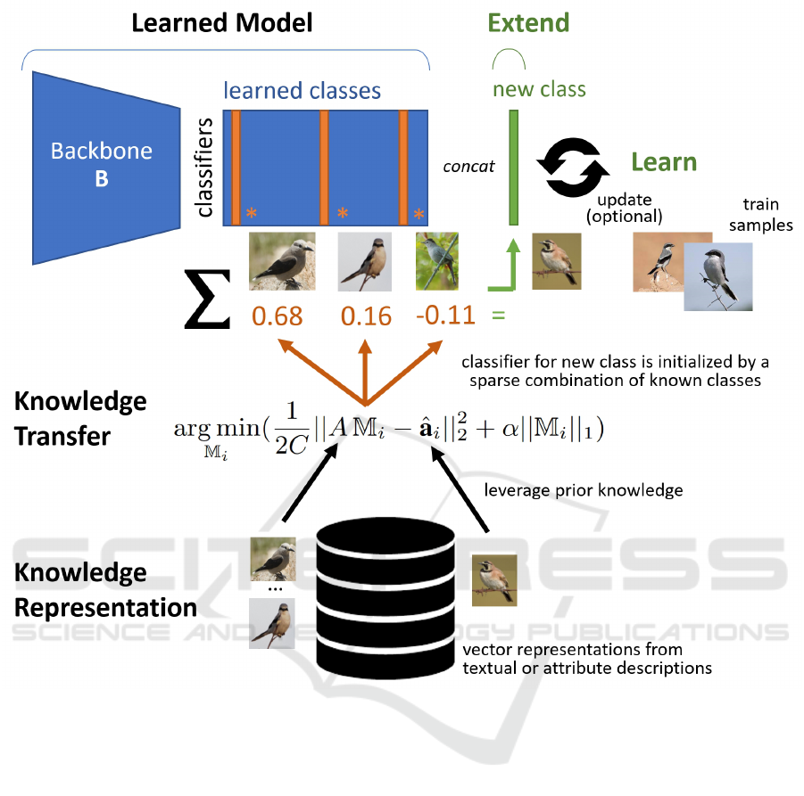
Figure 1: Synthesizing classifiers for a new class from known classes, by recombining the neural classifier weights (column
vectors) via a sparse linear mapping. The mapping is determined from prior knowledge. The synthesized classifier for a new
class is useful for zero-shot recognition and provide a kickstart for few-shot learning.
et al., 2022b; Zhou et al., 2022a), or unified tokens
(Zang et al., 2023). For instance, CoOp (Zhou et al.,
2022b) is modeling the context of CLIP prompts as
a set of learnable tokens, instead of manually tun-
ing the prompt. This is very effective and achieves
state-of-the-art results on several benchmarks (Zhou
et al., 2022b). However, there are two important
drawbacks of prompt learning. Firstly, it can only be
done for language-vision models, whereas we aim for
a method that can work for various types of neural
networks. Secondly, the learned prompts are vectors
that lack an explicit meaning, which makes it hard
to interpret them. The representation of the new class
cannot be checked by its relation to the known classes.
In our paper, we will visualize the new class by how
it was mapped explicitly from the known classes with
their respective weights. Interestingly, we find that it
is essential to not limit this mapping to the most sim-
ilar known classes, but dissimilar classes (with neg-
ative weights) are also necessary to reflect properties
that are absent in the new class. Another drawback of
prompt learning is that explicit prior knowledge about
the known classes and new class is not taken into ac-
count in the process of learning the new class. In our
paper, we leverage various types of knowledge repre-
sentations.
A recent line of research is to improve the fea-
tures such that they better transfer to new classes
within a specific domain. For example, the fine-
grained feature composition framework that learns to
extract very powerful attribute features that are both
selective and diverse (Huynh and Elhamifar, 2021).
They show very good performance on classifying new
classes of birds, by learning good, transferable fea-
Synthesizing Classifiers from Prior Knowledge
49

tures. Such feature learning approaches are orthog-
onal to our method. They focus on better features,
which is indeed key for better classification as demon-
strated by reporting the best performance on several
zero-shot datasets. To the contrary, we focus on better
reuse of the classifier head of a given model. A better
model as a starting point will improve the synthesized
classifiers that can be derived thereof, as we will show
for the popular CLIP model (Radford et al., 2021)
which provides strong features (Zhou et al., 2022b;
Zhou et al., 2022a).
3 METHOD
We synthesize classifiers from known classes, by re-
combining the weights from the classification head
on known classes. This recombination is performed
by a linear, sparse reconstruction. Sparsity is a de-
sign choice to mitigate overfitting. The reconstruc-
tion is derived from auxiliary information, including
attributes and language embeddings of class labels or
textual descriptions. In this way, we synthesize the
classifier head for the new classes, where the back-
bone is initially copied from the model on the known
classes. This backbone can be adopted from a pre-
trained model (e.g. on Imagenet) or finetuned on
known classes. The backbone can be a specialized
one that captures the specific features that are dis-
criminative for the classes of interest, such as the fine-
grained feature composition framework from (Huynh
and Elhamifar, 2021). After synthesizing our classi-
fiers, they operate in a zero-shot manner. Given that
the synthesized classifiers are standard tensors, they
can be optimized further using a few labeled samples
of the new classes, including the classification head
and optionally the backbone if desired. Because the
synthesized classifiers have weights that are approxi-
mately correct, they provide an excellent start for few-
shot learning on the new classes.
3.1 Problem Definition
The zero-shot learning task can be formalized as min-
imization of the regularized empirical risk (Xian et al.,
2018) and involves classes for which there are labeled
samples (known classes) and new classes without la-
bels;
1
N
N
∑
n=1
L(y
n
, h(x
n
;W )) + Ω(W ) (1)
where h: X → Y is a classifier with parameters W .
The classifier learns to classify samples x
n
into re-
spective classes y
n
for a training set S = {(x
n
, y
n
), n =
1. . . N} with y
n
∈ Y
known
. Here, L is the loss function
and Ω(·) the regularization term. At test time, the
goal is to correctly classify samples of unseen, new
classes, Y
new
, with Y
new
∩ Y
known
=
/
0. We assume L
to be the cross-entropy loss.
3.2 Synthesizing Classifiers
The objective is to transform the function h(·;W ),
which is trained on the known classes, into a new
function
ˆ
h(·;
ˆ
W ) that can classify samples into the new
classes. The function h(·) is a neural network that
transforms a sample x
i
into class logits o
i
= h(x
i
;W ) ∈
R
C
, where C is the number of known classes, |Y
known
|.
The outputs o
i
serve as input for a softmax activa-
tion followed by a cross-entropy loss. We decompose
h(x
i
;W ) as:
h(x
i
) = g( f (x
i
;W
f
);W
g
) (2)
where f (·) ∈ R
D
is a feature extractor (i.e., the back-
bone of a neural network) to yield a D-dimensional
feature vector and g(·) ∈ R
C
is the classifier head per-
forming an operation from R
D
→ R
C
. The feature ex-
tractor f (·) can be pretrained on another dataset (e.g.,
a Resnet on Imagenet (He et al., 2016)) or trained or
finetuned on the training set of known classes, S . We
assume g(·;W
g
) to be a linear classifier, so W
g
con-
sists of a weights matrix w ∈ R
D×C
and a bias vector
b ∈ R
C
.
Given the neural network trained on the known
classes, h(x
i
;W ) = g( f (x
i
;W
f
);W
g
) ∈ R
C
, we derive
ˆ
h(·) ∈ R
ˆ
C
to classify samples into the new classes
(
ˆ
C = |Y
new
|). To obtain
ˆ
h(·), we transform g(·) into
ˆg(·):
ˆ
h(x
i
) = ˆg( f (x
i
;W
f
);W
ˆg
) ∈ R
ˆ
C
(3)
Note that f (·;W
f
) remains unchanged.
We transform g(·;W
g
) into ˆg(·;W
ˆg
), by transform-
ing its parameters: W
g
→ W
ˆg
. Similar to g(·;W
g
), W
ˆg
consists of a weights matrix ˆw ∈ R
D×
ˆ
C
and a bias vec-
tor
ˆ
b ∈ R
ˆ
C
, but now projecting to
ˆ
C (new classes)
instead of C (known classes). We transform w → ˆw
and b →
ˆ
b to construct W
ˆg
for synthesizing ˆg(·;W
ˆg
)
thereby acquiring the desired
ˆ
h(·) from Equation 3.
For w → ˆw, we synthesize ˆw = w · M as an dot prod-
uct in Euclidean space between the classifier weights
w and a coupling matrix M ∈ R
C×
ˆ
C
. M is detailed
in Section 3.3. Similarly, for b →
ˆ
b, we synthesize
ˆ
b = b · M as a dot product between the classifier bias
and the same coupling matrix M.
VISAPP 2024 - 19th International Conference on Computer Vision Theory and Applications
50

After synthesizing
ˆ
h(·), the obtained zero-shot
classifier can be finetuned further on the new classes
once a few labels are available, by straightforward
learning with the cross-entropy loss. Optionally
this includes finetuning of the model’s backbone
f (·;W
f
) →
ˆ
f (·;W
ˆ
f
).
3.3 Knowledge Transfer
The coupling matrix M is the key ingredient for syn-
thesizing the classifiers for the new classes from the
classifiers for the known classes. M is derived us-
ing auxiliary, semantic information about the known
and new classes. Common auxiliary sources are at-
tributes and language embeddings of the class labels
(Xian et al., 2018). For our classifier synthesis, it is
essential that M is the result of a robust derivation
that generalizes well. We need at least one auxiliary
vector per class to derive M. In practice, there often
is one auxiliary vector per class, which is very lim-
ited to derive M robustly. We consider it a risk that
the derivation is overfitted by including many classes
with very small weights. To mitigate this risk, we
consider sparse, linear estimation of M. Auxiliary
vectors are assumed to be available for the known
classes {(Y
i
, a
i
), Y
i
∈ Y
known
} and for the new classes
{(
ˆ
Y
i
,
ˆ
a
i
),
ˆ
Y
i
∈Y
new
}, where a
i
is a vector that describes
class Y
i
. M ∈ R
C×
ˆ
C
is constructed column-wise, by it-
erating over each new class
ˆ
Y
i
, which corresponds to
column vector i of M and denoted by M
i
. The deriva-
tion of M
i
is based on a Lasso formulation (Tibshi-
rani, 1996) and yields a sparse, linear estimation given
the known classes:
argmin
M
i
(
1
2C
||AM
i
−
ˆ
a
i
||
2
2
+ α||M
i
||
1
) (4)
where C is the number of known classes and A is the
matrix that consists of stacked auxiliary vectors for
the known classes, i.e., {a
i
}. The resulting estimate
solves the minimization of the least-squares error with
a L
1
regularization term on the coefficients M
i
to pre-
fer solutions with fewer non-zero coefficients. The
degree of regularization is steered by α. This is im-
portant to reduce the number of known classes upon
which the estimate is dependent, in order to avoid
overfitting of the new classes that are to be estimated.
We consider an implementation of (sklearn, 2023)
that uses coordinate descent to fit the coefficients. Hy-
perparameter α is set in the experiments. Fortunately,
we found that one value is good for the various exper-
iments with different datasets, which indicates that it
can be robustly set without severe tuning.
4 EXPERIMENTS
In the experiments, we validate whether our synthe-
sized classifiers are indeed useful for zero-shot recog-
nition and whether they provide a good starting point
for few-shot learning. We will compare with strong
baselines that require either costly annotation of at-
tributes (e.g., ALE (Akata et al., 2015a)) or heavy
pretraining (CLIP (Radford et al., 2021)). Of par-
ticular interest is classification of finegrained classes
(because the visual differences are small) and uncom-
mon classes (because zero or only a few images will
be available in practice). In the following subsections,
we assess our method for respectively zero-shot fine-
grained classification, few-shot finegrained classifica-
tion, a known hard case from zero to few shots, and
uncommon finegrained classes. The experiments can
be replicated from code which is availabe.
4.1 Zero-Shot Finegrained
Classification
4.1.1 Setup
For finegrained classification, we consider a dataset of
images of 200 bird species, i.e. CUB-200 (Wah et al.,
2011). The birds are distinguished by 312 attributes.
We follow the standard setup from (Xian et al., 2018),
where 50 new classes are held out for evaluation of
zero-shot classification. Following (Xian et al., 2018)
we use the provided attributes per class (a vector) and
the features per image (a vector) that were extracted
from a Resnet-101 model (He et al., 2016) pretrained
on Imagenet (Deng et al., 2009), i.e., f (·) in Equa-
tions 2 and 3. On the known classes, we learn the
classifier on the image features. Using the attribute
vectors, we derive the mapping M (Equation 4) from
the known classes to the 50 new classes, with α = 1e-
5. With the mapping M, we transform the classifier
weights for the known classes to obtain the synthe-
sized classifiers for the 50 new classes.
4.1.2 Results
Our method achieves an accuracy of 0.540, which is
almost on-par with the best performer in (Xian et al.,
2018), ALE (Akata et al., 2015a), which achieves
an accuracy of 0.549 (Table 1). Both methods (top
two rows in Table 1) use attributes as auxiliary in-
formation, hence both are not efficient because they
require n
classes
× n
attributes
annotations (for CUB-200
this becomes 200 × 312 = 62, 400 annotations). The
ALE model is trained with the attributes, whereas the
base classifiers in our model are trained with class in-
Synthesizing Classifiers from Prior Knowledge
51

Table 1: Our method is almost on-par with a good performer (ALE) on zero-shot learning on CUB200, with the additional
benefits of being extendable to more attributes, handling efficient auxiliary sources at a small drop in accuracy, and kickstarting
few-shot learning.
Method Classifier Exten- Prior Effi- Coupling Kick- Acc.
dable? knowledge cient? starter?
ALE Attributes ✗ Attributes ✗ Bilinear ✗ 0.549
Synthesized Class labels ✓ Attributes ✗ Lasso ✓ 0.540
Synthesized Class labels ✓ Class descriptions ✓ Lasso ✓ 0.459
Synthesized Class labels ✓ Class labels ✓ Lasso ✓ 0.440
dices only, which may cause that ALE performs bet-
ter. Our synthesized classifiers can efficiently deal
with new attributes whenever they become available,
as they are only used a-posteriori, i.e., after learning
the base classifiers, for coupling the known to new
classes. Contrary, when new attributes become avail-
able, attribute models such as ALE require additional
annotation and retraining. Furthermore, in the next
subsection we will show that our synthesized classi-
fiers bring the additional advantage that they serve as
a starting point for few-shot learning.
Figure 2 shows the 50 classes, ordered by the
accuracy achieved by our method, with top-left the
most accurate class and bottom-right the least accu-
rate class. The birds are photographed in challenging
conditions, where they are partially visible, in very
different poses and surrounded by clutter.
4.1.3 Visualizations
Figure 3 shows how our method synthesizes new
classes from the known classes. Note that the amount
of known classes for the estimation of a new class can
differ for various new classes. For instance, the clas-
sifier for Loggerhead Shrike is constructed from com-
bining three classifiers from respectively the Great
Grey Shrike (0.68), Cark Nutcracker (0.16) and Gray
Catbird (-0.11).
These weights come from M
i
in Equation 4. A
negative weight means that the known class is consid-
ered to be negatively correlated with the new class.
Indeed, the new class mostly looks like the known
classes that were assigned positive weights, and dif-
ferent from the ones that were assigned negative
weights.
4.1.4 Other Knowledge Representations
In addition, we assess how much performance is lost
when there are no attribute annotations available. An-
notating attributes is very costly, especially for the
birds which for the CUB-200 dataset have 312 at-
tributes. We defer to other sources of prior informa-
tion, i.e., the labels of the classes or textual descrip-
tions of the classes. These descriptions embedded by
the text encoder of CLIP, but it can be any other text
encoder of a language model. The class labels are pro-
vided by the dataset, whereas the textual description
of the classes are obtained from ChatGPT (OpenAI,
2023). These descriptions are provided in the Ap-
pendix 5.1 and with the code that is made available.
For this experiment, we replace the attribute vectors
by the language embedding vectors of the class de-
scription or class label. These embeddings are gener-
ated by feeding each class description through CLIP’s
language embedder (Radford et al., 2021). Without
any attributes, Table 1 third row, our method yields
an accuracy of 0.459 (-0.081), whereas feeding the
class labels to CLIP (fourth row) yields an accuracy
of 0.440 (-0.100). A reasonable result can be obtained
without the costly attributes.
4.2 Few-Shot Finegrained Classification
4.2.1 Setup
Our synthesized classifiers can be optimized further
for the new classes when some labeled images are
available, i.e., finetuning
ˆ
h(·) from Equation 3. We
are interested in learning with 1 to 4 labels per class.
To finetune
ˆ
h(·), we train only the classifier layer ˆg(·),
because the features
ˆ
f (·) = f (·) are provided by the
benchmark as-is (Resnet101). For completeness, we
also compare with CLIP (Radford et al., 2021) image
encoder, which is a transformer architecture. This is
to show the flexibility of our method for the two main
neural network architectures for image classification
(convolutional neural networks and transformer mod-
els). Recall that ˆg(·) is a single linear layer, for which
we use the rectified Adam optimizer (Liu et al., 2020)
with a batch size of 8 images, a learning rate of 1e-5,
no regularization (Ω in Equation 1) and early stop-
ping on plateau. The labels are randomly drawn. We
repeat the experiment three times for each method and
for each amount of labels per class.
4.2.2 Results
Figure 4 shows that the synthesized classifiers are an
excellent starting point for few-shot learning, because
their weights are already roughly good when initial-
ized from known classes. Figure 4a shows indeed that
VISAPP 2024 - 19th International Conference on Computer Vision Theory and Applications
52

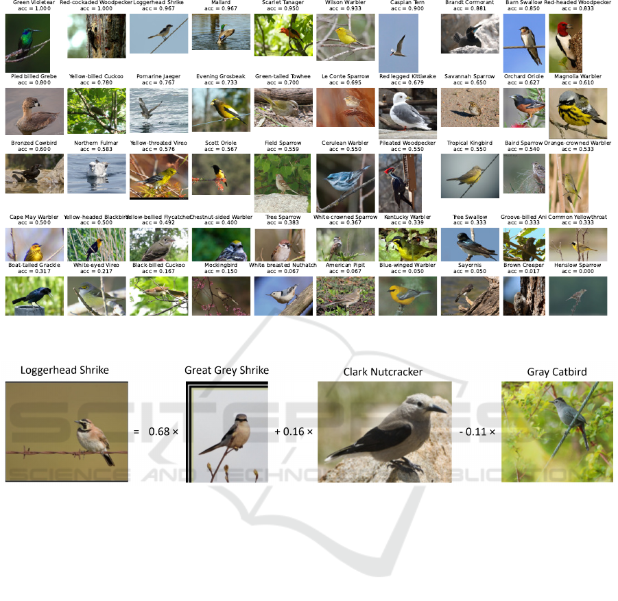
Figure 2: The new classes and the zero-shot accuracy achieved by our synthesized classifiers from known classes, using
attributes as auxiliary information.
Figure 3: Synthesizing a new class (left column) from known classes (other columns), i.e., M
i
in Equation 4, using attributes
as auxiliary information.
our initialization is much better than the conventional
random initialization. Interestingly, with only one la-
bel per class, a significant gain is achieved already,
improving beyond ALE.
For zero-shot modeling, CLIP (Radford et al.,
2021) is a very strong baseline. Indeed, for the zero-
shot case, it outperforms ALE and our method by
a large margin: 0.71 versus 0.55. We are curious
whether our method can have benefits beyond CLIP.
Using CLIP’s image embeddings instead of Resnet-
101 embeddings, we can improve on CLIP’s result
with as few as one label per class: +5% absolute com-
pared to CLIP’s zero-shot performance. It is known
that it is not trivial to improve CLIP with only few
labeled images, sometimes even leading to a lower
performance (Zhou et al., 2022b; Zhou et al., 2022a).
For both image features, our synthesized classi-
fiers (Figure 4, red lines) outperform conventional
random initialization of the classifier head (dashed
blue lines). In conclusion, our synthesized classifiers
are an excellent starting point for few-shot learning.
4.3 Hard Case from Zero to Few Shots
4.3.1 Setup
We have performed additional experiments on two ad-
ditional datasets. The first dataset is Animals with
Attributes 2 (AWA2) (Lampert et al., 2013), a dataset
with 50 classes of animals. The second dataset is SUN
(Patterson and Hays, 2012), a dataset with 717 classes
of natural scenes. The SUN dataset is of special inter-
est because recent methods had difficulties to outper-
form the zero-shot results with 1 or 2 labels per class.
This transition is the focus of this paper, therefore we
evaluate our method on this hard case.
4.3.2 Results
On the AWA2 dataset, ALE (Akata et al., 2015a)
reports an accuracy of 59.9%, where our zero-shot
Synthesizing Classifiers from Prior Knowledge
53

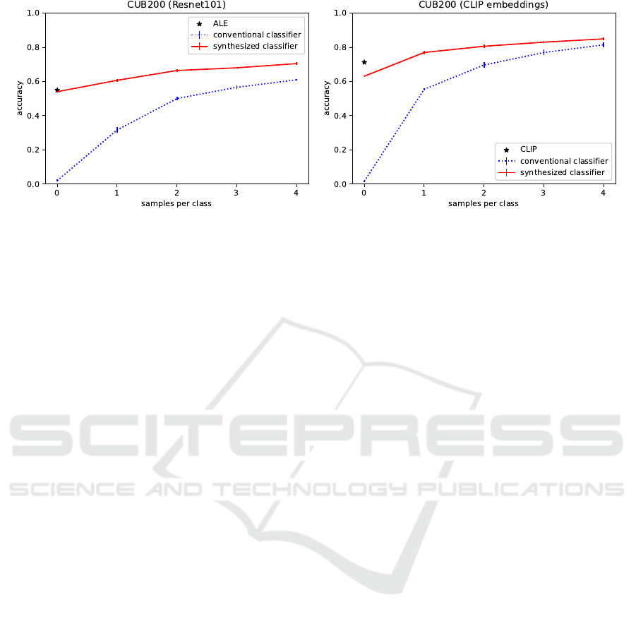
(a) (b)
Figure 4: The synthesized classifiers offers a kickstart for learning new classes with a few labeled images. These synthesized
classifiers are estimated with attributes as auxiliary information. With only one labeled image per class, our method outper-
forms ALE (Akata et al., 2015a) and CLIP (Radford et al., 2021) (star symbols) and conventional random initialization of the
classifier head.
result is 57.1% which increases with 1 label/class:
71.1%. With 2 labels/class, this improves to 78.2%.
Our result is due to the classifier synthesis; without
this initialization the accuracy drops to 70.7% (-7.5).
The same trend is observed for the SUN dataset. ALE
(Akata et al., 2015a) reports and accuracy of 58.1%.
Our result is 55.9% which increases with 1 label/class
to 60.0%. Without our initialization, the accuracy is
only 40% (-20). With 2 labels/class this is improved
further to 63.7% (without our initialization 55.1%).
In conclusion, without our initialization, i.e. conven-
tional classifier training, it is not possible to improve
on the zero-shot results even with 2 labels/class. With
our initialization, steady improvements are achieved.
This is notable, because in (Zhou et al., 2022b) it is
shown that accuracy degrades with more labels: with
1 label/class an accuracy of 61% is reported, whereas
with 2 labels/class the accuracy drops to 59%.
4.4 Uncommon Finegrained Classes
4.4.1 Setup
It is interesting to establish how well our synthesized
classifiers perform on classes that are very uncom-
mon. We know that CLIP’s image embeddings are
strong features for a wide variety of classes (Radford
et al., 2021), also confirmed for birds. This is be-
cause of CLIP’s pretraining on huge collections of
image-text pairs. It may very well be the case that
bird images are part of the pretraining, also hinted by
CLIP’s strong zero-shot performance on the 50 new
bird classes. This is our motivation to look into un-
common classes, to validate whether CLIP may per-
form less on such classes, and how our synthesized
classifiers behave. For this purpose, we collected 850
images of 13 types of military vehicles from web im-
ages. We expect that CLIP has minimal knowledge
about military vehicles, which makes it an interesting
test case. Again this is a fine-grained task, since the
vehicles are very similar in many aspects.
There are no attributes available for the vehicle
classes, which makes it impossible to apply methods
such as ALE. We validate CLIP and our method. In-
stead of an attribute vector per class, we use language
embeddings of the classes. We experiment with the
class labels (name of the vehicle) and the textual de-
scriptions of the classes as obtained from ChatGPT
(OpenAI, 2023). Again, we use CLIP’s text embedder
(Radford et al., 2021) to acquire the auxiliary vectors.
The class descriptions are provided in the Appendix
5.2.
We validate how well the images can be ranked ac-
cording to a particular class of interest (query), mea-
sured by area-under-the-curve (AUC). For this pur-
pose, we take one class as a query and withhold it
from the learning process. All other 12 remaining
classes are the known classes for learning the model
h(·) (Equation 2) that is used for synthesizing clas-
sifiers
ˆ
h(·) (Equation 3) for zero-shot recognition.
This procedure is repeated for all classes. Similar to
the previous experiments, we train only the classifier
layer g(·), with the same training procedure and pa-
rameters.
4.4.2 Results
Figure 6 shows the classes, ordered by the respective
performance achieved by our synthesized classifiers.
For all classes a good performance is realized, except
VISAPP 2024 - 19th International Conference on Computer Vision Theory and Applications
54

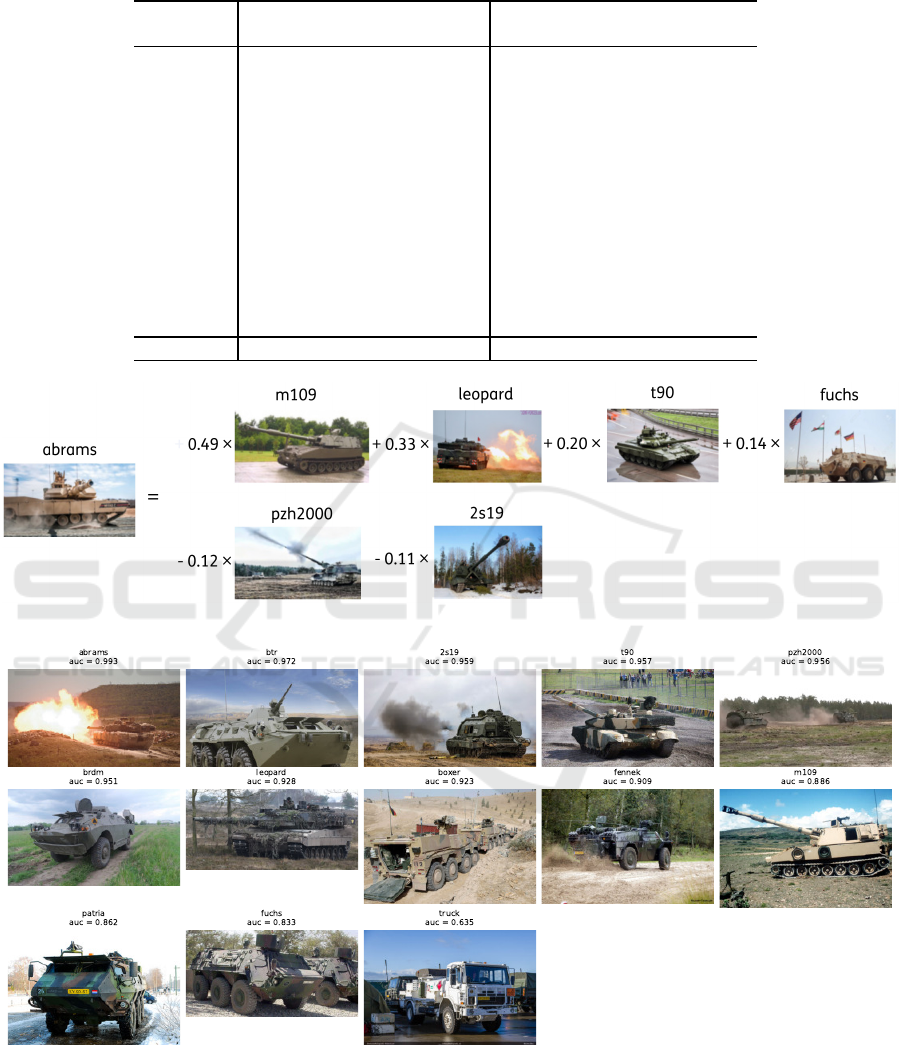
Table 2: Our method often performs better than CLIP on the new, uncommon classes of military vehicles (AUC).
class labels class descriptions
class CLIP ours (gain) CLIP ours (gain)
boxer 0.285 0.829 0.544 0.700 0.923 0.222
fennek 0.573 0.804 0.231 0.749 0.909 0.159
fuchs 0.359 0.805 0.446 0.740 0.833 0.093
btr 0.520 0.960 0.440 0.900 0.972 0.073
brdm 0.853 0.421 -0.432 0.889 0.951 0.062
pzh2000 0.600 0.726 0.126 0.905 0.956 0.052
leopard 0.860 0.819 -0.401 0.899 0.928 0.029
2s19 0.752 0.833 0.081 0.937 0.959 0.022
patria 0.660 0.770 0.110 0.846 0.862 0.017
m109 0.767 0.759 -0.008 0.874 0.886 0.012
t90 0.751 0.869 0.138 0.947 0.957 0.010
abrams
0.975 0.909 -0.066 0.989 0.993 0.004
truck 0.969 0.698 -0.271 0.954 0.635 -0.320
average 0.686 0.785 0.099 0.871 0.905 0.034
Figure 5: Synthesizing a new class (left column) from known classes (other columns), i.e., M
i
in Equation 4.
Figure 6: The new classes and the zero-shot retrieval accuracy (AUC) achieved by our synthesized classifiers from the known
classes (i.e., all other classes).
for the class ‘truck’. The reason is that there are no
other truck-like vehicles in this dataset. It becomes
impossible to make a good synthesized classifier from
the known but unrelated classes. Table 2 shows the
classes and the gain achieved by our method com-
pared to CLIP. For all classes except truck (see ex-
planation above), a gain is observed.
Synthesizing Classifiers from Prior Knowledge
55

4.4.3 Visualizations
Figure 5 shows a coupling from known classes to
a new class that creates the synthesized classifiers.
Likewise the bird classes, the new class mostly looks
like the known classes that were assigned positive
weights (e.g., also tank-like vehicles), and different
from the ones that were assigned negative weights
(e.g., no barrel in front or manufactured in a differ-
ent country).
5 CONCLUSIONS
We have proposed a method that naturally ties zero-
and few-shot learning together, by synthesizing zero-
shot classifiers for new classes from classifiers from
known classes, with the option to optimize the clas-
sifiers further if a few labeled images are available.
We learned that the established classifiers are trans-
parent: their synthesis is based on a mapping that
can be visualized, which provides insights in which
known classes are used to synthesize the new classes.
The synthesis is simple and effective. We found that
it can outperform CLIP, which is a strong baseline. It
leads to better learning with as few as 1-4 training im-
ages, due to the improved starting point. Future work
includes diffusion models to derive the mapping for
synthesizing classifiers.
ACKNOWLEDGEMENTS
This material is based on research sponsored by Air
Force Research Laboratory (AFRL) under agreement
number FA8750-19-C-0514. The U.S. Government
is authorized to reproduce and distribute reprints for
Government purposes notwithstanding any copyright
notation therein. The views and conclusions con-
tained herein are those of the authors and should not
be interpreted as necessarily representing the official
policies or endorsements, either expressed or implied,
of Air Force Laboratory, DARPA or the U.S. Govern-
ment. The other sponsor is EDF: project 101103386
part of EDF-2021-DIGIT-R-2.
REFERENCES
Akata, Z., Perronnin, F., Harchaoui, Z., and Schmid, C.
(2015a). Label-embedding for image classification.
IEEE transactions on pattern analysis and machine
intelligence, 38(7):1425–1438.
Akata, Z., Reed, S., Walter, D., Lee, H., and Schiele,
B. (2015b). Evaluation of output embeddings for
fine-grained image classification. In Proceedings of
the IEEE conference on computer vision and pattern
recognition, pages 2927–2936.
Changpinyo, S., Chao, W.-L., Gong, B., and Sha, F. (2016).
Synthesized classifiers for zero-shot learning. In Pro-
ceedings of the IEEE conference on computer vision
and pattern recognition, pages 5327–5336.
Deng, J., Dong, W., Socher, R., Li, L.-J., Li, K., and Fei-
Fei, L. (2009). Imagenet: A large-scale hierarchical
image database. In 2009 IEEE conference on com-
puter vision and pattern recognition, pages 248–255.
IEEE.
Frome, A., Corrado, G. S., Shlens, J., Bengio, S., Dean,
J., Ranzato, M., and Mikolov, T. (2013). Devise: A
deep visual-semantic embedding model. Advances in
neural information processing systems, 26.
He, K., Zhang, X., Ren, S., and Sun, J. (2016). Deep resid-
ual learning for image recognition. In Proceedings of
the IEEE conference on computer vision and pattern
recognition, pages 770–778.
Huynh, D. and Elhamifar, E. (2021). Compositional
fine-grained low-shot learning. arXiv preprint
arXiv:2105.10438.
Jia, M., Tang, L., Chen, B.-C., Cardie, C., Belongie, S.,
Hariharan, B., and Lim, S.-N. (2022). Visual prompt
tuning. In European Conference on Computer Vision,
pages 709–727. Springer.
Lampert, C. H., Nickisch, H., and Harmeling, S. (2013).
Attribute-based classification for zero-shot visual ob-
ject categorization. IEEE transactions on pattern
analysis and machine intelligence, 36(3):453–465.
Liu, L., Jiang, H., He, P., Chen, W., Liu, X., Gao, J., and
Han, J. (2020). On the variance of the adaptive learn-
ing rate and beyond. In International Conference on
Learning Representations.
OpenAI (2023). ChatGPT. Accessed: 2023-04-21.
Parnami, A. and Lee, M. (2022). Learning from few exam-
ples: A summary of approaches to few-shot learning.
arXiv preprint arXiv:2203.04291.
Patterson, G. and Hays, J. (2012). Sun attribute database:
Discovering, annotating, and recognizing scene at-
tributes. In 2012 IEEE conference on computer vision
and pattern recognition, pages 2751–2758. IEEE.
Pourpanah, F., Abdar, M., Luo, Y., Zhou, X., Wang, R.,
Lim, C. P., Wang, X.-Z., and Wu, Q. J. (2022). A re-
view of generalized zero-shot learning methods. IEEE
transactions on pattern analysis and machine intelli-
gence.
Radford, A., Kim, J. W., Hallacy, C., Ramesh, A., Goh, G.,
Agarwal, S., Sastry, G., Askell, A., Mishkin, P., Clark,
J., et al. (2021). Learning transferable visual models
from natural language supervision. In International
Conference on Machine Learning, pages 8748–8763.
PMLR.
Romera-Paredes, B. and Torr, P. (2015). An embarrassingly
simple approach to zero-shot learning. In Interna-
tional conference on machine learning, pages 2152–
2161. PMLR.
VISAPP 2024 - 19th International Conference on Computer Vision Theory and Applications
56

sklearn (2023). Lasso. Accessed: 2023-04-21.
Socher, R., Ganjoo, M., Manning, C. D., and Ng, A. (2013).
Zero-shot learning through cross-modal transfer. Ad-
vances in neural information processing systems, 26.
Tibshirani, R. (1996). Regression shrinkage and selection
via the lasso. Journal of the Royal Statistical Society:
Series B (Methodological), 58(1):267–288.
Wah, C., Branson, S., Welinder, P., Perona, P., and Be-
longie, S. (2011). The caltech-ucsd birds-200-2011
dataset.
Xian, Y., Akata, Z., Sharma, G., Nguyen, Q., Hein, M., and
Schiele, B. (2016). Latent embeddings for zero-shot
classification. In Proceedings of the IEEE conference
on computer vision and pattern recognition, pages 69–
77.
Xian, Y., Lampert, C. H., Schiele, B., and Akata, Z.
(2018). Zero-shot learning—a comprehensive eval-
uation of the good, the bad and the ugly. IEEE trans-
actions on pattern analysis and machine intelligence,
41(9):2251–2265.
Zang, Y., Li, W., Zhou, K., Huang, C., and Loy, C. C.
(2023). Unified vision and language prompt learning.
arXiv preprint arXiv:2210.07225.
Zhang, Z. and Saligrama, V. (2015). Zero-shot learning
via semantic similarity embedding. In Proceedings
of the IEEE international conference on computer vi-
sion, pages 4166–4174.
Zhou, K., Yang, J., Loy, C. C., and Liu, Z. (2022a). Con-
ditional prompt learning for vision-language models.
In Proceedings of the IEEE/CVF Conference on Com-
puter Vision and Pattern Recognition, pages 16816–
16825.
Zhou, K., Yang, J., Loy, C. C., and Liu, Z. (2022b). Learn-
ing to prompt for vision-language models. Inter-
national Journal of Computer Vision, 130(9):2337–
2348.
APPENDIX
Bird Descriptions
The class descriptions generated by ChatGPT (Ope-
nAI, 2023):
001.Black footed Albatross Black-footed Alba-
tross: Large with dark plumage and a distinctive
yellow eyering, found in the Pacific Ocean.
002.Laysan Albatross Laysan Albatross: Large
with white plumage and a pink bill, found on the
Hawaiian Islands.
003.Sooty Albatross Sooty Albatross: Dark
plumage with a pale head and neck, found in the
Southern Ocean.
004.Groove billed Ani Groove-billed Ani: Long-
tailed with a distinctive grooved bill and iridescent
plumage, found in scrubland habitats.
005.Crested Auklet Crested Auklet: Small and
striking, with a curly crest and white plumage
with black markings, found in coastal waters.
006.Least Auklet Least Auklet: Tiny and dumpy
with dark plumage and a distinctive white eye,
found in coastal waters.
007.Parakeet Auklet Parakeet Auklet: Brightly col-
ored with a green and orange bill, found in coastal
waters.
008.Rhinoceros Auklet Rhinoceros Auklet: Large
with a distinctive horn-like bill and dark plumage,
found in coastal waters.
009.Brewer Blackbird Brewer Blackbird: Glossy
black with a distinctive pale eye, found in open
habitats and farmland.
010.Red
winged Blackbird Red-winged Blackbird:
Black with red and yellow wing patches and a dis-
tinctive conk-la-ree song, found near water.
011.Rusty Blackbird Rusty Blackbird: Dark with
a rusty-brown head and distinctive yellow eyes,
found in wetland habitats.
012.Yellow headed Blackbird Yellow-headed
Blackbird: Striking with black plumage and a
bright yellow head, found in wetland habitats.
013.Bobolink Bobolink: Striking with black and
white plumage and a distinctive bubbling song,
found in grassland habitats.
014.Indigo Bunting Indigo Bunting: Striking with
deep blue plumage and a distinctive warble song,
found in open woodlands and suburbs.
015.Lazuli Bunting Lazuli Bunting: Bright blue
above with a rusty breast, found in open habitats
near water.
016.Painted Bunting Painted Bunting: Strikingly
colored with blue, green, and red plumage, found
in shrubby habitats.
017.Cardinal Cardinal: Strikingly colored with a
bright red crest and black mask, found in wood-
land habitats and suburbs.
018.Spotted Catbird Spotted Catbird: Dark with
white spots and a distinctive red eye, found in
rainforest habitats.
019.Gray Catbird Gray Catbird: Plain gray with a
distinctive black cap and a mewing song, found in
brushy habitats.
020.Yellow breasted Chat Yellow-breasted Chat:
Striking with yellow breast and bold, dark
markings, found in brushy habitats.
Synthesizing Classifiers from Prior Knowledge
57

021.Eastern Towhee Eastern Towhee: Striking with
black upperparts, rusty sides, and white belly,
found in shrubby habitats and woodlands.
022.Chuck will Widow Chuck-will’s-widow:
Large and plain with a distinctive call, found in
open woodlands and scrubby habitats.
023.Brandt Cormorant Brandt Cormorant: Dark
with a distinctive hooked bill, found in coastal wa-
ters.
024.Red faced Cormorant Red-faced Cormorant:
Dark with a red face and a white flank patch,
found in coastal waters.
025.Pelagic Cormorant Pelagic Cormorant: Dark
with a distinctive white flank patch, found in
coastal waters.
026.Bronzed
Cowbird Bronzed Cowbird: Shiny
black body with iridescent bronze wings, found
in grasslands and open areas.
027.Shiny Cowbird Shiny Cowbird: Black body
with iridescent blue-green head and bronzy wings,
found in open areas and near water.
028.Brown Creeper Brown Creeper: Small bird
with brownish plumage and long, curved bill,
found in wooded areas.
029.American Crow American Crow: Large, all-
black bird with distinct caw call, found across
North America.
030.Fish Crow Fish Crow: Smaller than American
Crow with hoarser voice, found near water.
031.Black billed Cuckoo Black-billed Cuckoo:
Slender bird with brownish plumage and curved
bill, found in wooded areas.
032.Mangrove Cuckoo Mangrove Cuckoo: Brown-
ish bird with curved bill and distinctive call, found
in mangrove swamps.
033.Yellow billed Cuckoo Yellow-billed Cuckoo:
Similar to Black-billed Cuckoo but with yellow
bill, found in wooded areas.
... etc.
Vehicle Descriptions
The class descriptions generated by ChatGPT (Ope-
nAI, 2023):
1: Abrams The M1 Abrams is an American third-
generation main battle tank. It is named after
General Creighton Abrams, former Army Chief
of Staff and commander of US military forces in
Vietnam from 1968 to 1972.
2: Leopard The Leopard is a family of main battle
tanks developed by Germany in the 1960s and
1970s. It is widely regarded as one of the best
tanks in the world.
3: T90 The T-90 is a Russian third-generation main
battle tank that entered service in 1993. It is a
modernized version of the T-72 tank.
4: 2S19 The 2S19 Msta is a Russian self-propelled
howitzer that entered service in 1989. It is one of
the most powerful artillery systems in the world.
5: M109 The M109 is an American self-propelled
howitzer that has been in service since 1963. It
has been widely used by the US Army and many
other countries around the world.
6: PzH 2000 The PzH 2000 is a German self-
propelled howitzer that entered service in 1998.
It is considered one of the most advanced artillery
systems in the world.
7: BRDM The BRDM is a Russian amphibious ar-
mored scout car that entered service in 1962.
It has been used by many countries around the
world.
8: Fennek The Fennek is a Dutch/German recon-
naissance vehicle that entered service in 2003.
It is designed to operate in a variety of environ-
ments, from deserts to snowy mountains.
9: Boxer The Boxer is a German wheeled armored
vehicle that entered service in 2009. It is designed
to be modular and can be easily adapted for a va-
riety of roles.
10: BTR The BTR is a Russian wheeled armored
personnel carrier that has been in service since
1961. It has been widely used by the Soviet Union
and many other countries around the world.
11: Fuchs The Fuchs is a German armored person-
nel carrier that entered service in 1979. It is de-
signed to operate in a variety of environments,
from deserts to snowy mountains.
12: Patria The Patria is a Finnish wheeled armored
vehicle that entered service in 2006. It is designed
to be highly modular and can be easily adapted for
a variety of roles.
13: Truck Military trucks are an essential part of any
military force, used for a variety of tasks including
transportation of troops, supplies, and equipment.
VISAPP 2024 - 19th International Conference on Computer Vision Theory and Applications
58