Tab-VAE: A Novel VAE for Generating Synthetic Tabular Data

Syed Mahir Tazwar

, Max Knobbout

2 a

, Enrique Hortal Quesada

1 b

and Mirela Popa

1 c

Department of Advanced Computing Sciences, Faculty of Science and Engineering, Maastricht University, P.O. Box 616,

6200 MD, Maastricht, The Netherlands

Just Eat Takeaway.com, Amsterdam, The Netherlands

Keywords:

Generative AI, Variational Autoencoders, GANs, Tabular Data Representation.

Abstract:

Variational Autoencoders (VAEs) suffer from a well-known problem of overpruning or posterior collapse due

to strong regularization while working in a sufﬁciently high-dimensional latent space. When VAEs are used

to generate tabular data, categorical one-hot encoded data expand the dimensionality of the feature space

dramatically, making modeling multi-class categorical data challenging. In this paper, we propose Tab-VAE,

a novel VAE-based approach to generate synthetic tabular data that tackles this challenge by introducing

a sampling technique at inference for categorical variables. A detailed review of the current state-of-the-

art models shows that most of the tabular data generation approaches draw methodologies from Generative

Adversarial Networks (GANs) while a simpler more stable VAE method is ignored. Our extensive evaluation

of the Tab-VAE with other leading generative models shows Tab-VAE improves the state-of-the-art VAEs

signiﬁcantly. It also shows that Tab-VAE outperforms the best GAN-based tabular data generators, paving the

way for a powerful and less computationally expensive tabular data generation model.

1 INTRODUCTION

Tabular data is crucial for data-driven industries

across a variety of domains and is essential for many

computationally demanding applications. Analysis of

tabular data can provide valuable insights for com-

panies, but obtaining and sharing real data for anal-

ysis can be difﬁcult due to various factors such as

the cost and difﬁculty of data collection. Addition-

ally, it may not always be feasible to obtain large

enough amounts of high-quality real-world data. To

overcome these challenges, synthetic data generation

methods have been developed. Synthetic data, based

on real data and preserving its statistical properties,

can be used for product testing, model training, and

data retention while ensuring regulatory compliance.

Moreover, synthetic tabular data can be used to sim-

ulate scenarios where real-world data is limited. By

generating diverse synthetic data and combining it

with real data, the robustness and generalization of

machine learning models can be improved in various

industries.

Deep generative models like variational autoen-

https://orcid.org/0009-0006-0918-0441

https://orcid.org/0000-0003-2119-4169

https://orcid.org/0000-0002-6449-1158

coders (VAE) (Kingma and Welling, 2013) and gen-

erative adversarial networks (GAN) (Goodfellow Ian

et al., 2014) have had massive success recently in

modeling and generating synthetic images (Karras

et al., 2019) and texts (Guo et al., 2018). Recent ef-

forts have been made to use deep generative models

to create synthetic tabular data in an attempt to repli-

cate the success seen in other domains (Figueira and

Vaz, 2022). While some methods have been success-

ful, they primarily rely on GANs. The reliance on

GANs may be attributed to their success in generat-

ing images, as reported in (Elasri et al., 2022), since

GANS are typically able to produce clearer images.

Nevertheless, in the context of tabular data, the advan-

tages of VAEs could be more effectively utilized, pri-

marily due to several disadvantages associated with

GANs. Training and evaluating them can be challeng-

ing due to their sensitivity to random initialization and

hyperparameter settings. This often leads to gener-

ators with similar architectures and hyperparameters

behaving differently. GANs also struggle with mode

collapse, where the generator produces samples that

only resemble a few modes of the data distribution.

This is a well-known issue, as reported in the litera-

ture such as (Goodfellow, 2016) and (Salimans et al.,

2016). Evaluating the quality of GANs is also dif-

Tazwar, S., Knobbout, M., Quesada, E. and Popa, M.

Tab-VAE: A Novel VAE for Generating Synthetic Tabular Data.

DOI: 10.5220/0012302400003654

Paper published under CC license (CC BY-NC-ND 4.0)

In Proceedings of the 13th International Conference on Pattern Recognition Applications and Methods (ICPRAM 2024), pages 17-26

ISBN: 978-989-758-684-2; ISSN: 2184-4313

ﬁcult as determining the likelihood is an intractable

problem. The current standard is to qualitatively ex-

amine the samples produced by the generator, but this

provides limited insight into the generator’s coverage

and makes it difﬁcult to understand mode collapse.

This has been reported in the literature such as (Bo-

janowski et al., 2017).

On the other hand, VAEs have a more straightfor-

ward and stable training process. Additionally, VAEs

do not encounter problems such as mode collapse

because their loss function requires them to recon-

struct the entire dataset, making them less sensitive

and more robust. The latent space of a VAE is also

easy to interpret, as it can be inspected by analyzing

events in different regions of the latent space, as re-

ported in the literature such as (Spinner et al., 2018).

Therefore, it seems more practical to use VAEs for

generating representative synthetic tabular data.

It is important to note that there are unique chal-

lenges when modeling tabular data. One such chal-

lenge is the need to model both discrete and continu-

ous columns simultaneously, as well as the presence

of multi-modal non-Gaussian values within each con-

tinuous column and a severe imbalance of categori-

cal columns. Modeling a multi-class categorical col-

umn is particularly challenging for VAEs due to is-

sues such as overpruning and information preference

property, as reported in the literature such as (Burda

et al., 2015) and (Zhao et al., 2017). This refers to the

tendency of VAEs to neglect a large number of latent

variables when working in high dimensional latent

space due to strong self-regularization, as reported in

(Asperti, 2018), resulting in sub-optimal generative

models.

To address this challenge in VAEs, we adopt a

technique that uses sampling during inference to ex-

tract suppressed information and properly model the

multi-class categorical variable. By combining the

strengths of deep generative models to overcome the

unique challenges of tabular data synthesis and our

own novel approach to address overpruning, we pro-

pose the Tabular Variational Autoencoder (Tab-VAE).

Tab-VAE encodes various types of tabular data fea-

tures using a custom feature transformer, and then

trains a vanilla VAE-based architecture with custom

input and output layers to model the data and gener-

ate representative synthetic data. Our contribution can

be summarised as follows:

• We propose a novel VAE model called Tab-VAE

that can handle various types of tabular data and

can deal with the aforementioned challenges.

• We extensively evaluate Tab-VAE against several

state-of-the-art baselines and show that Tab-VAE

outperforms both the VAE and GAN baselines.

• Our ﬁndings demonstrate that Tab-VAE is con-

siderably faster to train than the top-performing

GAN baseline. Across all datasets, we observed

an 86.1% decrease in runtime when compared to

its counterpart, indicating that Tab-VAE is a com-

putationally less expensive alternative.

2 RELATED WORK

One of the earliest approaches to generate synthetic

tabular data is to combine attributes from existing data

points to create new, synthetic data points. An exam-

ple of this approach is the Synthetic Minority Over-

sampling Technique (SMOTE) (Chawla et al., 2002).

Another early approach to generating synthetic tabu-

lar data involves using statistical models that create a

multivariate probability distribution over the columns

of a table, treating each column as a random vari-

able. Synthetic data is then generated by sampling

values from this distribution. Examples of methods

that use this approach include CLBN (Chow and Liu,

1968), PrivBayes (Zhang et al., 2017) and copulas

(Patki et al., 2016),(Sun et al., 2019).

Deep learning approaches have also been used to

model the distribution of synthetic tabular data, pri-

marily through the use of GANs (Goodfellow Ian

et al., 2014). MedGAN (Choi et al., 2017) gen-

erates synthetic patient data and can generate high-

dimensional discrete variables, such as binary and

count features, by combining an autoencoder with a

GAN. CorrGAN (Patel et al., 2018) uses the same

architecture as MedGAN but introduces an addi-

tional term in the reconstruction loss of the auto-

encoder to encourage the decoder to preserve the

attributes’ correlation. (Camino et al., 2018) pro-

poses to improve MedGAN architecture by using the

WGAN (Arjovsky et al., 2017) framework with gradi-

ent penalty. It also models multi-categorical discrete

columns. VeeGAN (Srivastava et al., 2017) mitigates

the mode collapse problem in GANs by variational

learning. Table-GAN (Park et al., 2018) adopts the

very famous image generator architecture DCGAN

(Radford et al., 2015) using a convolutional neural

network but has an additional neural classiﬁer that

predicts the label of the synthetic data.

So far, none of the discussed tabular GANs explic-

itly tackle the issue of highly imbalanced categorical

columns and multi-modal continuous columns. CT-

GAN (Xu et al., 2019), using a conditional WGAN-

GP framework introduces Mode-Speciﬁc Normal-

ization (MSN) for modeling multi-modal continu-

ous data, subsequently addressing mode-collapse in

GANs. It also addresses the imbalanced category is-

ICPRAM 2024 - 13th International Conference on Pattern Recognition Applications and Methods

sue with a new training approach called training by

sampling. In the same paper they introduce a vanilla

VAE-based tabular data synthesizer called TVAE (Xu

et al., 2019). TVAE is the ﬁrst of its kind and

compares favorably against CTGAN and other GAN-

based models in extensive evaluation. The most

recent GAN-based approach is CTAB-GAN (Zhao

et al., 2021) and a subsequent enhancement CTAB-

GAN+ (Zhao et al., 2022). It uses a conditional gen-

erator like the CTGAN and uses a lot of elements

like MSN and training by sampling. But it also en-

hances the modeling by introducing a provision for

mixed and long-tailed data types and by adding two

more loss terms. The authors show that CTAB-GAN+

outperforms other state-of-the-art GAN-based mod-

els comprehensively. Finally, the most recent VAE-

based approach has been OVAE (Harsha and Stanley,

2020). It combines differentiable oblivious decision

trees (DODTs) with VAEs, thereby incorporating a

strong inductive bias for tabular data into VAEs. They

compare the OVAE model against several state-of-

the-art baselines including TVAE and CTGAN, and

show that OVAE compares favorably against the base-

lines on 12 real-world datasets.

Previous research on synthetic tabular data gener-

ation has mainly focused on GANs and lacked the use

of VAE-based deep generative models. Additionally,

existing VAE-based models do not address the issue

of overpruning and do not utilize the full capabilities

of VAEs. Our proposed Tab-VAE model addresses

this issue and represents a signiﬁcant advancement in

VAE-based synthetic tabular data generation.

3 BACKGROUND

Our Tab-VAE model uses the VAE methodology to

model data distribution and is compared with other

deep generative models such as GANs and VAEs. We

will brieﬂy explain these techniques in the following

section.

3.1 Generative Adversarial Network

GANs use an unsupervised learning technique to

identify patterns in input data and generate new sam-

ples that mimic the distribution of the original dataset.

A GAN is composed of two main modules, namely

generator, and discriminator, and it is trained to reach

an equilibrium between the two modules. The gener-

ator G is a neural network that samples a noise vector

z from a prior distribution p

(z) and generates a syn-

thetic data sample G(z;θ

), while θ

are the param-

eters of the network G. The discriminator D is an-

other neural network that takes an input data x sam-

pled from the data distribution p

data

(x) and outputs

a single scalar D(x; θ

), denoting whether the pro-

vided data sample is from the original data or not. The

two networks are trained together in a zero-sum game

shown in equation 1, where the generator tries to cre-

ate data that can fool the discriminator, and the dis-

criminator tries to correctly identify whether a piece

of data is real or synthetic.

min

max

V (D,G) =E

x∼p

data

(x)

[logD(x)]+

z∼p

(z)

[log(1 − D(G(z))) (1)

The training continues until the generator produces

synthetic data that is indistinguishable from real data

and the discriminator can no longer distinguish be-

tween them. This strategy leads to a trained generator

that can generate synthetic data which is very close to

real data making p

data

(x) ∼ p

(z).

3.2 Variational Autoencoder

Autoencoder neural networks consist of two neural

networks: an encoder and a decoder. The encoder

maps the input sequence x to meaningful latent space

z and reconstructs the input through the decoder with

minimal error. VAEs are an extension of normal au-

toencoders that regularize the latent space to follow

a Gaussian distribution p(z), which additionally al-

lows sampling data from the latent space. The ob-

jective is to learn the true posterior p

(z|x), where

θ are the parameters of the network, which can be

learned by using Bayesian inference. However, with-

out any simplifying assumptions on p

(z|x) or p

(z),

the problem is intractable since it requires integration

over all possible values of the unobserved variable

z. The classic solution (Kingma and Welling, 2013)

proposes to use a recognition model q

(z|x) as an ap-

proximation to the true posterior p

(z|x). By jointly

optimizing for θ and φ, the posterior inference prob-

lem becomes tractable. It can be solved by minimiz-

ing the Kullback-leibler (KL)-divergence between the

two terms (the parameters θ and φ have been omitted

for simplicity):

(q(z|x)) ∥ p(z|x)) =

q(z|x)log



q(z|x)

p(z|x)



= E

[logq(z|x)] − E

[log p(x, z)] + log p(x)

= L

ELBO

(x) + log p(x)

(2)

Where:

ELBO

(x) = log p(x) − D

(q(·|x) ∥ p(·|x))

Minimizing the KL-divergence term becomes maxi-

mizing the evidence lower bound L

ELBO

(·). We are

Tab-VAE: A Novel VAE for Generating Synthetic Tabular Data

thus maximizing the log-likelihood of the observed

data while simultaneously minimizing the divergence

of the posterior q(·|x) from p(·|x). Once the VAE is

trained using this learning objective, samples can be

drawn through the learned decoder network to gener-

ate synthetic data.

3.2.1 Limitations of VAE for Tabular Data

An important limitation of VAEs is that they tend

to overprune, also called the property of information

preference. Recall that the ELBO loss is a combina-

tion of log p(x) and −D

(q(z|x) ∥ p(z|x)).

The Gaussian distribution is usually used to model

the conditional distribution (q(z|x)) and the prior dis-

tribution (p(x)). But in light of the loss function, if the

KL-divergence term is to be absolutely minimized it

entails that q(z|x) has to perfectly match p(z|x). This

perfect match can only happen if either q(z|x) doesn’t

require to be Gaussian or q(z|x) must be equivalent

to p(z), which is the unit Gaussian and does not carry

any information about the input sequence x. Anything

other than these two situations will incur a penalty

through the KL-divergence term. Due to strong regu-

larization, the KL-divergence term pushes the condi-

tional distribution towards the unit Gaussian without

carrying any information from x. Due to this phe-

nomenon, VAEs have a tendency not to encode all

the information in the latent space if they can avoid

it, which occurs when the regularization term is too

strong. This issue has been called overpruning in (As-

perti, 2018), posterior collapse in (Guo et al., 2020)

and information preference property in (Zhao et al.,

2017). The main challenge this issue poses while

generating tabular data is in terms of modeling the

categorical columns with multiple imbalanced cate-

gories, n. The categorical columns are normalized us-

ing one-hot-encoding, which creates a sparse matrix

where each category becomes a new variable in an n-

dimensional space. The low-frequency classes carry

very low information, but due to the information pref-

erence property these low information variables get

collapsed and the information gets lost. This makes

modeling the categorical variables with a high num-

ber of categories challenging.

3.3 Gumbel-Softmax Distribution

The Gumbel-softmax distribution was introduced si-

multaneously by two papers (Maddison et al., 2016)

and (Jang et al., 2016). The Gumbel-softmax distribu-

tion is a continuous relaxation of the categorical dis-

tribution, which allows for efﬁcient optimization of

discrete variables in a continuous space. Addition-

ally, a method of sampling from this distribution is

proposed, which we refer to as Gumbel-softmax sam-

pling. Suppose we want to sample from a categori-

cal variable, z with unnormalized class probabilities

,π

,.. .,π

. Gumbel-softmax sampling proceeds in

the following manner:

z = argmax

{

+ logπ

}

Where g

,.. .,g

are i.i.d. samples drawn from

Gumbel(0,1). Since argmax is not differentiable, the

authors propose using softmax instead. By combin-

ing all the ingredients, we generate a k-dimensional

vector y = y

,.. .y

as follows:

exp((logπ

+ g

)/τ)

∑

j=1

exp((logπ

+ g

)/τ)

for i = 1,.. .,k

(3)

Here, τ is a temperature variable to control the soft-

ness or relaxation of y. For lower values of τ, y is

approximately distributed according to π. The proof

is provided that shows that the samples are distributed

according to the softmax probability of the classes in

the appendix. This proof was obtained from an article

by (Adams, 2013).

From equation 3, the use of Gumbel-softmax sam-

pling allows us to draw samples from the probabilistic

distribution of a categorical feature, as opposed to de-

terministically choosing the maximum class. Since

this operation maximizes the class probability of the

samples using the log probability of the unnormalized

classes, it provides minority classes a better chance to

be represented and picked. In the context of overprun-

ing, this makes a huge impact. The strong regular-

ization suppresses low-frequency classes, leading to

information loss in the learned decoder. When sam-

pling from a unit Gaussian and taking the maximum

in a deterministic manner, the maximum class is al-

ways produced, regardless of how small the differ-

ence is with other classes. However, Gumbel-softmax

sampling allows us to sample from these regularized

classes, preserving information that may have been

lost otherwise. Therefore, for all the stated reasons,

we propose to sample using Gumbel-softmax at the

inference step for categorical variables.

4 TABULAR VARIATIONAL

AUTOENCODER

Tab-VAE encodes various types of tabular data fea-

tures by utilizing a custom feature transformer. It then

trains a vanilla VAE architecture with customized in-

put and output layers to model the data distribution.

Synthetic data can then be generated by sampling

from this modeled distribution.

ICPRAM 2024 - 13th International Conference on Pattern Recognition Applications and Methods

4.1 Input Data Transformations

The transformer class of the Tab-VAE transforms the

input data based on its column type and prepares it

for encoding. The tabular data T is encoded variable-

by-variable. We make a distinguishment between cat-

egorical and continuous variables. The table T con-

tains N

continuous columns (C

,.. .,C

) and N

cat-

egorical columns (D

,.. .,D

). Each column is con-

sidered to be a separate random variable, forming a

joint distribution P(C

1:N

). A row denoted r

1, j

,.. .,c

, j

1, j

,.. .,d

, j

) is one observation from

this joint distribution. We employ MSN to handle the

multi-modality of continuous variables, as proposed

in (Xu et al., 2019). MSN ﬁrst estimates the num-

ber of modes, k of each continuous variable, C

ﬁtting a variational Gaussian mixture model (VGM)

(Bishop and Nasrabadi, 2006). This learned Gaus-

sian mixture is speciﬁed as

∑

N (µ

,σ

), where

N is the normal distribution, ω

,µ

and σ

are the

weight, mean and standard deviation of each mode

respectively. Each value, c

of the continuous variable

is then associated and normalized using the normal

distribution of the mode having the highest probabil-

ity: α

−µ

4σ

. Moreover, the mode used is then kept

track by a one-hot-encoding, β

. Finally each contin-

uous value,c

is then represented as a concatenation of

and β

The transformer also has provisions to tackle

some special column types. A column of timestamps

is neither categorical nor continuous. To encode the

timestamps column with its properties intact we con-

sider the cyclical nature of time and use a sine-cosine

transformation of the timestamps to preserve this. The

hour-minute-second portion of the time is converted

into two variables of sine and cosine as follows:

sin

= sin(c

2π

), c

cos

= cos(c

2π

)

The remaining values of a time variable

(month/day/year) are considered as categorical

variables. Additionally, any categorical variable with

only one value is removed to reduce dimensionality.

To encode long-tail distributions effectively, we

adopt the approach from (Zhao et al., 2022). Long-

tail distributions are distributions in which a large

portion of observations are concentrated at the lower

end of the scale. Since VGM has difﬁculty capturing

and encoding values towards the tail, long-tail data

is pre-processed using a logarithmic transformation.

For such variables each value c

is compressed using

lower bound l and replaced with c

log

(

logc

if l > 0

log(c

− l + ε) if l ≤ 0

, where ε > 0 (4)

This transformation makes it easier for VGM to en-

code all values, including the ones in the tail, by com-

pressing and decreasing the distance between the tail

and the bulk data.

Finally, the categorical variables are encoded using

one-hot-encoding γ

. Each row is thus represented as

a (2N

+ N

) - dimensional vector, giving us the ﬁnal

input r

which is then passed to the Encoder (⊕ de-

notes concatenation): r

= α

1, j

⊕ β

1, j

⊕ ··· ⊕ α

, j

⊕

, j

⊕ γ

1, j

⊕ ··· ⊕ γ

, j

4.2 Encoder

The encoder of the Tab-VAE is built to model the con-

ditional distribution q

), where r

denotes the

encoded row of input data from section 4.1 and z

is the latent representation produced by the encoder.

This modeling is done using the reparameterization

trick. The encoder actually produces the parameters

of this distribution, the mean, µ and standard devia-

tion σ using two dense layers. Then z

is modeled.

The architecture of the encoder distribution is as fol-

lows:

= ReLU(Dense(r

))

= ReLU(Dense(x

))

µ = Dense(x

)

σ = exp(Dense(x

))

) ∼ N (µ,diag(σ))

4.3 Decoder

Tab-VAE’s decoder is constructed to model the dis-

tribution p

). The decoder generates α

i, j

and

i, j

for continuous columns and γ

i, j

for the categori-

cal columns. Tab-VAE assumes that each α

i, j

has a

normal distribution (with a column-speciﬁc variance

). It also assumes that β

i, j

and γ

i, j

has categorical

probability mass function. The architecture of the de-

coder distribution is as follows:

= ReLU(Dense(z

))

= ReLU(Dense(x

))

i, j

= tanh(Dense(x

))

i, j

∼ N (

i, j

,δ

)

i, j

∼ GumbelSo f tmax(Dense(x

))

i, j

∼ GumbelSo f tmax(Dense(x

))

) =

∏

i=1

i, j

= α

i, j

)

∏

i=1

i, j

= β

i, j

)

∏

i=1

i, j

= γ

i, j

)

Tab-VAE: A Novel VAE for Generating Synthetic Tabular Data

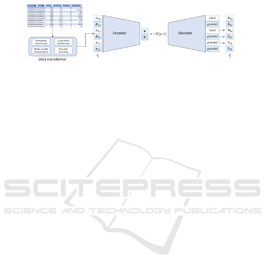
Figure 1: Architectual overview of the Tab-VAE model.

Speciﬁcally,

i, j

is modeled from the continuous por-

tion of the output ˆr

using a tanh activation func-

tion.

i, j

and

i, j

are modeled as a normalized cat-

egorical distribution on the probability simplex us-

ing GumbelSo f tmax activation function. After that,

we simply set the maximum value in each vector to

1, and all other values to 0. This category is cho-

sen as the category of the categorical variable for this

sampled row ˆr

. The parameters of both the encoder

and the decoder are trained by stochastic gradient de-

scent maximizing the evidence lower bound, ELBO

(Kingma and Welling, 2013). The network is trained

using Adam optimizer. The reconstruction loss for

the continuous features, α

i, j

is calculated using mean

squared error. For categorical features γ

i, j

and the

modes β

i, j

, the reconstruction loss is calculated us-

ing cross-entropy loss between the real data and re-

constructed unnormalized class probabilities. For an

overview of the speciﬁc hyperparameters, please refer

to the Appendix.

5 EXPERIMENTS

In this section, we are going to compare Tab-VAE us-

ing two evaluation frameworks. First, we are going

to benchmark it using the ML Efﬁcacy framework

as proposed in (Xu et al., 2019) against the state-

of-the-art baselines discussed in 2, except CTAB-

GAN+. Then we will evaluate Tab-VAE against

CTAB-GAN+ using SDMetrics quality report mea-

suring the synthetic data ﬁdelity(sdm, 2022) and run-

time analysis.

Experiment 1. ML Efﬁcacy. Within the efﬁcacy

framework, we consider several datasets, where every

dataset T is ﬁrst split into T

train

and T

test

. We then

use T

train

to train the model to generate T

syn

of the

same size. T

syn

is used to train a set of standard clas-

siﬁers or regressors and is evaluated with T

test

. The

hyperparameters of these classiﬁers and regressors are

kept the same as the benchmark to enable fair compar-

isons. For regression tasks, the average R

is reported,

while for classiﬁcation tasks metrics like F1, Macro

F1, and accuracy are averaged and reported. The met-

rics are chosen dependent on the dataset following the

benchmark. We also report “Identity”, which simply

trains the classiﬁers and regressors on T

train

instead of

syn

of the real datasets. Identity serves as an upper

bound for all our scores.

The datasets we are using are adopted from (Xu

et al., 2019) to allow for a fair comparison. Par-

ticularly, we consider eight real-world datasets. Six

commonly used machine learning datasets were used:

adult, census, credit, covertype, intrusion and

news from the UCI machine learning repository (Dua

and Graff, 2017), with features and label columns in a

tabular form. Two datasets mnist28 and mnist12 are

obtained by binarizing 28 × 28 and 12 × 12 MNIST

images (LeCun et al., 2010) into feature vectors (with

an additional label column indicating the target digit).

Among these eight datasets one has a continuous vari-

able as its dependent variable, namely news, while the

rest are classiﬁcation datasets.

Our model is compared with several baseline

models discussed in 2. Two of them are Bayesian net-

works, CLBN (Chow and Liu, 1968) and PrivBayes

(Zhang et al., 2017). Four of them are state-of-the-

art GAN models, medGAN (Choi et al., 2017), VEE-

GAN (Srivastava et al., 2017), TableGAN (Park et al.,

2018) and CTGAN (Xu et al., 2019). The remain-

ing two are state-of-the-art VAE models, TVAE (Xu

et al., 2019) and OVAE (Harsha and Stanley, 2020).

The model parameters and other speciﬁcations for the

experiments can be found in the Appendix.

Experiment 2. SDMetrics Fidelity & Runtime. In

the previous experiment, one competing GAN-based

network CTAB-GAN+(Zhao et al., 2022) is missing,

as the authors used a different framework for eval-

uation where they comprehensively showed CTAB-

GAN+ to be the best performing GAN-based tabular

data generator. Nevertheless, to make the evaluation

of Tab-VAE comprehensive, we run experiments to

compare Tab-VAE against CTAB-GAN+. We con-

sider the ﬁdelity of the generated synthetic data and

the computational efﬁciency of the generation process

ICPRAM 2024 - 13th International Conference on Pattern Recognition Applications and Methods

in this comparison.

One approach for evaluating dataset ﬁdelity fo-

cuses on comparing individual column distributions

and correlations between columns. One such method-

ology is called the SDMetrics Quality Score (sdm,

2022). It is part of a broader ecosystem of libraries

dedicated to synthetic data generation called the Syn-

thetic Data Vault (SDV)(Patki et al., 2016). The SDV

project is carried by the DATA to AI Lab team at MIT.

This framework calculates the overall quality scores

along two properties: “Column shapes” and “column

pair trend”. The “column shapes” score measures

how well the synthetic dataset captures the shape of

the distribution of each column. It is calculated using

a metric based on the Kolmogorov-Smirnov statistic

for continuous columns, and a metric based on the to-

tal variation complement for categorical and Boolean

columns. On the other hand “column pair trend”

measures if the synthetic data capture trends between

pairs of columns. It is calculated using Pearson corre-

lation similarity between two continuous columns and

contingency similarity between categorical columns.

For both these properties, a score is given from 0

(worst) to 1 (best). The overall quality score is the

mean score of these two individual scores.

In this experiment, we generate synthetic datasets

based on the same datasets as in the previous ML Ef-

ﬁcacy experiment with the exception of the MNIST

datasets, using both the Tab-VAE and CTAB-GAN+.

We used the provided code base

for generating syn-

thetic datasets using CTAB-GAN+. We report the

SDMetrics quality score. We also report the total

runtime for training these datasets in the competing

models. Both models were trained on Amazon Sage-

maker Studio using ml.g4dn.xlarge, which includes 4

vCPUs, and 1 NVIDIA T4 GPU with 16 GB of GPU

memory.

6 RESULTS

6.1 Experimental Results

Experiment 1. Table 1 shows the detailed results of

the experiments and Table 2 shows the overall result

of the experiments using the ML Efﬁcacy framework.

The boldfaced results indicate the best result and the

underlined ones indicate the second-best result for

each dataset. The values in the Tab-VAE row are from

our experiments, the ones in the OVAE row are ob-

tained from (Harsha and Stanley, 2020), while all the

other results are obtained from (Xu et al., 2019). It

https://github.com/Team-TUD/CTAB-GAN-Plus

is important to note that Tab-VAE beats all the other

models on 4 of the 8 datasets and ties with TVAE on

one dataset. For the remaining three datasets, Tab-

VAE comes second. The three datasets where Tab-

VAE outscores other models by a signiﬁcant margin

are census, covertype, and intrusion. Interest-

ingly, all these three datasets have a signiﬁcant num-

ber of categorical features. This shows Tab-VAE’s

superiority in modeling categorical features. On the

other hand, Tab-VAE comes second with a signiﬁ-

cant margin in the credit dataset which doesn’t have

a single categorical feature except for the target col-

umn. In the MNIST datasets, Tab-VAE comes second

but within a very respectable margin. Overall, Tab-

VAE is the best-performing model on both the classi-

ﬁcation and regression datasets as shown in table 2.

Experiment 2. Table 3 displays the outcomes of the

experiments conducted using SDMetrics Fidelity to

evaluate the synthetic data generated by Tab-VAE and

CTAB-GAN+. The results indicate that Tab-VAE out-

performs CTAB-GAN+ on ﬁve out of the six datasets,

demonstrating the superior ability of our proposed

model to maintain the statistical properties of the orig-

inal datasets. Notably, CTAB-GAN+ also produces

high-quality synthetic data, as reﬂected by its high

quality scores on most datasets. To further investi-

gate the performance of the models, we also com-

pared their runtimes in generating the synthetic data.

Table 4 reports the total runtime of the two mod-

els in generating the datasets. We also included

the dataset dimensions in the table for understand-

ing the reported results. As can be seen from the

table, Tab-VAE generally outperforms CTAB-GAN+

in terms of runtime, with signiﬁcantly faster gener-

ation times observed on all datasets. The runtime

differences are particularly pronounced on datasets

with larger numbers of rows and columns, such as

census, intrusion, and covertype. For instance,

on the census dataset, Tab-VAE runs in 29 minutes,

which is 22 times faster than CTAB-GAN+, which

takes almost 642 minutes (more than 10 hours). One

notable exception is the credit dataset. It exhibits a

smaller difference in runtime between the two mod-

els despite being a very large dataset. This result

can be attributed to the absence of any categorical

columns in the dataset, except for the target column.

This limits the increase in dataset dimensionality fol-

lowing preprocessing. Overall, the results in Table 4

demonstrate that the Tab-VAE algorithm exhibits an

86.1% improvement in total runtime when compared

to CTAB-GAN+. To calculate the total runtime, the

individual runtimes of CTAB-GAN+ and Tab-VAE

are summed across all datasets.

Tab-VAE: A Novel VAE for Generating Synthetic Tabular Data

Table 1: Evaluation of Tab-VAE with other models using the ML Efﬁcacy framework on 8 real-world datasets.

Model adult census credit cover. intru. mnist12 mnist28 news

Macro- Macro- Micro- Micro-

F1 F1 F1 F1 F1 F1 F1 R

Identity 0.67 0.49 0.72 0.65 0.86 0.89 0.92 0.14

CLBN 0.33 0.31 0.40 0.32 0.38 0.74 0.18 -6.28

PrivBayes 0.41 0.12 0.19 0.27 0.38 0.12 0.08 -4.49

medGAN 0.38 0.00 0.00 0.09 0.30 0.09 0.10 -8.80

VEEGAN 0.24 0.09 0.00 0.08 0.26 0.19 0.14 -6.5e6

TableGAN 0.49 0.36 0.18 0.00 0.00 0.10 0.00 -3.09

CTGAN 0.60 0.39 0.67 0.32 0.53 0.39 0.37 -0.43

TVAE 0.63 0.38 0.10 0.43 0.51 0.79 0.79 -0.20

OVAE 0.60 0.38 0.51 0.45 0.53 0.83 0.84 -0.30

Tab-VAE 0.63 0.42 0.61 0.50 0.65 0.81 0.81 0.005

Table 2: Evaluation of Tab-VAE with other models us-

ing ML Efﬁcacy framework averaged over 8 real-world

datasets.

Model Classiﬁcation Regression

Avg. F1 Avg. R

Identity 0.743 0.14

CLBN 0.382 -6.28

PrivBayes 0.225 -4.49

medGAN 0.137 -8.80

VEEGAN 0.143 -6.5e6

TableGAN 0.162 -3.09

CTGAN 0.469 -0.43

TVAE 0.519 -0.20

OVAE 0.591 -0.30

Tab-VAE 0.633 0.005

Table 3: Evaluation of Tab-VAE against CTAB-GAN+ for

synthetic data ﬁdelity using SDMEtrics quality score on 6

real-world datasets.

Dataset CTAB-GAN+ Tab-VAE

adult 90.4% 96.0%

census 84.0% 97.0%

credit 84.6% 97.0%

covertype

98.5% 97.0%

intrusion 68.9% 93.9%

news 94.0% 95.9%

Table 4: Comparison of runtime between CTAB-GAN+ and

Tab-VAE on 6 real-world datasets.

Dataset Dataset properties Runtime in minutes Percentage reduction

Rows Columns CTAB-GAN+ Tab-VAE in runtime

adult 33k 15 19.3 3.4 82.4%

census 300k 41 641.9 29.0 95.5%

credit 284k 30 38.0 20.5 46.3%

covertype 581k 55 372.5 71.8 80.7%

intrusion 494k 41 346.8 65.9 81.0%

news 39k 59 26.6 10.1 62.2%

Total 1731k - 1445.1 200.7 86.1%

Table 5: Ablation analysis for Tab-VAE.

Method adult census credit covertype intrusion

Tab-VAE 0.63 0.42 0.61 0.50 0.65

w/o GS 0.57 0.19 0.00 0.43 0.59

6.2 Impact of Gumbel-Softmax

An ablation analysis was done to check the usefulness

of the novel component Gumbel-softmax for inferring

categorical variables in our model.

Table 5 shows the scores with and without

(“w/o GS”) this component for the ﬁve classiﬁcation

datasets used in the ML Efﬁcacy framework. The

most notable difference can be found in the census

and credit datasets. Interestingly the credit dataset

only has one single categorical column: the target col-

umn. This column only has two classes where one

class accounts for 99.8% of instances and the other

class accounts for only 0.2% of instances, making it

very imbalanced. Because of this huge imbalance,

the synthetic dataset without Gumbel-softmax com-

pletely ignores this minority class, leading to an F1-

score of 0.

On the other hand, among these 5 datasets only

census has more multi-class categorical columns

than continuous columns. Particularly 31 of its 41

columns are multi-class categorical, while 7 of these

columns have more than 30 classes. Inspecting it fur-

ther reveals that most of these columns are imbal-

anced. One example of such a column is ’detailed

household and family stat’, which has 38 classes in

the original dataset. The synthetic dataset generated

by Tab-VAE generates all 38 classes, whereas the one

without Gumbel-softmax generated 34 classes, com-

pletely ignoring/collapsing the information carried by

the other four classes. To illustrate it further, like

credit, census is also a binary classiﬁcation dataset.

The target variable has one class that accounts for

ICPRAM 2024 - 13th International Conference on Pattern Recognition Applications and Methods

93.7% of the instances, making it also highly imbal-

anced. The synthetic dataset generated by Tab-VAE

preserves this ratio whilst the one without Gumbel-

softmax has 97.5% of this class, again suppressing

the information of the minority class. All this fac-

tored into this very low score on the census dataset in

the ablation analysis.

For the remaining three datasets, the performance

difference is not as signiﬁcant, as these datasets

rely less on categorical variables for encoding in-

formation. Interestingly, the adult dataset also has

one multi-class categorical column with 41 classes,

whereas the model without Gumbel-softmax gener-

ates only 9 of these columns. Still, the impact of this

column is not as prevalent as in the case of credit

and census datasets. Similarly to these two datasets,

adult is the only other binary classiﬁcation dataset,

but it has a good ratio of 75%-25% of its two classes.

Therefore, the magnitude of the obtained results high-

lights the importance of Gumbel-softmax in modeling

categorical columns in tabular datasets.

7 CONCLUSIONS AND FUTURE

WORK

In this paper, we introduced Tab-VAE, which ad-

dresses the challenge of modeling multi-class cate-

gorical variables in tabular data using a VAE gener-

ative model. Our approach is motivated by the belief

that VAEs can generate high-quality synthetic data,

with added beneﬁts of being simpler, more stable,

and more computationally efﬁcient. We corroborated

this claim by comparing our model against a host of

state-of-the-art models using two evaluation frame-

works and an ablation analysis. Tab-VAE continu-

ously showed high-level performance across multiple

datasets by outperforming state-of-the-art models of

both GANs and VAEs. In the future, the model can be

made more robust by incorporating additional encod-

ing methods for different types of data, such as mixed

data. Overall, Tab-VAE represents a signiﬁcant ad-

vancement in the ﬁeld of tabular data generation and

has the potential for broad applications in various do-

mains.

REFERENCES

(2022). Synthetic Data Metrics. DataCebo, Inc. Version

0.8.0.

Adams, R. (2013). The gumbel-max trick for discrete distri-

butions — laboratory for intelligent probabilistic sys-

tems.

Arjovsky, M., Chintala, S., and Bottou, L. (2017). Wasser-

stein generative adversarial networks. In Interna-

tional conference on machine learning, pages 214–

223. PMLR.

Asperti, A. (2018). Sparsity in variational autoencoders.

arXiv preprint arXiv:1812.07238.

Bishop, C. M. and Nasrabadi, N. M. (2006). Pattern recog-

nition and machine learning, volume 4. Springer.

Bojanowski, P., Joulin, A., Lopez-Paz, D., and Szlam, A.

(2017). Optimizing the latent space of generative net-

works. arXiv preprint arXiv:1707.05776.

Burda, Y., Grosse, R., and Salakhutdinov, R. (2015).

Importance weighted autoencoders. arXiv preprint

arXiv:1509.00519.

Camino, R., Hammerschmidt, C., and State, R. (2018).

Generating multi-categorical samples with gen-

erative adversarial networks. arXiv preprint

arXiv:1807.01202.

Chawla, N. V., Bowyer, K. W., Hall, L. O., and Kegelmeyer,

W. P. (2002). Smote: synthetic minority over-

sampling technique. Journal of artiﬁcial intelligence

research, 16:321–357.

Choi, E., Biswal, S., Malin, B., Duke, J., Stewart, W. F.,

and Sun, J. (2017). Generating multi-label discrete

patient records using generative adversarial networks.

In Machine learning for healthcare conference, pages

286–305. PMLR.

Chow, C. and Liu, C. (1968). Approximating discrete

probability distributions with dependence trees. IEEE

transactions on Information Theory, 14(3):462–467.

Dua, D. and Graff, C. (2017). UCI machine learning repos-

itory.

Elasri, M., Elharrouss, O., Al-Maadeed, S., and Tairi, H.

(2022). Image generation: A review. Neural Process-

ing Letters, pages 1–38.

Figueira, A. and Vaz, B. (2022). Survey on synthetic data

generation, evaluation methods and gans. Mathemat-

ics, 10(15):2733.

Goodfellow, I. (2016). Nips 2016 tutorial: Generative ad-

versarial networks. arXiv preprint arXiv:1701.00160.

Goodfellow Ian, J., Jean, P.-A., Mehdi, M., Bing, X., David,

W.-F., Sherjil, O., and Courville Aaron, C. (2014).

Generative adversarial nets. In Proceedings of the

27th international conference on neural information

processing systems, volume 2, pages 2672–2680.

Guo, C., Zhou, J., Chen, H., Ying, N., Zhang, J., and

Zhou, D. (2020). Variational autoencoder with opti-

mizing gaussian mixture model priors. IEEE Access,

8:43992–44005.

Guo, J., Lu, S., Cai, H., Zhang, W., Yu, Y., and Wang, J.

(2018). Long text generation via adversarial training

with leaked information. In Proceedings of the AAAI

conference on artiﬁcial intelligence, volume 32.

Harsha, L. and Stanley, V. (2020). Synthetic tabular data

generation with oblivious variational autoencoders:

Alleviating the paucity of personal tabular data for

open research. In ICML HSYS Workshop, volume 1,

pages 1–6.

Tab-VAE: A Novel VAE for Generating Synthetic Tabular Data

Jang, E., Gu, S., and Poole, B. (2016). Categorical repa-

rameterization with gumbel-softmax. arXiv preprint

arXiv:1611.01144.

Karras, T., Laine, S., and Aila, T. (2019). A style-based

generator architecture for generative adversarial net-

works. In Proceedings of the IEEE/CVF conference

on computer vision and pattern recognition, pages

4401–4410.

Kingma, D. P. and Welling, M. (2013). Auto-encoding vari-

ational bayes. arXiv preprint arXiv:1312.6114.

LeCun, Y., Cortes, C., and Burges, C. (2010). Mnist hand-

written digit database. 2010. URL http://yann. lecun.

com/exdb/mnist, 7(6).

Maddison, C. J., Mnih, A., and Teh, Y. W. (2016). The con-

crete distribution: A continuous relaxation of discrete

random variables. arXiv preprint arXiv:1611.00712.

Park, N., Mohammadi, M., Gorde, K., Jajodia, S., Park,

H., and Kim, Y. (2018). Data synthesis based

on generative adversarial networks. arXiv preprint

arXiv:1806.03384.

Patel, S., Kakadiya, A., Mehta, M., Derasari, R., Patel,

R., and Gandhi, R. (2018). Correlated discrete data

generation using adversarial training. arXiv preprint

arXiv:1804.00925.

Patki, N., Wedge, R., and Veeramachaneni, K. (2016).

The synthetic data vault. In 2016 IEEE International

Conference on Data Science and Advanced Analytics

(DSAA), pages 399–410.

Radford, A., Metz, L., and Chintala, S. (2015). Unsu-

pervised representation learning with deep convolu-

tional generative adversarial networks. arXiv preprint

arXiv:1511.06434.

Salimans, T., Goodfellow, I., Zaremba, W., Cheung, V.,

Radford, A., and Chen, X. (2016). Improved tech-

niques for training gans. Advances in neural informa-

tion processing systems, 29.

Spinner, T., K

orner, J., G

ortler, J., and Deussen, O. (2018).

Towards an interpretable latent space: an intuitive

comparison of autoencoders with variational autoen-

coders. In IEEE VIS 2018.

Srivastava, A., Valkov, L., Russell, C., Gutmann, M. U., and

Sutton, C. (2017). Veegan: Reducing mode collapse

in gans using implicit variational learning. Advances

in neural information processing systems, 30.

Sun, Y., Cuesta-Infante, A., and Veeramachaneni, K.

(2019). Learning vine copula models for synthetic

data generation. In Proceedings of the AAAI Con-

ference on Artiﬁcial Intelligence, volume 33, pages

5049–5057.

Xu, L., Skoularidou, M., Cuesta-Infante, A., and Veera-

machaneni, K. (2019). Modeling tabular data using

conditional gan. Advances in Neural Information Pro-

cessing Systems, 32.

Zhang, J., Cormode, G., Procopiuc, C. M., Srivastava, D.,

and Xiao, X. (2017). Privbayes: Private data re-

lease via bayesian networks. ACM Transactions on

Database Systems (TODS), 42(4):1–41.

Zhao, S., Song, J., and Ermon, S. (2017). Infovae: Infor-

mation maximizing variational autoencoders. arXiv

preprint arXiv:1706.02262.

Zhao, Z., Kunar, A., Birke, R., and Chen, L. Y. (2021).

Ctab-gan: Effective table data synthesizing. In Asian

Conference on Machine Learning, pages 97–112.

PMLR.

Zhao, Z., Kunar, A., Birke, R., and Chen, L. Y. (2022).

Ctab-gan+: Enhancing tabular data synthesis. arXiv

preprint arXiv:2204.00401.

ICPRAM 2024 - 13th International Conference on Pattern Recognition Applications and Methods