Evaluating Learning Potential with Internal States

in Deep Neural Networks

Shogo Takasaki and Shuichi Enokida

Graduate School of Computer Science and Systems Engineering, Kyushu Institute of Technology,

680-4 Kawazu, Iizuka-shi, Fukuoka, 820-8502, Japan

Keywords:

Deep Learning, Anticipating Accidents, Long Short-Term Memory, Evaluating Learning Potential.

Abstract:

Deploying deep learning models on small-scale computing devices necessitates considering computational

resources. However, reducing the model size to accommodate these resources often results in a trade-off

with accuracy. The iterative process of training and validating to optimize model size and accuracy can be

inefﬁcient. A potential solution to this dilemma is the extrapolation of learning curves, which evaluates a

model’s potential based on initial learning curves. As a result, it is possible to efﬁciently search for a network

that achieves a balance between accuracy and model size. Nonetheless, we posit that a more effective approach

to analyzing the latent potential of training models is to focus on the internal state, rather than merely relying

on the validation scores. In this vein, we propose a module dedicated to scrutinizing the network’s internal

state, with the goal of automating the optimization of both accuracy and network size. Speciﬁcally, this paper

delves into analyzing the latent potential of the network by leveraging the internal state of the Long Short-

Term Memory (LSTM) in a trafﬁc accident prediction network.

1 INTRODUCTION

Deep Neural Networks (DNNs) have achieved re-

markable results across various ﬁelds such as image

recognition and natural language processing in recent

years. Deploying deep learning models on automo-

biles and robots paves the way for autonomous driv-

ing and human-supporting robots. However, the con-

straint of equipping such robots with large-scale com-

puting servers makes the use of edge computing de-

vices more desirable. Nonetheless, edge computing

devices pose signiﬁcant resource limitations, such as

CPU and GPU capabilities, necessitating considera-

tion of the size of the deployed deep learning mod-

els. Reducing the model size appears to be a solution,

yet it incurs a trade-off between accuracy and network

size, making it imperative to design networks that har-

monize accuracy with network size.

The most straightforward approach to optimal

network exploration involves trial and error through

repeated training and validation, but the expansive

search space due to various hyperparameter combi-

nations renders this approach inefﬁcient. Besides, the

repetitive training and accuracy validation up to the

set epochs incur signiﬁcant time and computational

resource costs. Hence, predicting the network’s fu-

ture performance early in training becomes crucial.

Learning Curve Extrapolation (LCE) (Swersky et al.,

2014; Domhan et al., 2015; Klein et al., 2017)emerges

as a method to evaluate a network’s potential early in

training. While human experts typically evaluate a

model’s potential by inspecting the learning curves,

LCE extrapolates the end of the learning curves from

the early ones to assess a model’s potential. LCE en-

ables the evaluation of a model’s potential at an early

stage, facilitating efﬁcient training for models where

high diversity is anticipated. Lately, LCE has found

application in the realm of Neural Architecture Search

(NAS).

NAS, an AutoML (Hutter et al., 2019) tech-

nique, automates the identiﬁcation of optimal neural

network architectures and has made signiﬁcant im-

pacts across diverse domains like image classiﬁcation

(Zoph et al., 2018; Real et al., 2019), object detec-

tion (Chen et al., 2019; Wang et al., 2020) and se-

mantic segmentation (Zhang et al., 2019; Liu et al.,

2019). Core elements of NAS encompass the search

space, search strategy, and performance estimation.

In this framework, a search strategy selects a struc-

ture A from Search Space A and assesses its per-

formance, iterating this selection and evaluation to

optimize the neural network architecture. Given the

Takasaki, S. and Enokida, S.

Evaluating Learning Potential with Internal States in Deep Neural Networks.

DOI: 10.5220/0012298500003660

Paper published under CC license (CC BY-NC-ND 4.0)

In Proceedings of the 19th International Joint Conference on Computer Vision, Imaging and Computer Graphics Theory and Applications (VISIGRAPP 2024) - Volume 2: VISAPP, pages

317-324

ISBN: 978-989-758-679-8; ISSN: 2184-4321

317

𝑁 − 1 th epoch

𝑁th epoch

(𝑁 + 1)th epoch

Pre-trained Sequential

Evaluation Network

network internal states

Retrain at the 𝑁th epoch

Continue this training

Retrain from the beginning

with a modified network size

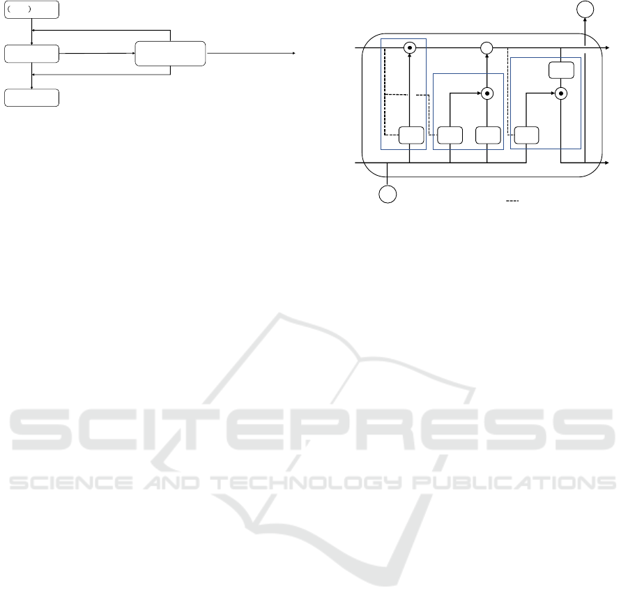
Figure 1: System overview utilizing the Sequential Evalu-

ation Network (SEN). Upon completion of training at the

N-th epoch, the internal parameters are fed into the pre-

trained SEN, which subsequently outputs one of three states

to autonomously control the training process: (i) Continue

Training: The training continues if high future accuracy is

anticipated with the current network size. (ii) Retrain the

Current Epoch: If the training results from the current epoch

adversely impact the internal state, retraining is initiated at

the same epoch. (iii) Retrain with Adjusted Network Size:

If the current network size is deemed to lack potential, the

network size is expanded, and retraining begins anew.

plethora of networks NAS evaluates, efﬁcient perfor-

mance estimation becomes vital. LCE has emerged

as an efﬁcient strategy for performance estimation

(Baker et al., 2018; Wistuba and Pedapati, 2019; Yan

et al., 2021). Another notable direction in NAS opti-

mizes for constraints typical of small computers, not

merely accuracy. For example, FBNet (Wu et al.,

2019) optimizes both accuracy and inference speed

on mobile devices by introducing Differentiable Neu-

ral Network Architecture Search (DNAS) which em-

ploys an Operator Latency LUT to balance accuracy

with inference speed.

As elaborated, assessing the model’s potential

early on proves beneﬁcial for NAS tasks, emphasiz-

ing not only accuracy but also lightweightness. In

this study, we aim to construct a Sequential Evalu-

ation Network (SEN) that incrementally assesses a

model’s potential. SEN strives for balanced learn-

ing in terms of accuracy and network size by eval-

uating the model’s potential during training and au-

tonomously controlling the training process. Our ap-

proach distinctively centers on the network’s internal

state rather than on validation accuracy, akin to LCE.

We posit that by honing in on the internal state, we

can gauge the latent potential of a model, unreﬂected

in the network output, enabling more efﬁcient train-

ing control. Moreover, computing validation accu-

racy every epoch using large datasets and metrics such

as Average Precision (AP) can be resource-intensive.

In contrast, SEN, bypassing validation accuracy, as-

sesses the model’s potential in a more lightweight

manner. Figure 1 illustrates the system overview us-

ing SEN. Training initiates with an extremely small

network size, expanding until SEN anticipates higher

accuracy in the future, thereby efﬁciently training a

model that balances accuracy and network size.

ℎ

𝑥

𝜌, 𝜎 ∶ activation function

: peephole connections

𝑐

!"#

ℎ

!"#

𝑓

𝑖

𝑜

𝑐

ℎ

forget gate

input gate

output gate

𝜎 𝜎 𝜌 𝜎

𝜌

Figure 2: Schematic of an LSTM block, illustrating data

ﬂow through input, forget, and output gates along with the

memory cell. Equations (1)–(6) describe the interactions

and updates within the block.

In this paper, as a foundamental study for con-

structing SEN, we explore a trafﬁc accident predic-

tion network employing onboard monocular camera

footage as our subject of investigation. One such

network is the Dynamic Spatial Attention - Recur-

rent Neural Network (DSA-RNN) (Chan et al., 2016).

DSA-RNN chieﬂy consists of an image feature ex-

traction component and a temporal data processing

component. Generally, CNNs used for image feature

extraction in such systems leverage pretrained mod-

els, with training commonly reserved for the temporal

data processing network. Consequently, In this study,

our aim is to optimize the accuracy and network size

of LSTM (Long Short-Term Memory) used for pro-

cessing time-series data. To achieve this, we closely

examine the internal states of the LSTM and aim to

evaluate the potential of the model during training on

a step-by-step basis.

2 RELATED WORK

2.1 LSTM

Recurrent Neural Networks (RNNs) are commonly

cited as foundamental architectures for processing

time series data. These networks possess a unique

structure characterized by self-recursive connections

across time. Speciﬁcally, the intermediate activa-

tion feature h

t−1

from a given timestep is integrated

with the input x

of the subsequent timestep. Al-

though RNNs are engineered to process time series

data, they suffer from the vanishing gradient prob-

lem (Pascanu et al., 2013), which hampers long-term

learning. LSTM addresses this issue by substituting

the hidden layer nodes with LSTM blocks, as illus-

VISAPP 2024 - 19th International Conference on Computer Vision Theory and Applications

318

trated in Figure 2.

LSTM is architected around a Constant Error

Carousel (CEC, also known as a memory cell), an in-

put gate, a forget gate, and an output gate. The mem-

ory cell in an LSTM retains information over multiple

time steps. The forget gate determines the fraction of

long-term memory from the preceding time step to

retain, while the input gate decides the amount of cur-

rent input or short-term memory to store in the mem-

ory cell, effectively updating its state. The output gate

then decides how much information should be emit-

ted based on the current internal state. The output at

time t is recurrently used as input for the LSTM block

at the subsequent timestep t + 1. As illustrated in Fig-

ure 2, the input at time t is represented by x

, and the

output is denoted by h

Assuming the quantity of LSTM blocks is N and

the number of inputs is M, the weight, serving as the

learning parameter, is described as:

• Input weights:

, W

∈ R

N×M

• Recurrent weights:

, R

∈ R

N×N

• Peephole connection weights:

, p

∈ R

• Bias: b

, b

∈ R

Moreover, the variables z

, f

, i

, o

, and c

cor-

respond to the input to the LSTM block, the forget

gate, the input gate, the output gate, and the memory

cell at time t, respectively. These are deﬁned by the

following equations:

= ρ(W

+ R

t−1

+ b

) (1)

= σ(W

+ R

t−1

+ p

⊙ c

t−1

+ b

) (2)

= σ(W

+ R

t−1

+ p

⊙ c

t−1

+ b

) (3)

= σ(W

+ R

t−1

+ p

⊙ c

+ b

) (4)

= z

⊙ i

+ c

t−1

⊙ f

(5)

= ρ(c

) ⊙ o

(6)

In these equations, ⊙ symbolizes the Hadamard

product. Typically, the sigmoid function (σ(x) =

1/(1 + e

−x

)) serves as the activation function for the

gates, while the hyperbolic tangent function is utilized

for both input and output activations.

Due to the incorporation of memory cells and di-

verse gates, LSTM can process extensive time se-

ries data more effectively than conventional RNNs.

Hence, in recent times, deep learning techniques for

time series data processing have found applications

in various sectors, such as video and motion picture

analysis, linguistic processing, and audio processing.

In the analysis of LSTM’s internal parameters (Gr-

eff et al., 2017), the impact on performance when cer-

tain parameters are omitted is discussed. Notably, the

performance degradation is substantial when remov-

ing the forget gate and the activation function of the

output. This indicates that within the LSTM, the for-

get gate and the output’s activation function play cru-

cial roles. A visualization study of the LSTM (Karpa-

thy et al., 2016) examined each LSTM cell’s opera-

tion. It has been mentioned that LSTM cells, existing

in multiple within the hidden layers, have variations

in their behaviors. In particular, when focusing on

the values of the forget gate, it has been reported that

there are cells that operate to retain memory over a

long period of time. However, some cells are not eas-

ily interpretable. Therefore, we assume that models

with a higher proportion of highly active cells amidst

a mixture of highly and less active cells in the hid-

den layer have potential for the future. We deﬁne the

activity level of LSTM cells using the value of the

forget gate, which has been reported to particularly

contribute to accuracy.

2.2 Trafﬁc Accident Prediction Using

DSA-RNN

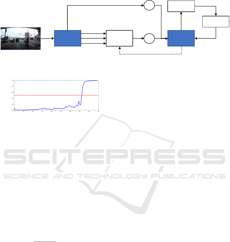
Figure 3 presents the model visualization of DSA-

RNN, which is designed to predict trafﬁc accidents

using an LSTM based on information acquired from

an onboard monocular camera. The input to the DSA-

RNN at time t is a frame image whose features x

are

generated by passing the frame through a CNN. Al-

though these frame features capture the overall char-

acteristics of the image, they might not effectively

capture the details of objects, such as four-wheeled

or two-wheeled vehicles, appearing only in parts of

the image.

In order to address this limitation, the Dynamic

Spatial Attention (DSA) mechanism is proposed to

extract object features x

focused on potentially haz-

ardous objects within the image. By providing the

LSTM with both the object features x

extracted by

the DSA and the frame features x

, the surrounding

environment is considered during trafﬁc accident pre-

diction.

The features of each potentially hazardous object

detected by Faster R-CNN (Ren et al., 2015) are rep-

resented as

, and the importance of each hazardous

object is given by α

. Here, J denotes the number

of potentially hazardous objects, with j indexing each

object from 1 to J. The object features x

obtained by

the DSA are computed as in Equation (7), where the

importance of each object α

is computed according

Evaluating Learning Potential with Internal States in Deep Neural Networks

319

!!𝒙

𝑿

𝒉

!"#

Figure 3: Architecture of the DSA-RNN model, integrating frame features, x

, and dynamically-attended object features, x

for trafﬁc accident prediction using the LSTM and onboard monocular camera inputs.

Time step

Probability of accident

Threshold

Figure 4: Temporal evolution of the DSA-RNN’s pre-

dicted accident probability (solid blue line) across sequen-

tial frames, triggering an accident prediction when exceed-

ing a predeﬁned threshold (red dashed line).

to Equation (8). In Equation (8), the term e

is calcu-

lated as shown in Equation (9). In this formulation, w

, U

, and b

are training parameters, and h

t−1

rep-

resents the activation feature of the LSTM from the

preceding time step.

As shown in Figure 4, the network computes the

probability of an accident at each time step. When

the accident probability, represented by the solid blue

line, surpasses the threshold indicated by the red

dashed line, a trafﬁc accident is predicted to occur in

that scene.

= DSA(X

,α

) =

∑

j=1

(7)

exp(e

)

∑

exp(e

)

(8)

= w

ρ(W

t−1

+ b

) (9)

3 PROPOSED METHOD

We assume that within the hidden layers where mul-

tiple LSTM cells exist, there is a mix of cells with

high and low activity levels, and the higher the pro-

portion of highly active cells, the more promising the

model is. Therefore, we focus on the values of the

LSTM’s forget gate to deﬁne the activity level of the

LSTM cells. Moreover, based on the aforementioned

assumption, we deﬁne an overall activity level met-

ric for the LSTM. This metric aggregates the activity

level information across all LSTM cells and serves as

an indicator of the model’s potential. A mathematical

formulation of the activity level metric, based on the

forget gate values, could provide a quantiﬁable mea-

sure of the model’s potential, enabling more objective

evaluations and comparisons.

3.1 Deﬁnition of Highly Active LSTM

Cells

The LSTM uses a forget gate to regulate the degree

of memory retention from the previous time step. At

time t, the forget gate f

is an N-dimensional vec-

tor, where N denotes the number of nodes in the hid-

den layer, represented as f

= ( f

.. . f

)

. As

indicated in Equation (5), if the value of the forget

gate f

(k ∈ 1,...,N) is 1, the memory is entirely re-

tained. Conversely, a value of 0 leads to complete

memory forgetting. With appropriate timing of its for-

getting mechanism, the LSTM can process consider-

ably longer sequences compared to RNN and effec-

tively handle changes in conditions. In accident pre-

diction scenarios, a rapid decrease in the forget gate

value might signify a transition from a safe to a haz-

ardous situation. This allows the LSTM to integrate

information in dangerous scenarios more effectively.

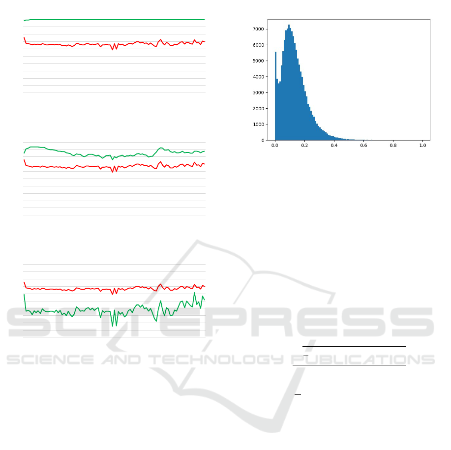
Considering the operation of the forget gate, we dis-

cuss three types, as represented in Figures 5a to 5c.

In these ﬁgures, the red solid line depicts the aver-

age transition of the forget gate value f

for all cells,

and the green solid line illustrates the transition of

the forget gate value f

for a speciﬁc cell. Figure

5a showcases a cell that maintains memory by persis-

tently transitioning at values near its maximum. Fig-

ure 5b represents a cell mirroring the average transi-

tion of the forget gate value. Figure 5c typiﬁes a cell

with signiﬁcant ﬂuctuations, differing from the mean

VISAPP 2024 - 19th International Conference on Computer Vision Theory and Applications

320

0.0

0.1

0.2

0.3

0.4

0.5

0.6

0.7

0.8

0.9

1.0

0 10 20 30 40 50 60 70 80 90

Forget gate activation

Time step

(a) Persistent Memory Retention

0.0

0.1

0.2

0.3

0.4

0.5

0.6

0.7

0.8

0.9

1.0

0 10 20 30 40 50 60 70 80 90

Forget gate activation

Time step

(b) Average Transition

0.0

0.1

0.2

0.3

0.4

0.5

0.6

0.7

0.8

0.9

1.0

0 10 20 30 40 50 60 70 80 90

Forget gate activation

Time step

Figure 5: Transitions of forget gate values of LSTM cells

demonstrating different behaviors: (a) Persistent mem-

ory retention, (b) Typical average transition, and (c) No-

table ﬂuctuations representing responsiveness to situational

changes. Red and green lines depict average and speciﬁc

cell forget gate values, respectively.

transition. LSTM cells with pronounced ﬂuctuations,

such as those shown in Figure 5c, indicate their re-

sponsiveness to sudden situational changes.

Here, based on the magnitude of local variations

in the values of the forget gate, we deﬁne the LSTM

Cell Activity Level (LCAL). The LCAL of the LSTM

cell k is deﬁned in Equation (10). In the equation,

(t) is the coefﬁcient of variation of the values of

the forget gate, as shown in Equation (11). The coef-

ﬁcient of variation is calculated for each moving av-

erage of window size w, as shown in Equation (12).

When evaluating the variability of the forget gate’s

values solely by the standard deviation, it is believed

that there would be little difference in the variability

across windows. Therefore, by using the mean value,

which is less than 1, to subtract from the standard de-

LCAL

The number of LSTM cells

Figure 6: Histogram of LCAL across all LSTM cells for

TrueP scenes. LCAL values are calculated for each of

the N · TP patterns arising from N hidden layers and TP

TrueP scenes, revealing the distribution of activity levels

within the network during accurate accident prediction. The

LSTM Activity Level (LAL) is subsequently derived from

these distributions, offering insight into the potential of the

model based on the prevalence of high-activity LSTM cells.

viation, a form of weighting is applied, making the

differences in variability more pronounced. Further-

more, by calculating the variation using moving aver-

ages, we derive the local variation amount of the val-

ues of the forget gate, and deﬁne its maximum value

as LCAL.

LCAL

= max

(t) (10)

(t) =

∑

t+w−1

i=t

( f

− MA

(t)))

MA(t)

(11)

(t) =

t+w−1

∑

i=t

(12)

3.2 Deﬁnition of the Overall Activity

Level of LSTM

We assume that the higher the proportion of LSTM

cells with a large LCAL when viewed across the en-

tire hidden layer, the more potential the model has.

Based on this assumption, we deﬁne the LSTM Activ-

ity Level (LAL). In the context of trafﬁc accident pre-

diction, we consider the scenes where the forget gate

value is most activated to be the scenes where acci-

dents are correctly predicted when they occur, and we

denote such scenes as TrueP. We calculate the LCAL

for all scenes that are TrueP. At this time, if we denote

the total number of TrueP scenes as TP, then there ex-

ist TP states of hidden layers. In other words, if we

denote the number of hidden layers as N, N · TP pat-

terns of LCAL are calculated. These LCALs are rep-

resented in a single histogram, as shown in Figure 6.

Evaluating Learning Potential with Internal States in Deep Neural Networks

321

As shown in Figure 5a, the LCAL value of the cell is

close to 0. Given this, we expect the LCAL histogram

to be concentrated around the value of 0. Therefore,

as shown in Equation (13), we deﬁne LAL as the pro-

portion of LSTM cells with an LCAL greater than a

threshold τ

LAL

. Here, the function I(·) acts as an indi-

cator function, returning 1 if the condition is met and

0 otherwise.

LAL =

N · TP

∑

k=1

∑

TrueP=1

I(LCAL

TrueP

≥ τ

LAL

)

(13)

4 EXPERIMENT

4.1 Experiment Details

In this section, we provide a detailed description

of the preliminary experiments aimed at construct-

ing SEN for trafﬁc accident prediction. For this ex-

periment, we utilized the Dashcam Accident Dataset

(DAD) (Chan et al., 2016) and trained it for 30

epochs. Herein, we denote the models with hidden

layer sizes set to 128, 512, 1024, and 2048 as M

128

512

, M

1024

, and M

2048

, respectively. As LSTM’s in-

ternal states change with each training iteration, we

trained the M

128

, M

512

, M

1024

, and M

2048

models ten

times each. Subsequently, we conducted preliminary

experiments on these trained models using the ana-

lytical methods described in Section 3. The experi-

ments were conducted using TensorFlow on a server

equipped with an NVIDIA RTX A6000 GPU.

4.1.1 Details of the Dashcam Accident Dataset

The DAD consists of dashcam footage capturing ve-

hicular and motorcycle accidents shot in Taiwan.

Each video clip is recorded at 20fps, spanning 100

frames, or a total duration of 5 seconds. For clips con-

taining accidents, the actual accident event is captured

between the 90th and 100th frames. As a result, the

90 frames leading up to the accident are used to pre-

dict its occurrence. For this experiment, the dataset

comprises a total of 620 videos with accidents (455

for training and 165 for validation) and 1,130 videos

without accidents (829 for training and 301 for vali-

dation).

4.1.2 Evaluation Metrics

For evaluating the activity level of LSTM cells, we

use the LCAL set with a window size w = 5. In the

DAD dataset, as the last 10 frames of the accident-

inclusive videos contain the actual accident, the in-

terval (90, 100] is excluded from evaluation. Addi-

tionally, due to the network output’s instability in the

initial frames, the interval [1, 10) is also excluded.

Therefore, the LCAL is calculated using the moving

average in the interval [10,90]. Moreover, as an in-

dicator of the model’s potential, we use LAL with a

threshold τ

LAL

= 0.05.

For assessing the accuracy of trafﬁc accident pre-

diction, we use Average Precision (AP). In scenes

containing an accident, the number of scenes cor-

rectly predicted to have an accident is termed True

Positive (TP), while the number of scenes mistakenly

predicted as non-accidental is labeled False Negative

(FN). Conversely, in non-accident scenes, scenes in-

correctly predicted to have an accident are designated

as False Positive (FP), and those accurately predicted

without an accident are labeled True Negative (TN).

Using these metrics, Recall and Precision are com-

puted for each accident threshold to derive the AP.

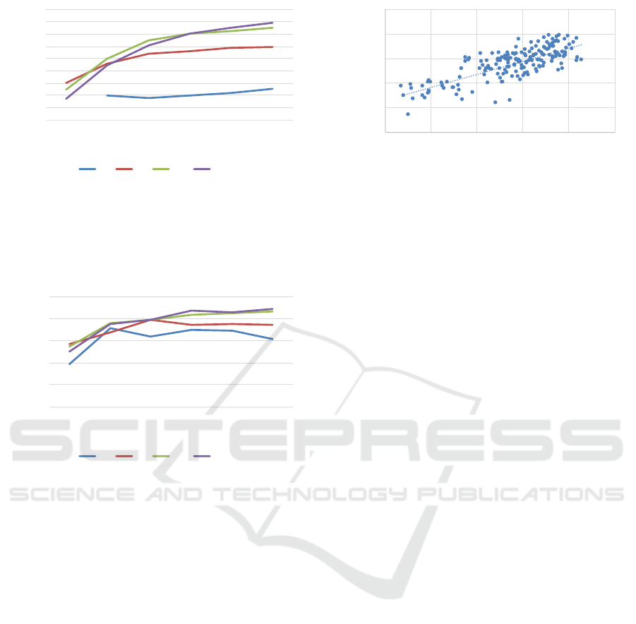
4.2 Results

4.2.1 Transition of LSTM Activity Levels

For the models M

128

, M

512

, M

1024

, and M

2048

trained

10 times each, we calculated LAL and AP at epochs

5, 10, 15, 20, 25, and 30. We then recorded the tran-

sition of the average LAL and AP over the epochs

for each model. Notably, for some epochs of M

128

and M

512

(primarily at epoch 5), there were no scenes

with TrueP, making it impossible to compute LAL.

Hence, we plotted the average of the available LAL

data. The transitions of LAL and AP are depicted in

Figures 7 and 8, respectively.

When focusing on the AP of M

128

, it is evident

that the training was not very effective, registering the

lowest value at epoch 30. On the other hand, by ex-

amining the LAL, its value was comparable to other

models during the early training phases. However, as

training progressed, there was minimal growth, set-

ting at a lowest value by epoch 30. The ﬂuctuations in

AP suggest that the number of LSTM cells may be in-

sufﬁcient, indicating that the hidden layer size might

be inadequate for retaining essential information for

trafﬁc accident predictions. Especially when consid-

ering the LAL outcomes, we deduce that the model

might not achieve higher accuracy moving forward,

as the number of ”active” cells, anticipated to increase

with more epochs, remains stagnant. A similar trend

is visible with the results for M

512

. In terms of AP,

compared to the outcomes of M

1024

and M

2048

, it is

clear that the training was less effective. Likewise,

concerning LAL, its growth rate is slower, settling at

a lower value by epoch 30. From the above, it can

VISAPP 2024 - 19th International Conference on Computer Vision Theory and Applications

322

0.1

0.2

0.3

0.4

0.5

0.6

0.7

0.8

0.9

5 10 15 20 25 30

LAL

epoch

128 512 1024 2048

Figure 7: Epoch-wise Transition of LSTM Activity Levels

(LAL) for Models M

128

, M

512

, M

1024

, and M

2048

. The plot

illustrates the progression and potential stability of LAL

across different model complexities and provides insights

into the effective hidden layer size during the training for

accident prediction.

0.5

0.55

0.6

0.65

0.7

0.75

5 10 15 20 25 30

epoch

128 512 1024 2048

Figure 8: Epoch-wise Transition of Average Precision (AP)

for Models M

128

, M

512

, M

1024

, and M

2048

. The graph

demonstrates the predictive performance of each model

over the epochs and aids in understanding the model’s efﬁ-

ciency in predicting trafﬁc accidents throughout the training

process.

be inferred that for models with a hidden layer size

of 128 and 512, the potential is not promising, thus in

SEN, we believe that increasing the size of the hidden

layer and retraining is effective.

Additionally, analyzing the results for M

1024

and

2048

, both AP and LAL appear to be nearly iden-

tical. This observation leads us to conclude that aug-

menting the number of LSTM cells beyond this might

only result in convergence to similar values, aiding in

determining the optimal LSTM cells count. In other

words, we consider it effective to continue training

with the current parameters in SEN.

In summation, the observed relationship between

the increase in LAL and AP values during training in-

dicates that by monitoring changes in LAL values, we

can discern whether to prolong training or if the cur-

rent hidden layer size is promising for future accuracy

enhancements.

0.55

0.6

0.65

0.7

0.75

0.8

0 0.2 0.4 0.6 0.8 1

LAL

Figure 9: Correlation Analysis between LSTM Activity

Levels (LAL) and Average Precision (AP). The scatter plot

represents models M

512

, M

1024

, and M

2048

, each at epochs

5, 10, 15, 20, 25, and 30, suggesting a signiﬁcant positive

correlation (0.767) that implies the potentiality of LAL as a

predictive indicator of model accuracy in future epochs.

4.2.2 Correlation Between LSTM Activity

Levels and Accuracy

We investigated the correlation between LAL and AP

for the models M

512

, M

1024

, and M

2048

. We excluded

128

due to its notably low LAL. Data was plotted

for LAL and AP at epochs 5, 10, 15, 20, 25, and 30,

for each model trained 10 times. The results are de-

picted in Figure 9. A correlation coefﬁcient of 0.767

indicates a signiﬁcant positive relationship. From the

foregoing, we believe that by extrapolating the LAL

in the early stages of training, it is possible to predict

future accuracy.

However, there currently remains a challenge re-

garding the computational cost of LAL. The distinct

aspect of the intended SEN from existing methods

is that, unlike the time-consuming validation accu-

racy calculated per epoch with a large amount of data

using AP or other evaluation methods, it employs

a lightweight evaluation metric using internal states.

Therefore, it’s necessary to keep the computation cost

of LAL low. The high computation cost stems from

the fact that the validation data used for calculating

AP is also employed to extract the scenes for TrueP,

which is used in the calculation of LAL. It is sufﬁcient

to use only the data containing accidents to extract the

scenes for TrueP. Additionally, since the LCAL his-

togram is created by integrating histograms of sim-

ilar trends obtained for each scene being TrueP, we

believe that a lesser total number of TrueP is accept-

able. Hence, there is a need to experiment whether

a positive correlation between LAL and accuracy can

be obtained using validation data constituted only of

a small number of accident-inclusive videos for the

computation of LAL.

Evaluating Learning Potential with Internal States in Deep Neural Networks

323

5 CONCLUSION

This study aims at efﬁcient learning of models that

balance accuracy and network scale as its goal. We

are also targeting the construction of SEN, which

evaluates the potential of a model utilizing the inter-

nal states of the network. In this paper, we focused on

the LSTM in the trafﬁc accident prediction network

and deﬁned the activity level of LSTM cells based on

the variation in the values of the forget gate. More-

over, we assumed that a model has more potential if

the proportion of high-activity LSTM cells is higher,

and hence deﬁned LAL. By checking the transition of

LAL and AP, we demonstrated that the value of LAL

is effective for controlling SEN. Additionally, since a

positive correlation between LAL and AP was con-

ﬁrmed, we believed that it’s possible to predict future

accuracy by extrapolating LAL in the early stages of

training.

In our future research, ﬁrstly, we plan to create a

small validation data set for the calculation of LAL

and experiment on the effectiveness of LAL calcu-

lated at a low cost. Then, we will proceed to discuss

the speciﬁc methods of extrapolating LAL.

REFERENCES

Baker, B., Gupta, O., Raskar, R., and Naik, N. (2018).

Accelerating neural architecture search using perfor-

mance prediction. In International Conference on

Learning Representations.

Chan, F. H., Chen, Y. T., Xiang, Y., and Sun, M. (2016).

Anticipating accidents in dashcam videos. In Asian

Conference on Computer Vision, pages 136–153.

Chen, Y., Yang, T., Zhang, X., Meng, G., Xiao, X., and

Sun, J. (2019). Detnas: Backbone search for object

detection. In International Conference on Neural In-

formation Processing Systems.

Domhan, T., Springenberg, J. T., and Hutter, F. (2015).

Speeding up automatic hyperparameter optimization

of deep neural networks by extrapolation of learning

curves. In International Joint Conference on Artiﬁcial

Intelligence, pages 3460–3468.

Greff, K., Srivastava, R. K., Koutnık, J., Steunebrink, B. R.,

and Schmidhuber, J. (2017). Lstm: A search space

odyssey. IEEE Transactions on Neural Networks and

Learning Systems, pages 2222–2232.

Hutter, F., Kotthoff, L., and Vanschoren, J., editors (2019).

Automatic Machine Learning: Methods, Systems,

Challenges. Springer. In press, available at http:

//automl.org/book.

Karpathy, A., Johnson, J., and Fei-Fei, L. (2016). Visualiz-

ing and understanding recurrent networks. In Interna-

tional Conference on Learning Representations.

Klein, A., Falkner, S., Springenberg, J. T., and Hutter, F.

(2017). Learning curve prediction with bayesian neu-

ral networks. In International Conference on Learn-

ing Representations.

Liu, C., Chen, L.-C., Schroff, F., Adam, H., Hua, W., Yuille,

A., and Fei-Fei, L. (2019). Auto-deeplab: Hierarchi-

cal neural architecture search for semantic image seg-

mentation. In IEEE / CVF Computer Vision and Pat-

tern Recognition Conference.

Pascanu, R., Mikolov, T., and Bengio, Y. (2013). On the

difﬁculty of training recurrent neural networks. In In-

ternational Conference on Machine Learning, pages

1310–1318.

Real, E., Aggarwal, A., Huang, Y., and Le, Q. V. (2019).

Regularized evolution for image classiﬁer architecture

search. In AAAI Conference on Artiﬁcial Intelligence.

Ren, S., He, K., Girshick, R., and Sun, J. (2015). Faster

r-cnn: Towards real-time object detection with region

proposal networks. In IEEE / CVF Computer Vision

and Pattern Recognition Conference.

Swersky, K., Snoek, J., and Adams, R. P. (2014). Freeze-

thaw bayesian optimization. arXiv:1406.3896.

Wang, N., Gao, Y., Chen, H., Wang, P., Tian, Z., Shen, C.,

and Zhang, Y. (2020). Nas-fcos: Fast neural architec-

ture search for object detection. In IEEE / CVF Com-

puter Vision and Pattern Recognition Conference.

Wistuba, M. and Pedapati, T. (2019). Inductive transfer for

neural architecture optimization. arXiv:1903.03536.

Wu, B., Dai, X., Zhang, P., Wang, Y., Sun, F., Wu, Y., Tian,

Y., Vajda, P., Jia, Y., and Keutzer, K. (2019). Fbnet:

Hardware-aware efﬁcient convnet design via differen-

tiable neural architecture search. In IEEE / CVF Com-

puter Vision and Pattern Recognition Conference.

Yan, S., White, C., Savani, Y., and Hutter, F. (2021).

Nas-bench-x11 and the power of learning curves.

arXiv:2111.03602.

Zhang, Y., Qiu, Z., Liu, J., Yao, T., Liu, D., and Mei, T.

(2019). Customizable architecture search for semantic

segmentation. In IEEE / CVF Computer Vision and

Pattern Recognition Conference.

Zoph, B., Vasudevan, V., Shlens, J., and Le, Q. V. (2018).

Learning transferable architectures for scalable image

recognition. In IEEE / CVF Computer Vision and Pat-

tern Recognition Conference.

VISAPP 2024 - 19th International Conference on Computer Vision Theory and Applications

324