Interactively Teaching an Inverse Reinforcement Learner with Limited

Feedback

Rustam Zayanov

, Francisco S. Melo

and Manuel Lopes

INESC-ID & Instituto Superior T

ecnico, Universidade de Lisboa, Portugal

Keywords:

Sequential Decision Processes, Inverse Reinforcement Learning, Machine Teaching, Interactive Teaching and

Learning.

Abstract:

We study the problem of teaching via demonstrations in sequential decision-making tasks. In particular, we

focus on the situation when the teacher has no access to the learner’s model and policy, and the feedback from

the learner is limited to trajectories that start from states selected by the teacher. The necessity to select the

starting states and infer the learner’s policy creates an opportunity for using the methods of inverse reinforce-

ment learning and active learning by the teacher. In this work, we formalize the teaching process with limited

feedback and propose an algorithm that solves this teaching problem. The algorithm uses a modiﬁed version

of the active value-at-risk method to select the starting states, a modiﬁed maximum causal entropy algorithm

to infer the policy, and the difﬁculty score ratio method to choose the teaching demonstrations. We test the

algorithm in a synthetic car driving environment and conclude that the proposed algorithm is an effective so-

lution when the learner’s feedback is limited.

1 INTRODUCTION

Machine Teaching (MT) is a computer science ﬁeld

that formally studies a learning process from a

teacher’s point of view. The teacher’s goal is to teach

a target concept to a learner by demonstrating an op-

timal (often the shortest) sequence of examples. MT

has the potential to be applied to a wide range of prac-

tical problems (Zhu, 2015; Zhu et al., 2018), such

as: developing better Intelligent Tutoring Systems for

automated teaching for humans, developing smarter

learning algorithms for robots, determining the teach-

ability of various concept classes, testing the validity

of human cognitive models, and cybersecurity.

One promising application domain of MT is the

automated teaching of sequential decision skills to

human learners, such as piloting an airplane or per-

forming a surgical operation. In this domain, MT can

be combined with the theory of Inverse Reinforce-

ment Learning (IRL) (Ng et al., 2000; Abbeel and Ng,

2004), also known as Inverse Optimal Control. IRL

formally studies algorithms for inferring an agent’s

goal based on its observed behavior in a sequential de-

cision setting. Assuming that a learner will use a spe-

https://orcid.org/0009-0006-5301-6382

https://orcid.org/0000-0001-5705-7372

https://orcid.org/0000-0002-6238-8974

ciﬁc IRL algorithm to process the teacher’s demon-

strations, the teacher could pick an optimal demon-

stration sequence for that algorithm.

Most MT algorithms assume that the teacher

knows the learner’s model, that is, the learner’s al-

gorithm of processing demonstrations and converting

them into knowledge about the target concept. In the

case of human cognition, formalizing and verifying

such learner models is still an open research ques-

tion. The scarcity of such models poses a challenge to

the application of MT to automated human teaching.

One way of alleviating the necessity of a fully deﬁned

learner model is to develop MT algorithms that make

fewer assumptions about the learner. In the sequential

decision-making domain, (Kamalaruban et al., 2019)

and (Yengera et al., 2021) have proposed teaching al-

gorithms that admit some level of uncertainty about

the learner model. In particular, their teaching algo-

rithms assume that the learner’s behavior (policy) is

maximizing some reward function, but it is unknown

how the learner updates that reward function given the

teacher’s demonstrations. To cope with this uncer-

tainty, the teacher is allowed to observe the learner’s

behavior during the teaching process and infer the

learner’s policy from the observed trajectories, thus

making the process iterative and interactive.

Both works assume that the teacher can period-

Zayanov, R., Melo, F. and Lopes, M.

Interactively Teaching an Inverse Reinforcement Learner with Limited Feedback.

DOI: 10.5220/0012296800003636

Paper published under CC license (CC BY-NC-ND 4.0)

In Proceedings of the 16th International Conference on Agents and Artiﬁcial Intelligence (ICAART 2024) - Volume 1, pages 15-24

ISBN: 978-989-758-680-4; ISSN: 2184-433X

ically observe many learner’s trajectories from every

initial state and thus estimate the learner’s policy with

high precision. Unfortunately, the need to produce

many trajectories from every initial state may be un-

feasible in real-life scenarios. In our present work, we

address a more realistic scenario in which the feed-

back from the learner is limited to just one trajec-

tory per each iteration of the teaching process. The

limit on the learner’s feedback poses a challenge for

the teacher in reliably estimating the learner’s policy,

which, in turn, may diminish the usefulness of the

teacher’s demonstrations. Thus, our research ques-

tion is: What are the effective ways of teaching an

inverse reinforcement learner when the learner’s

policy and update algorithm are unknown, and the

learner’s feedback is limited?

The teacher’s ability to precisely estimate the

learner’s policy greatly depends on the informative-

ness of the received trajectories. We consider two

scenarios: an unfavorable scenario when the teacher

has no inﬂuence on what trajectories it will receive,

and a more favorable scenario when the teacher can

choose the states from which the learner will generate

trajectories. The necessity to select the starting states

creates an opportunity for the teacher to use methods

of Active Learning (AL) (Settles, 2009). In the con-

text of sequential decision-making, AL considers sit-

uations when a learner has to infer an expert’s reward

and can interactively choose the states from which

the expert’s demonstrations should start (Lopes et al.,

2009).

The contribution of our work is two-fold. Firstly,

we propose a new framework that formalizes interac-

tive teaching when the learner’s feedback is limited.

Secondly, we propose an algorithm for teaching with

limited feedback. The algorithm performs three steps

per every teaching iteration: selection of a query state

(AL problem), inference of the current learner’s pol-

icy (IRL problem), and selection of a teaching demon-

stration (MT problem). The algorithm uses a modi-

ﬁed version of the Active-VaR (Brown et al., 2018)

method for choosing query states, a modiﬁed ver-

sion of the Maximum Causal Entropy (MCE) (Ziebart

et al., 2013) method for inferring the learner’s policy,

and the difﬁculty score ratio (DSR) (Yengera et al.,

2021) method for selecting the teaching demonstra-

tion We test the algorithm in a synthetic car driving

environment and conclude that it is a viable solution

when the learner’s feedback is limited

The implementation of the algorithms is available at

https://github.com/rzayanov/irl-teaching-limited-feedback

2 RELATED WORK

(Liu et al., 2017) explore the problem of MT with un-

limited feedback in the domain of supervised learning

when the teacher and the learner represent the target

concept as a linear model. They consider a teacher

that does not know the feature representation and the

parameter of the learner. For this scenario, they in-

troduce an interaction protocol with unlimited learner

feedback, where the teacher can query the learner at

every step by sending all possible examples and re-

ceiving all learner’s output labels. (Liu et al., 2018)

continue this work and explore teaching with lim-

ited feedback in the same supervised learning setting.

Similarly to our work, the teacher can not request all

learner’s labels at every step but instead has to choose

which examples to query using an AL method.

(Melo et al., 2018) explore how interaction can

help when the teacher has wrong assumptions about

the learner. The authors focus on the problem of

teaching the learners that aim to estimate the mean

of a Gaussian distribution given scalar examples.

When the teacher knows the correct learner model,

the teaching goal is achieved after showing one ex-

ample. When it has wrong assumptions, and no in-

teraction is allowed, the learner approaches the cor-

rect mean only asymptotically. When interaction is

allowed, the teacher can query the learner at any time,

and the learner responds with the value of its current

estimate perturbed by noise. They show that this kind

of interaction signiﬁcantly boosts teaching progress.

(Cakmak and Lopes, 2012) and (Brown and

Niekum, 2019) propose non-interactive MT algo-

rithms for sequential decision-making tasks. Both

algorithms produce a minimal set of demonstrations

that is sufﬁcient to reliably infer the reward func-

tion. Both algorithms are agnostic of the learner

model and don’t specify the order of demonstrations,

which might be crucial for teaching performance if

the learner is not capable of processing the whole set

at once. The algorithm of (Cakmak and Lopes, 2012)

is based on the assumptions that the reward is a lin-

ear combination of state features and that the teacher

will provide enough demonstrations for the learner

to estimate the teacher’s expected feature counts re-

liably. With these assumptions, each demonstrated

state-action pair induces a half-space constraint on

the reward weight vector. Assuming that the learner

weights are bounded, it is possible to estimate the

volume of the subspace deﬁned by any set of such

constraints. A smaller volume means less uncertainty

regarding the true weight vector. Thus, demonstra-

tions that minimize the subspace volume are pre-

ferred. The authors propose a non-interactive algo-

ICAART 2024 - 16th International Conference on Agents and Artiﬁcial Intelligence

rithm for choosing the demonstration set: at every

step, the teacher will pick a demonstration that min-

imizes the resulting subspace volume. (Brown and

Niekum, 2019) propose an improved non-interactive

MT algorithm called Set Cover Optimal Teaching

(SCOT). They ﬁrst deﬁne a policy’s behavioral equiv-

alence class (BEC) as a set of reward weights under

which that policy is optimal. A BEC of a demon-

stration given a policy is the intersection of half-

spaces formed by all state-action pairs present in

such demonstration. The authors propose ﬁnding the

smallest set of demonstrations whose BEC is equal

to the BEC of the optimal policy. Finding such a

set is a set-cover problem. The proposed algorithm

is based on generating m demonstrations from each

starting state and using a greedy method of picking

candidates.

(Kamalaruban et al., 2019) and (Yengera et al.,

2021) propose interactive MT algorithms for sequen-

tial decision-making tasks when the learner can pro-

cess only one demonstration at a time, but the feed-

back from the learner is unlimited or has a high limit.

(Kamalaruban et al., 2019) ﬁrst consider an omni-

scient teacher whose goal is to steer the learner toward

the optimal weight parameter and ﬁnd an effective

teaching algorithm. Next, they consider a less infor-

mative teacher that can not observe the learner’s pol-

icy and has no information about the learner’s feature

representations and the update algorithm. Instead of

directly observing the current learner’s policy π

, the

teacher can periodically request the learner to gener-

ate k trajectories from every initial state, thus estimat-

ing π

. The limitation of this approach is that the ne-

cessity to produce trajectories from every initial state

may be hard to implement in practice when k is high

or the number of initial states is high. (Yengera et al.,

2021) further explore the problem of teaching with

unlimited feedback and propose the difﬁculty score

ratio (DSR) algorithm.

They introduce the notion of a difﬁculty score of a

trajectory given a policy, which is proportional to its

conditional likelihood given that policy, and propose a

teaching algorithm that selects a trajectory that maxi-

mizes the ratio of difﬁculty scores of the learner’s pol-

icy and the target policy.

To the best of our knowledge, the problem of

teaching with limited feedback in the domain of se-

quential decision-making tasks has not yet been ad-

dressed in the literature.

3 PROBLEM FORMALISM

The underlying task to be solved by an agent is

formally represented as a Markov Decision Process

(MDP) denoted as M = (S , A, T, P

, γ, R

⋆

), where S

is the set of states, A is the set of actions, T(S

′

| s, a)

is the state transition probability upon taking action a

in state s, P

(S) is the initial state distribution, γ is the

discount factor, and R

⋆

: S → R is the reward function

to be learned.

A stationary policy is a mapping π that maps each

state s ∈ S into a probability distribution π(· | s) over

A. A policy can be executed in M, which will pro-

duce a sequence of state-action pairs called trajectory.

For any trajectory ξ = {s

, a

, . . . , s

, a

}, we will de-

note its i-th state and action as s

and a

, respectively.

Given a policy π, the state-value function V

(s), the

expected policy value V

, and the Q-value function

(s, a) are deﬁned as follows respectively:

(s) = E

∞

∑

t=0

R(S

) | π, T, S

= s

(1)

= E

S∼P

(S)] (2)

(s, a) = R(s) + γE

S∼T(·|s,a)

(S)] (3)

A policy π

⋆

is considered optimal if it has the highest

state-values for every state. For any MDP, at least

one optimal policy exists, which can be obtained via

the policy iteration method (Sutton and Barto, 2018).

4 FRAMEWORK FOR TEACHING

WITH LIMITED FEEDBACK

In this section, we present our contributions: the

framework for teaching with limited feedback and an

algorithm for solving the problem of teaching with

limited feedback.

We consider two entities that can execute policies

on M: a teacher with complete access to M and a

learner that can access all elements of M except the

reward function, which we denote as M \ R

⋆

. The

teacher and the learner can interact with each other it-

eratively, with every iteration consisting of ﬁve steps

described in Algorithm 1. In the ﬁrst step, the teacher

chooses a query state s

and asks the learner to gen-

erate a trajectory starting from s

. We assume that the

query states can only be selected from the set of initial

states, i.e., s

∈ S

= {s : P

(s) > 0}. In the second

step, the learner generates a trajectory ξ

by execut-

ing its policy starting from s

and sends it back to the

teacher. In the third step, the teacher uses the learner’s

trajectory to update its estimate of the learner’s cur-

rent reward

and policy

. In the fourth step, the

Interactively Teaching an Inverse Reinforcement Learner with Limited Feedback

teacher demonstrates the optimal behavior by gener-

ating a trajectory ξ

, which we call a demonstration,

and sending it to the learner. In the last step, the

learner learns from the demonstration to update its re-

ward R

and policy π

. The teaching process is termi-

nated when the teaching goal is achieved, in the sense

deﬁned below.

Algorithm 1: Framework for teaching with limited

feedback.

1: for i = 1, . . . , ∞ do

2: Teacher sends a query state s

and requests a

trajectory starting from it

3: Learner generates and sends a trajectory ξ

4: Teacher updates its estimate of the learner’s

reward

and policy

5: Teacher generates and sends a demonstration

6: Learner updates its reward R

and policy π

7: Stop if the teaching goal is achieved

8: end for

We consider the problem described above from

the perspective of a teacher that has limited knowl-

edge about the learner. We consider the following set

of assumptions:

• Access to State Features: Both the teacher and

the learner can observe the same d numerical fea-

tures associated with every state, formalized as a

mapping φ : S → R

. The (discounted) feature

counts are deﬁned for a trajectory ξ or for a policy

π and a state s as follows:

µ(ξ) =

∑

φ(s

) (4)

µ(π, s) = E



∑

φ(S

) | π, S

= s



(5)

• Rationality: At every iteration, the learner main-

tains some reward mapping R

and derives a sta-

tionary policy π

that is appropriate for R

, which

it uses to generate trajectories. The exact method

of deriving π

from R

is unknown to the teacher.

• Reward as a Function of Features: As it is com-

mon in the IRL literature, the learner represents

the reward as a linear function of state features:

(s) = ⟨θ

, φ(s)⟩, where the vector θ

is called the

feature weights. Furthermore, we assume that the

true reward R

⋆

can be expressed as a function of

these features, i.e., ∃θ

⋆

s.t. ∀s, R

⋆

(s) = ⟨θ

⋆

, φ(s)⟩.

• Learning from Demonstrations: Upon receiv-

ing a demonstration ξ

, the learner uses it to up-

date its parameter θ

i+1

and thus its reward R

i+1

Active

Learning

Inverse

Reinforcement

Learning

Demonstration ξ

Machine

Teaching

Query state s

Trajectory ξ

Learner's policy

estimate π̂

Teacher Learner

Policy

Learning

algorithm

Data from

iterations

Figure 1: The teaching algorithm can be divided into three

modules, each solving AL, IRL, or MT problem at every

iteration. This diagram shows the inputs and outputs of the

modules.

The exact method of updating θ

i+1

from ξ

is un-

known to the teacher.

There are different ways of evaluating the

teacher’s performance. In general, some notion of nu-

merical loss L

is deﬁned for every step (also called

the teaching risk), and the teacher’s goal is related to

the progression of that loss. Similarly to the previous

works, we will use a common deﬁnition of the loss as

the expected value difference (EVD): L

= V

⋆

−V

(Abbeel and Ng, 2004; Ziebart, 2010), when evalu-

ated against the real reward R

⋆

, and deﬁne the teach-

ing goal as achieving a certain loss threshold ε in the

lowest number of iterations.

Since the teacher has no access to π

, it has to

infer it from the trajectories received during teach-

ing, which corresponds to the problem of Inverse Re-

inforcement Learning. To infer π

effectively, the

teacher has to pick the query states with the highest

potential of yielding an informative learner trajectory,

which corresponds to the problem of Active Learn-

ing. Finally, to achieve the ultimate goal of improving

the learner’s policy value, the teacher must select the

most informative demonstrations to send, which cor-

responds to the problem of Machine Teaching. Since

a teaching algorithm has to solve these three problems

sequentially, it can be divided into three “modules”,

each module solving one problem. Figure 1 shows

the inputs and outputs of these modules.

We propose a concrete implementation of such

a teaching algorithm, which we call Teaching with

Limited Feedback (TLimF). It is formally described

in Algorithm 2. In the AL module, it uses the

Interactive-Value-at-Risk (VaR) algorithm, which is

a version of the Active-VaR algorithm (Brown and

Niekum, 2019) that we adapted to teaching with lim-

ited feedback. In the IRL module, TLimF uses the

Interactive-MCE algorithm, which is our adapted ver-

sion of the MCE-IRL algorithm (Ziebart et al., 2013).

Finally, in the MT module, it uses the DSR algorithm

ICAART 2024 - 16th International Conference on Agents and Artiﬁcial Intelligence

(Yengera et al., 2021). We describe all these three al-

gorithms below.

Algorithm 2: Teaching with Limited Feedback

(TLimF).

1: for i = 1, . . . , ∞ do

3: s

= Interactive-VaR(ξ

, . . . , ξ

i−1

) ▷ AL

step

4: Send s

to the learner, receive ξ

= Interactive-MCE(ξ

i−1

) ▷ IRL step

8: ξ

= DSR(

) ▷ MT step

9: Send ξ

to the learner

10:

11: Stop if V

⋆

− V

< ε

12: end for

4.1 Interactive-MCE

Our algorithm for the IRL module, Interactive-MCE,

is based on the MCE-IRL algorithm proposed by

(Ziebart et al., 2013).

The original algorithm searches for a solution in

the class MCE policies,

(a | s) = exp[βQ

soft

(s, a) − βV

soft

(s)], (6)

soft

(s, a) = ⟨θ, φ(s)⟩+γE

S∼T(·|s,a)

soft

(S)], (7)

soft

(s) =

log

∑

′

∈A

exp[βQ

soft

(s, a

′

)], (8)

where β is the entropy factor. For any θ, the

corresponding MCE policy can be found with the

soft-value iteration method (Ziebart, 2010). The

MCE-IRL algorithm looks for a parameter θ and a

policy π

that has the highest likelihood of producing

the observed set of trajectories Ξ, which is a convex

problem when the reward is linear. It can be solved

with the gradient ascent method, with the gradient

equal to

∇L(θ) =

|Ξ|

∑

(µ(ξ) − µ(π

, s

)). (9)

The original MCE-IRL algorithm assumes that all

the available trajectories were generated by a constant

policy that is based on a constant reward function.

However, in our situation, the trajectories received

from the learner are generated by different policies

based on different rewards since the learner is as-

sumed to update its reward function after receiving

every teacher demonstration. Thus, using all trajec-

tories simultaneously with the MCE-IRL algorithm

might infer a reward that is very different from the

actual learner’s reward.

We propose a sequential version of this algorithm.

At every interaction step i, this algorithm starts with

the previously inferred weights

i−1

and applies the

MCE gradient ascent with only the new trajectory ξ

as the evidence. Unlike a similar algorithm used by

the MCE learner in (Kamalaruban et al., 2019), which

performs only one MCE iteration per each new tra-

jectory, our variant performs the gradient ascent for

many iterations to better utilize the knowledge con-

tained in the trajectories. If the learner’s trajectories

are short, this method might overﬁt to the actions ob-

served in the latest trajectory. To avoid that, the older

trajectories could be included in the gradient update,

possibly with lower weight, or the feedback might

have to be increased to a higher number of trajectories

per iteration. Interactive-MCE is formally described

in Algorithm 3.

Algorithm 3: Interactive-MCE.

Require: trajectory ξ

, previous or initial estimate

i−1

1: s

= First-State(ξ

)

i−1

= Soft-Value-Iter(

)

4: for n = 1, . . . , N do

+ η

(µ

− µ

)

= Soft-Value-Iter(

)

7: end for

8: return

4.2 Interactive-VaR

Our algorithm for the AL module, Interactive-VaR,

is based on the Active-VaR algorithm proposed by

(Brown and Niekum, 2019).

The original algorithm assumes that the MDP is

deterministic, the reward weights lie on an L1-norm

unit sphere, and the expert is following a constant

parametrized softmax policy,

(a | s) =

exp[cQ

(s, a)]

∑

′

∈A

exp[cQ

(s, a

′

)]

, (10)

where c is a known conﬁdence factor and Q

are the

Q-values of an optimal policy for θ. For any reward

weights θ on the L1-norm unit sphere, the probability

of observing the given set of trajectories Ξ is

P(Ξ | θ) =

exp

∑

ξ∈Ξ

∑

, a

)

, (11)

Interactively Teaching an Inverse Reinforcement Learner with Limited Feedback

where Z is a normalizing constant. If the apriori dis-

tribution of θ is unknown, the probability of the given

weights θ generating the observed trajectories is

P(θ | Ξ) =

′

P(Ξ | θ). (12)

For any policy π, weights θ and starting state s, the

expected value difference (EVD) of π is deﬁned as

EVD(θ | π, s) = V

(s) − V

(s). (13)

The Active-VaR method proposes to choose the next

query state s

by ﬁnding the state that has the max-

imum VaR of EVD of the previously inferred policy

i−1

= argmax

s∈S

VaR[EVD(θ |

i−1

, s)] (14)

The original Active-VaR algorithm is not well-

suited for the problem in question because the obser-

vations were generated by different learner policies,

each corresponding to a different reward. One way of

addressing this problem is to give less weight to the

older observations when computing the likelihood of

any θ:

P(θ | ξ

, . . . , ξ

) ≈

∏

i=1

P(ξ

| θ)

(15)

= 1 (16)

lim

i→−∞

= 0 (17)

In particular, it is possible to consider only the last n

observations,

P(θ | ξ

, . . . , ξ

) ≈

∏

i=(k−n)

P(ξ

| θ) (18)

or to have the weight decay exponentially,

P(θ | ξ

, . . . , ξ

) ≈

∏

i=1

P(ξ

| θ)

k−i

, λ < 1. (19)

An additional advantage of the exponential decay is

computational speed because after receiving a new

trajectory, it is possible to compute the updated likeli-

hoods by reusing the likelihoods computed in the pre-

vious iteration:

∏

i=1

P(ξ

| θ)

k−i

= P

k−1

P(ξ

| θ). (20)

To avoid using several policy classes within the

compound teaching algorithm, we assume that the

learner follows an MCE policy instead of a softmax

policy. Given that, ﬁrstly, we use the soft Q-values of

the MCE policy to calculate the demonstration prob-

abilities:

P(ξ|θ) =

exp



∑

soft

, a

)



(21)

Secondly, for calculating VaR, we use the differ-

ence of the expected soft values: Soft-EVD(θ|π, s) =

soft,π

(s) − V

soft,π

(s). Finally, we replace the as-

sumption about the known softmax conﬁdence factor

c with a similar assumption about the known MCE

entropy factor β.

Interactive-MCE is formally described in Algo-

rithm 4.

Algorithm 4: Interactive Value-at-Risk (Interactive-

VaR).

Require: previous trajectories ξ

, . . . , ξ

, previous or

initial estimate

i−1

1: if i = 1 then

2: Pick a random initial state s

∈ S

3: else

4: Sample reward weights Θ

5: s

= argmax

s∈S

VaR[Soft-EVD(Θ |

i−1

, s)]

6: end if

7: return s

4.3 Difﬁculty Score Ratio

For deterministic MDPs, the difﬁculty score of a

demonstration ξ w.r.t. a policy π is deﬁned as

Ψ(ξ) =

∏

π(a

| s

)

(22)

The DSR algorithm selects the next teacher’s demon-

stration ξ

by iterating over a pool of candidate trajec-

tories Ξ and ﬁnding the trajectory with the maximum

difﬁculty score ratio. DSR is formally described in

Algorithm 5.

Algorithm 5: Difﬁculty Score Ratio (DSR).

Require: Policy estimate

1: for ξ in candidate pool Ξ do

(ξ) =

∏

| s

)

−1

3: Ψ

(ξ) =

∏

⋆

| s

)

−1

4: end for

5: ξ

= argmax

ξ∈Ξ

(ξ)

6: return ξ

ICAART 2024 - 16th International Conference on Agents and Artiﬁcial Intelligence

Stone

Grass

Car

Pedestrian

HOV

Police

T0 T1 T2 T3 T4 T 5 T6 T7

Figure 2: Examples of each road type of the car environ-

ment. Each 2 × 10 grid represents a road. The agent starts

at the bottom left corner of a randomly selected road. After

the agent has advanced for 10 steps upwards along the road,

the MDP is terminated.

5 EXPERIMENTAL EVALUATION

We tested our teaching algorithm in the synthetic

car driving environment proposed by (Kamalaruban

et al., 2019). The environment consists of 40 isolated

roads, each road having two lanes. The agent repre-

sents a car that is driving along one of the roads. The

road is selected randomly at the start of the decision

process, and the process terminates when the agent

has reached the end of the road. There are eight road

types, with ﬁve roads of each type. The road types,

which we refer to as T0-T7, represent various driving

conditions:

• T0 roads are mostly empty and have a few other

cars.

• T1 roads are more congested and have many other

cars.

• T2 roads have stones on the right lane, which

should be avoided.

• T3 roads have cars and stones placed randomly.

• T4 roads have grass on the right lane, which

should be avoided.

• T5 roads have cars and grass placed randomly.

• T6 roads have grass on the right lane and pedes-

trians placed randomly, both of which should be

avoided.

• T7 roads have a high-occupancy vehicle (HOV)

lane on the right and police at certain locations.

Driving on a HOV lane is preferred, whereas the

police is neutral.

Each road is represented as a 2 × 10 grid. We assume

without loss of generality that only the agent is mov-

ing, other objects being static. Roads of the same type

differ in the placement of the random objects. Fig-

ure 2 demonstrates example roads of all types.

The agent has three actions at every state: left,

right, and stay. Choosing left moves the agent

Table 1: True feature weights.

Feature Weight

stone -1

grass -0.5

car -5

pedestrian -10

HOV +1

police 0

car-in-front -2

ped-in-front -5

to the left lane if it was on the right lane, otherwise

moves it to a random lane. Choosing right yields

a symmetrical transition. Choosing stay keeps the

agent on the same lane. Regardless of the chosen ac-

tion, the agent always advances along the road. The

environment has 40 possible initial states, each corre-

sponding to the bottom left corner of every road. Af-

ter advancing along the road for ten steps, the MDP is

terminated. We assume γ = 0.99.

For every state, eight binary features are observ-

able. Six of them represent the environment objects:

stone, grass, car, pedestrian, HOV, and police. The

last two indicate whether there’s a car in the next cell

or a pedestrian. We consider the reward to be a linear

function of these binary features, with reward weights

speciﬁed in Table 1.

5.1 CrossEnt-BC Learner

We use a linear variant of the Cross-Entropy Be-

havioral Cloning (CrossEnt-BC) learner proposed by

(Yengera et al., 2021) for our experiments. This

learner follows a parametrized softmax policy,

(a | s) =

exp[H

(s, a)]

∑

′

∈A

exp[H

(s, a

′

)]

, (23)

where H

is a parametric scoring function that de-

pends on a parameter θ

and a constant feature map-

ping,

(s, a) = E

′

∼T(·|s,a)

[φ(S

′

)], (24)

and is deﬁned as H

(s, a) = ⟨θ

, φ

(s, a)⟩. The like-

lihood of any demonstration ξ and its gradient are de-

ﬁned respectively as

L(θ

) = logP(ξ | θ

), (25)

∇L =

∑



, a

) − E

a∼π

(·|s

)

, a)



(26)

This learner starts with random initial weights

, every element being uniformly sampled from

Interactively Teaching an Inverse Reinforcement Learner with Limited Feedback

(−10, 10). Upon receiving a new demonstration ξ

from the teacher, the learner performs a projected gra-

dient ascent,

i+1

= Proj



+ η∇L(θ

)



, (27)

where η = 0.34 and Θ is a hyperball centered at zero

with a radius of 100.

5.2 Teaching Algorithms

We compared the following algorithms, also pre-

sented in Table 2:

• RANDOM teacher does not infer θ

and selects

demonstrations by choosing a random initial state

and generating an optimal demonstration from

that state. This algorithm was originally proposed

in (Kamalaruban et al., 2019) and serves as the

worst-case baseline.

• NOAL teacher selects query states randomly but

uses MCE to infer the learner reward and DSR

to select demonstrations. We included this algo-

rithm as the second worst-case baseline to verify

whether the usage of an AL algorithm by other

teachers can boost the teaching process.

• UNMOD uses unmodiﬁed Active-VaR to select

query states, followed by unmodiﬁed MCE-IRL

and DSR. We included this algorithm to ver-

ify whether the changes that we introduced in

Interactive-VaR and Interactive-MCE affect the

performance.

• TLIMF uses Interactive-VaR to select query

states, followed by Interactive-MCE and DSR.

• TUNLIMF teacher knows the exact learner’s pol-

icy at every step and therefore does not need AL

and IRL modules. It uses the DSR algorithm to

select demonstrations. This algorithm was origi-

nally proposed in (Yengera et al., 2021) and serves

as the best-case baseline.

We did not include non-interactive algorithms in

the experiment, because it was shown in (Yengera

et al., 2021) that the state-of-the-art non-interactive

MT algorithm, Set Cover Optimal Teaching, did not

perform better than RANDOM in this environment.

We also did not include the Black-Box (BBox) algo-

rithm of (Kamalaruban et al., 2019) in the compari-

son, because it was shown in (Yengera et al., 2021)

that TUNLIMF has similar performance to BBox and

can be considered an improvement over it.

The Interactive-VaR algorithm samples reward

weights from the L1-norm sphere with a radius equal

to 24, which is the L1-norm of the true feature

weights. The VaR is computed on 5,000 uniformly

sampled weights on the sphere

. For computing

the posterior likelihood of θ, the demonstrations are

weighted exponentially with λ = 0.4. The EVD be-

tween the two policies is computed using soft policy

values. The α factor of VaR was set to 0.95. The

MCE algorithms use 100 iterations of the gradient as-

cent. The DSR algorithm selects demonstrations from

a constant pool that consists of 10 randomly sampled

trajectories per road.

5.3 Analysis of the Teacher’s

Performance

We conducted the experiment 16 times with different

random seeds, which affected the random placement

of objects on the roads and the random initial weights

of the learners, and averaged the results of 16 experi-

ments.

Figure 3a displays the ability of the teaching algo-

rithms to accurately estimate the current learner’s pol-

icy. For every iteration step, it shows the loss of the

teacher’s inferred policy

w.r.t. the actual learner’s

policy π

. The thick lines represent the average of 16

experiments, and the thin vertical lines measure the

standard error. As we can see, at any iteration, TLIMF

is able to estimate the learner’s policy more reliably

than NOAL, which means that using an AL algorithm

is crucial for effectively estimating the learner’s pol-

icy. We can also see that UNMOD performs consider-

ably worse than NOAL, which means that unmodiﬁed

Active-VaR and MCE-IRL algorithms are not suitable

for teaching with limited feedback. The teacher’s per-

formance in estimating the learner’s policy is an inter-

mediate result that affects the overall teaching perfor-

mance, which is discussed next.

Figure 3b and table 3 display the effectiveness of

the teacher’s effort in teaching the learner. For every

iteration step, ﬁgure 3b shows the loss of the learner’s

policy π

w.r.t. the optimal policy π

⋆

, averaged over

16 experiments. Table 3 shows how many iterations,

on average, the teachers need before reaching various

loss thresholds. As we can see, TLIMF does not attain

the performance of the upper baseline, TUNLIMF, but

it performs considerably better than other teaching al-

gorithms: its loss is consistently lower starting from

the seventh iteration, and it needs considerably fewer

iterations to reach the presented loss thresholds. This

implies that for teaching with limited feedback, the

best performance is achieved when the teacher is us-

ing specialized AL and IRL algorithms to select query

states and infer the learner’s policy. The NOAL

Increasing the sample size or sampling with MCMC

yields similar results.

ICAART 2024 - 16th International Conference on Agents and Artiﬁcial Intelligence

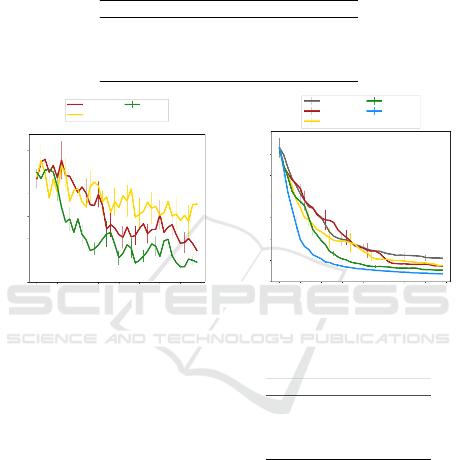
Table 2: Tested algorithms.

Name AL IRL MT

RANDOM - - Random

NOAL Random Interactive-MCE DSR

UNMOD Active-VaR MCE-IRL DSR

TLIMF Interactive-VaR Interactive-MCE DSR

TUNLIMF Not needed Not needed DSR

0 5 10 15 20 25 30 35 40

Iteration

Teacher’s loss

NOAL

UNMOD

TLIMF

(a) Teacher’s inferred policy loss.

0 5 10 15 20 25 30 35 40

Iteration

Learner’s loss

RANDOM

NOAL

UNMOD

TLIMF

TUNLIMF

(b) Learner’s policy loss.

Figure 3: Teaching results are measured as (a) the loss of the teacher’s inferred policy and (b) the loss of the actual learner’s

policy. The thick lines represent the averages of 16 experiments. The thin vertical lines measure the standard error. TLIMF

demonstrates the lowest losses during most of the process, with NOAL and UNMOD signiﬁcantly lagging behind.

teacher performs worse than TLIMF but better than

the lower baseline, RANDOM: its loss is considerably

lower starting from the 25th iteration, and it needs

fewer iterations to reach the loss thresholds. This im-

plies that teaching without AL is still better than se-

lecting demonstrations randomly. Finally, the perfor-

mance of the teacher with unmodiﬁed AL and IRL

algorithms, UNMOD, is high during the ﬁrst six iter-

ations, but it gradually worsens during the teaching

process and falls below the performance of NOAL.

It also shows signiﬁcantly low performance at reach-

ing the loss thresholds, needing more iterations than

the random teacher, which implies that modifying the

algorithms was necessary for good performance.

6 SUMMARY AND FUTURE

WORK

We have proposed a teacher-learner interaction frame-

work in which the feedback from the learner is limited

Table 3: Iterations needed to reach a loss threshold ε.

Teacher ε = 2 ε = 1 ε = 0.5

RANDOM 16 36 96

NOAL 13 25 49

UNMOD 31 54 102

TLIMF 8 19 46

TUNLIMF 5 11 27

to just one trajectory per teaching iteration. Such a

framework is closer to real-life situations and more

challenging when compared with the frameworks

used in previous works. In this framework, the teacher

has to solve AL, IRL, and MT problems sequentially

at every teaching iteration. We have proposed a teach-

ing algorithm that consists of three modules, each

dedicated to solving one of these three sub-problems.

This algorithm uses a modiﬁed MCE-IRL algorithm

for solving the IRL sub-problem, a modiﬁed Active-

VaR algorithm for solving the AL problem, and the

DSR algorithm for solving the MT problem. We have

tested the algorithm on a synthetic car-driving envi-

Interactively Teaching an Inverse Reinforcement Learner with Limited Feedback

ronment and compared it with the existing algorithms

and the worst-case baseline. We have concluded that

the new algorithm is effective at solving the teaching

problem.

In future work, it would be interesting to study

such a teacher-learner interaction in more complex

environments. For example, an environment could

have more states and a non-linear reward function

possibly represented as a neural network. Another

question yet to be addressed is the convergence guar-

antees of the proposed algorithms. It is also interest-

ing to check whether the MT module of the algorithm

could be improved by considering the uncertainty of

the estimated learner policy. Another possible direc-

tion of research is ﬁnding more sophisticated ways

of weighing older trajectories of the learner. E.g., if

the environment consists of several isolated regions

and any feature is conﬁned to a certain region, then

sending a teaching demonstration in one region might

not change the learner’s behavior in others, therefore

the previous learner’s trajectories from other regions

might not need to be weighed down.

ACKNOWLEDGEMENTS

This work was partially supported by national funds

through Fundac¸

ao para a Ci

encia e a Tecnologia,

under project UIDB/50021/2020 (INESC-ID multi-

annual funding) and the RELEvaNT project, with ref-

erence PTDC/CCI-COM/5060/2021.

Rustam Zayanov would also like to thank Open

Philanthropy for their scholarship, which facilitated

his dedicated involvement in this project.

REFERENCES

Abbeel, P. and Ng, A. Y. (2004). Apprenticeship learning

via inverse reinforcement learning. In Proceedings of

the twenty-ﬁrst international conference on Machine

learning, page 1.

Brown, D. S., Cui, Y., and Niekum, S. (2018). Risk-aware

active inverse reinforcement learning. In Conference

on Robot Learning, pages 362–372. PMLR.

Brown, D. S. and Niekum, S. (2019). Machine teaching for

inverse reinforcement learning: Algorithms and appli-

cations. In Proceedings of the AAAI Conference on

Artiﬁcial Intelligence, volume 33, pages 7749–7758.

Cakmak, M. and Lopes, M. (2012). Algorithmic and human

teaching of sequential decision tasks. In Twenty-Sixth

AAAI Conference on Artiﬁcial Intelligence.

Kamalaruban, P., Devidze, R., Cevher, V., and Singla,

A. (2019). Interactive teaching algorithms for

inverse reinforcement learning. arXiv preprint

arXiv:1905.11867.

Liu, W., Dai, B., Humayun, A., Tay, C., Yu, C., Smith,

L. B., Rehg, J. M., and Song, L. (2017). Iterative ma-

chine teaching. In International Conference on Ma-

chine Learning, pages 2149–2158. PMLR.

Liu, W., Dai, B., Li, X., Liu, Z., Rehg, J., and Song, L.

(2018). Towards black-box iterative machine teach-

ing. In International Conference on Machine Learn-

ing, pages 3141–3149. PMLR.

Lopes, M., Melo, F., and Montesano, L. (2009). Ac-

tive learning for reward estimation in inverse rein-

forcement learning. In Joint European Conference

on Machine Learning and Knowledge Discovery in

Databases, pages 31–46. Springer.

Melo, F. S., Guerra, C., and Lopes, M. (2018). Interactive

optimal teaching with unknown learners. In IJCAI,

pages 2567–2573.

Ng, A. Y., Russell, S., et al. (2000). Algorithms for inverse

reinforcement learning. In Icml, volume 1, page 2.

Settles, B. (2009). Active learning literature survey. Com-

puter Sciences Technical Report 1648, University of

Wisconsin–Madison.

Sutton, R. S. and Barto, A. G. (2018). Reinforcement learn-

ing: An introduction. MIT press.

Yengera, G., Devidze, R., Kamalaruban, P., and Singla, A.

(2021). Curriculum design for teaching via demon-

strations: Theory and applications. Advances in

Neural Information Processing Systems, 34:10496–

10509.

Zhu, X. (2015). Machine teaching: An inverse problem

to machine learning and an approach toward optimal

education. In Proceedings of the AAAI Conference on

Artiﬁcial Intelligence, volume 29.

Zhu, X., Singla, A., Zilles, S., and Rafferty, A. N. (2018).

An overview of machine teaching. arXiv preprint

arXiv:1801.05927.

Ziebart, B. D. (2010). Modeling purposeful adaptive be-

havior with the principle of maximum causal entropy.

Carnegie Mellon University.

Ziebart, B. D., Bagnell, J. A., and Dey, A. K. (2013). The

principle of maximum causal entropy for estimating

interacting processes. IEEE Transactions on Informa-

tion Theory, 59(4):1966–1980.

ICAART 2024 - 16th International Conference on Agents and Artiﬁcial Intelligence