Naval Fleet Schedule Optimization Using an Integer Linear Program

Megan Widmer

, Mich

ele Fee

and Franc¸ois-Alex Bourque

Defence Research and Development Canada, Centre for Operational Research and Analysis,

Keywords:

Schedule, Fleet, Integer Linear Program, Optimization.

Abstract:

To inform decisions about future ﬂeet planning, a way to model asset availability over time is needed. To

accomplish this, a tool was developed that generates optimized ﬂeet schedules from simpliﬁed operations and

maintenance cycles. By repeating these cycles and offsetting them from asset to asset, it is possible to generate

schedules that meet a set of ﬂeet availability requirements. Target schedule characteristics were encoded in an

Integer Linear Program (ILP) and solved using the PuLP python package with the COIN-OR branch and cut

solver. To evaluate the effectiveness of the approach, ﬂeet schedules for notional asset ﬂeets were generated

and compared qualitatively to those made using a genetic algorithm (GA) based tool that is currently in use.

The ILP tool was found to produce schedules that met the requirements more consistently than the GA.

1 INTRODUCTION

Understanding when assets in a ﬂeet are available

is a fundamental component in future ﬂeet planning.

A method that models optimized ﬂeet schedules that

conform to a set of requirements is therefore essen-

tial. Such schedules are used, for example, to inform

ﬂeet size required to meet operational ambitions and

high-level ﬂeet crewing and training requirements.

Due to the nature of the operational demand and

the logistics of ship maintenance, the ﬂeet schedules

are modelled from repeating operations and mainte-

nance cycles (OPCYCLEs), which differ from class

to class according to the assets’ maintenance require-

ments and crewing limitations. These cycles track

when each asset is available to perform operations

and by offsetting the start of each cycle from asset-

to-asset, it is possible to generate ﬂeet schedules that

meet a set of availability objectives.

The optimization of this kind of periodic or cyclic

schedule is common to a range of ﬁelds, including

medical (Ferrand et al., 2011; Burke et al., 2004)

and military applications (Verhoeff et al., 2015; Raf-

fensperger and Schrage, 1997) to track personnel and

equipment availability. In these applications, the use

of regular, repeating cyclic patterns to track overall

availability lends a predictability to the ﬁnal sched-

ule that is beneﬁcial in the context of operations plan-

https://orcid.org/0009-0005-1378-8532

https://orcid.org/0000-0002-6971-7689

ning. Optimizing schedules built from these cyclic

patterns has been done with a range of approaches, in-

cluding heuristic methods (Fee et al., 2019) and math-

ematical optimization (Ferrand et al., 2011; Verho-

eff et al., 2015). In particular the use of linear pro-

grams is well documented (Ferrand et al., 2011; Ver-

hoeff et al., 2015) since the requirements can often

be expressed in terms of linear constraints. Solutions

are often formulated as a mix of hard and soft con-

straints, where hard constraints are used to capture

requirements and restrictions, while soft constraints

capture preferences. A hard constraint describes a

scenario where a solution is not feasible if that con-

straint cannot be met, such as was used with Deris

et al. (1997) with maintenance requirements. A soft

constraint uses a slack variable that tracks a penalty

when the constraint is not found, but which is help-

ful in solving schedules with some ﬂexibility of the

outcome. Ferrand et al. (2011) for example uses

both hard and soft constraints in optimizing physi-

cian work schedules, where the hard constraints are

the work requirements, and the soft constraints are

the physicians work preferences. Integer Linear Pro-

gram (ILP) was chosen to perform the optimization in

this work because heuristic methods do not guarantee

identiﬁcation of a global optimum and can be difﬁcult

to tune. The ILP tool uses a combination of hard and

soft linear constraints to bind a solution space and an

objective function to determine the optimal arrange-

ment of each asset’s cycles in relation to each other.

Widmer, M., Fee, M. and Bourque, F.

Naval Fleet Schedule Optimization Using an Integer Linear Program.

DOI: 10.5220/0012272200003639

Paper copyright by his Majesty the King in Right of Canada as represented by the Minister of National Defence

In Proceedings of the 13th International Conference on Operations Research and Enterprise Systems (ICORES 2024), pages 47-57

ISBN: 978-989-758-681-1; ISSN: 2184-4372

The ILP tool was built using the PULP Python

package (Foundation, 2023). The objective for the

tool was to create optimized schedules for single- or

multi-class ﬂeets at a steady state of operations. The

constraints were developed to be modular in order to

be easily adapted to account for a range of different

availability requirements, including those that arise

from a ﬂeet split across separate home ports, as was

demonstrated here. To evaluate the effectiveness of

the tool, ﬂeet schedules were generated for asset ﬂeets

with notional maintenance cycles. These will be com-

pared qualitatively to those produced using a genetic

algorithm-based ﬂeet optimizer (Fee et al., 2019) that

is currently in use to support navy planning.

2 METHODOLOGY

To generate ﬂeet schedules, an operations and mainte-

nance cycle, or OPCYCLE, is used as the main build-

ing block. These provide a semi-ﬂexible mapping

of the asset’s readiness states over time. An asset’s

readiness state is the measure of its availability to per-

form operations. The schedule for a single asset is

made by repeating the OPCYCLE sequence over a

span of time. By choosing the offset between each as-

set schedule within a ﬂeet, it is possible to distribute

available and unavailable states across the ﬂeet sched-

ule to meet a set of requirements.

2.1 OPCYCLE and Readiness States

For the purposes of this report, the following readi-

ness states are used:

• Extended Readiness (ER): The asset is in deep

maintenance (usually in dry dock), so it is not con-

sidered employable and is not normally crewed.

• Restricted Readiness (RR): In this readiness state,

the asset is in shallow maintenance.

• Normal Readiness (NR): This is a period when the

asset can conduct limited domestic operations.

• High Readiness (HR): This is a period when the

asset is in the highest state of readiness and so it

can deploy on expeditionary operations and con-

duct the full spectrum of combat operations;

Each readiness state involves a different level of crew

training as well as availability of different equipment

on board. Remaining at the highest state of readiness

is taxing on both the crew and the asset and so can

only be maintained for a speciﬁc number of months.

Figure 1 shows an example of a typical OPCY-

CLE. Each block represents a time period where the

asset is at a particular readiness state and this se-

quence shows the transition from lowest readiness to

highest and back again.

Each asset starts in deep maintenance (ER) and

then begins its trajectory towards higher readiness

states. To start preparing the asset for operations, it

undergoes an intermediate RR stage. Once the asset

is out of the RR state, it will be at NR by default and

may be raised to HR at any time before the next ER

or RR period, whichever is ﬁrst. Once the HR deploy-

ment is completed, the asset will either return to NR

or, if it is due for maintenance, enter the scheduled

ER or RR period.

2.1.1 OPCYCLE Repeats

If the schedule length is longer than the OPCYCLE,

the cycle is repeated. For example, for the OPCY-

CLE described in Figure 1, to generate a schedule of

30 time units long, the OPCYCLE would be repeated

twice. If the schedule length is not a multiple of the

length of the OPCYCLE, as shown in Figure 2 for

a ﬂeet schedule of 20 time steps, partial OPCYCLE

repeats are used. Any time steps beyond t=19 are ig-

nored.

2.1.2 Sub-Operational Cycles

Since it is taxing on both the equipment and the crew

to maintain an asset at a higher state of readiness for

long periods of time, the operational cycles are often

broken up into smaller sub-segments, referred to here

as sub-OPCYLEs. Each sub-cycle contains a single

HR period and is delineated by short, shallow main-

tenance periods rather than the longer, deep mainte-

nance found at the start of the cycle.

Each sub-OPCYCLE includes a single sequence

of RR, NR, and HR readiness states, where the time

that the asset spends at NR and/or HR as well as the

placement of the HR state may vary. In Figure 3, the

two sub-OPCYCLEs are labelled.

2.1.3 Placement of the HR State

Following the RR stage in each sub-OPCYCLE, the

asset may enter the HR state or transition to NR. Once

at NR, the asset may be raised to HR at any time be-

fore the start of the next maintenance period (ER or

RR). In Figure 4, the ﬁrst sub-OPCYCLE of the OP-

CYCLE from Figure 1 is examined. In Panel (a), the

HR state starts after the RR state ends, while in Panel

(b), (c) and (d), the start of the HR period is offset by

one, two and three time steps respectively.

For example, in Figure 1, the length of the HR

offset in the ﬁrst sub-OPCYCLE is zero (directly af-

ter the RR period) and in the second sub-OPCYCLE

ICORES 2024 - 13th International Conference on Operations Research and Enterprise Systems

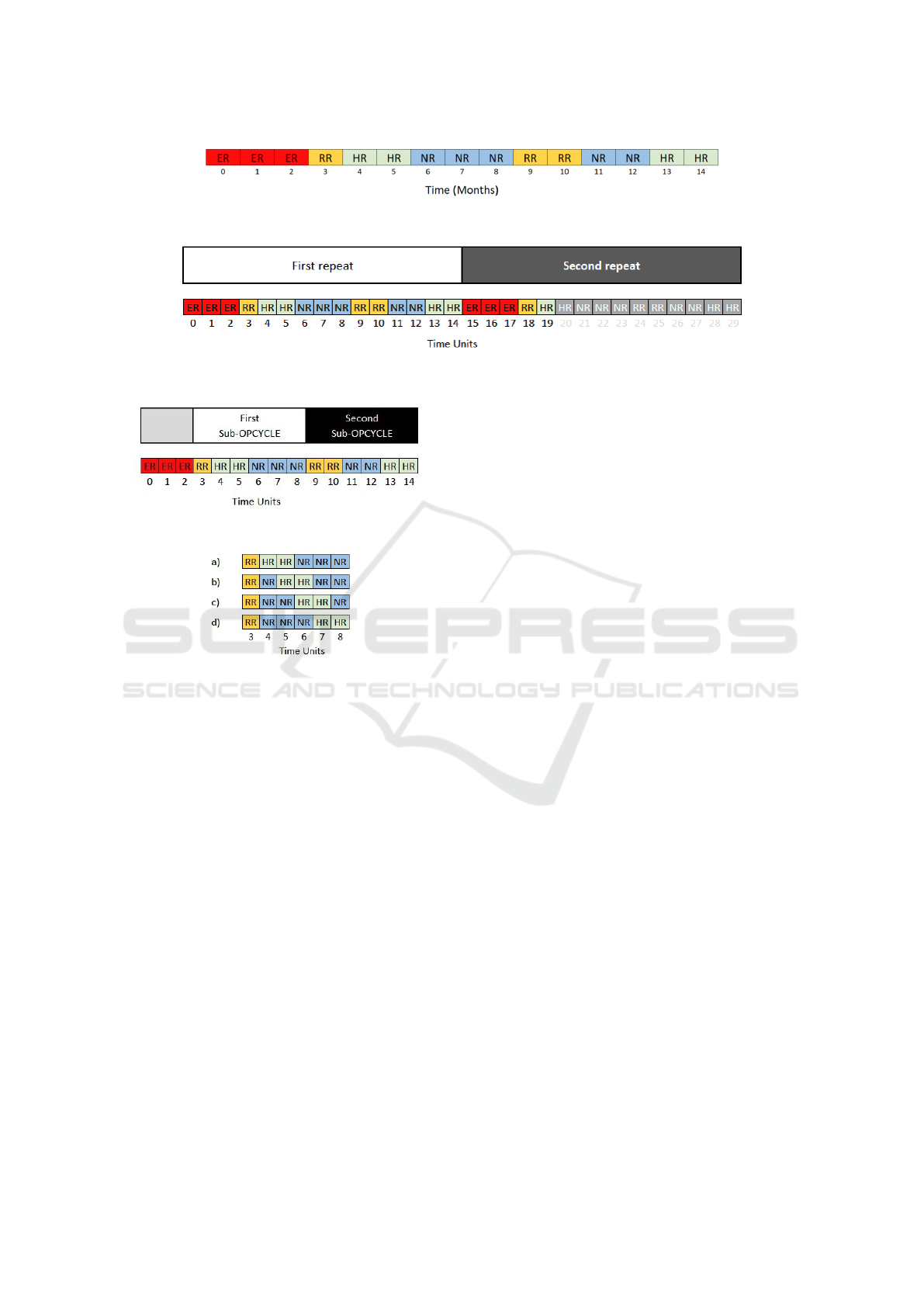
Figure 1: Notional example of an OPCYCLE.

Figure 2: An illustration on how the repeats of an OPCYCLE work using a ﬂeet schedule of 20 time units. The gray readiness

states that begin at t = 20 show those outside the ﬂeet schedule.

Figure 3: Illustration of sub-OPCYCLEs.

Figure 4: Examples of HR period offset.

is two (two blocks away from the RR period). Break-

ing the OPCYCLE up in this way allows for the in-

dependent placement of the HR period in each sub-

OPCYCLE, as seen in Figure 1, which will be an inte-

gral part of the subsequent formulation since the ﬂexi-

bility allows readiness requirements to be more easily

met.

2.1.4 Wrap Around Feature

For a schedule at steady state, when an OPCYCLE is

offset from asset-to-asset, it is necessary for the OP-

CYCLE to wrap around to the start. For example,

in Figure 5, a single asset schedule of 20 time units

made from the OPCYCLE in Figure 1 is offset by 5

time units (the ER block begins at 5). The ﬁrst OP-

CYCLE runs from time step 5 to 19, and then repeats

from time step 20 to 29. The last 5 blocks of that sec-

ond OPCYCLE wrap around to the beginning of the

schedule and appear in time steps 0 through 4 of the

schedule (labeled as “second repeat”).

2.2 Fleet Schedule

Combining individual asset schedules, it is possible

to construct a ﬂeet schedule, such as that shown in

Figure 6. In this representation of a ﬂeet schedule,

each row represents a single asset schedule where the

coloured tiles represent the readiness states. This ﬁg-

ure shows an example of a ﬂeet schedule for a no-

tional ﬂeet of ﬁve assets using the OPCYCLE de-

scribed in Figure 1. To the right of the ﬂeet schedule

is a table showing the offset of each asset schedule.

2.2.1 Sub-Fleets

Occasionally it is necessary to track readiness states

by grouping of assets, such as those with a common

home port or those within a larger ﬂeet belonging to

different classes of asset. To accommodate this, the

tool includes the idea of sub-ﬂeets. For example using

Figure 6, the ﬂeet of ﬁve assets can be split between

two different sub ﬂeets, Port A and Port B. For the

notional example, assets 0-2 are based in Port A and

assets 3-4 are based in Port B. So, the ﬂeet schedule

now has two sub-ﬂeets that can have their own opti-

mization objectives.

2.3 Characteristics of a Good Schedule

In a naval context, there are many distinct character-

istics that make up a good, optimized schedule. They

are:

1. A consistent number of assets at ER for all assets

at each time unit;

2. A consistent number of assets at HR for all assets

at each time unit; and

3. A consistent number of assets at HR for the assets

in each sub-ﬂeet.

While the structure length and placement of the ER

periods in the OPCYCLE captures the assets’ main-

Naval Fleet Schedule Optimization Using an Integer Linear Program

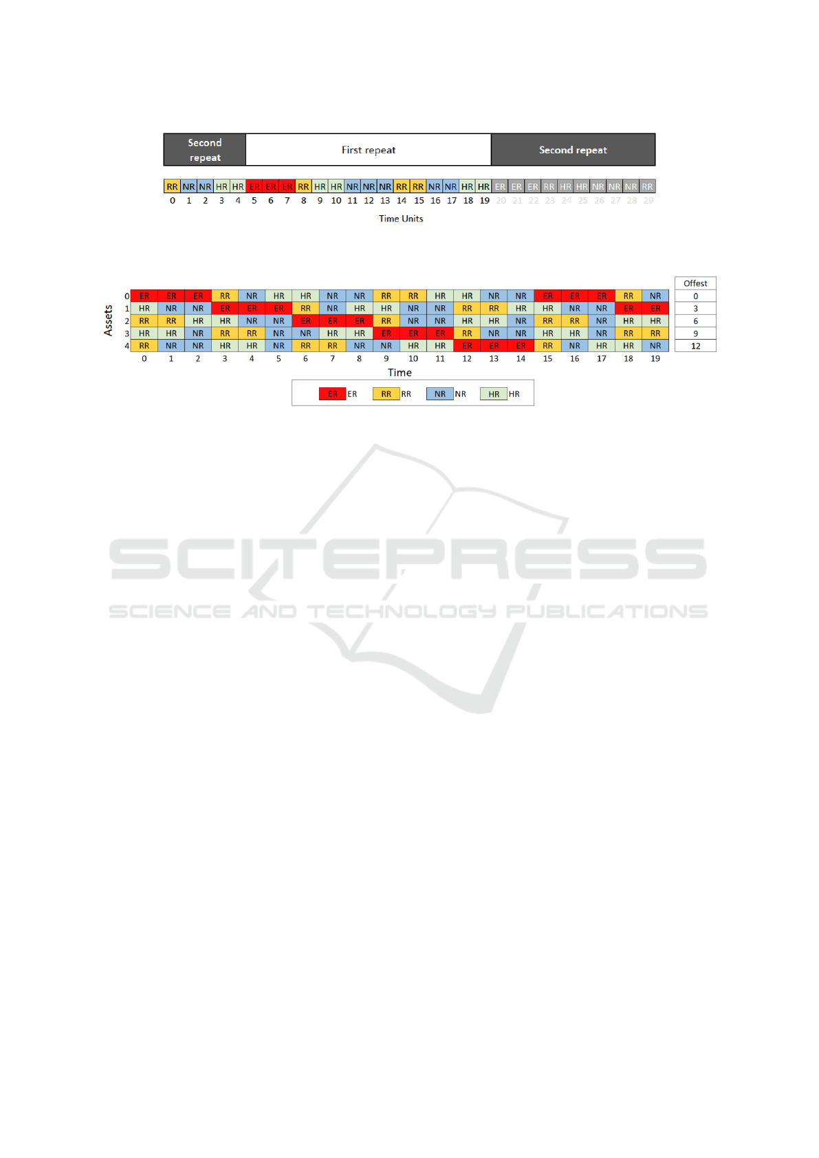
Figure 5: A demonstration of the wrap around feature of an OPCYCLE that has an offset of 5 time units. The gray readiness

states that begin at time step 20 show those outside of the ﬂeet schedule.

Figure 6: Fleet schedule for ﬁve assets spanning 20 time units.

tenance needs, this consistency needed for at the

schedule-level stems from the maintenance facility’s

workload balancing requirements. If there are mul-

tiple maintenance facilities for a given ﬂeet of assets,

this ﬁrst characteristic is imposed at the sub-ﬂeet level

rather than for all the assets.

The second and third characteristics are derived

from the underlying operational demand that the asset

ﬂeet is expected to fulﬁl. With the exception of ﬂeets

tied to speciﬁc seasonal operations, the bulk of the

operational demand is across the ﬂeet as well as at the

sub-ﬂeet level is consistent throughout the year. As a

result, an attempt is made to maintain the number of

assets at

HR consistent over time in the whole ﬂeet as

well as each sub-ﬂeet.

These three characteristics are included in the con-

straints used in the mathematical formulation of the

ﬂeet scheduling problem.

2.4 Integer Linear Program

The following section describes the implementation

of the integer linear program (ILP) used to optimize

ﬂeet schedules.

2.4.1 Indices

Below are all of the indices used in the formulation of

the ILP tool.

i a sub-ﬂeet

a an asset

t a time step

k an OPCYCLE offset

h an OPCYCLE repeat

d a sub-OPCYCLE

l a HR period offset

2.4.2 Sets

Below are all of the sets used in the formulation of the

ILP.

I the set indexing the sub-ﬂeets

A the set indexing the whole ﬂeet of assets

the set indexing the assets in sub-ﬂeet i

T the set of time steps

K the set of possible values by which an

OPCYCLE is offset relative to the start

of the ﬂeet schedule

the set indexing the OPCYCLE repeats

of asset a in the ﬂeet schedule

a,h

the set indexing the sub-OPCYCLEs of

asset a and for each OPCYCLE repeat h

a,h,d

the set of possible values by which a HR

period is offset relative to the RR period

of sub-OPCYCLE d for each OPCYCLE

repeat h and for each asset a

The ﬂeet schedule from Figure 6 can be used to better

interpret the sets and indices deﬁned. Starting with

the set T that represents the 20 time steps that make

up the schedule length that can be represented as T =

{0, ..., 19}.

The ﬁve assets in Figure 6 are represented by the

set A = {0, 1, 2, 3, 4}. The set I represents the whole

ICORES 2024 - 13th International Conference on Operations Research and Enterprise Systems

ﬂeet (indicated by zero) and two sub-ﬂeets that cor-

respond to Port A (indicated by one) and Port B (in-

dicated by two), so the set is I = {0, 1, 2}. There are

three sets for A

the total ﬂeet A

= A for the Port A,

= {0, 1, 2} and for the Port B, A

= {3, 4}.

The set K has 20 possible OPCYCLE offset

starting points which can be represented as K =

{0, ..., 19}. Since the OPCYCLE is 15 time units long

and the ﬂeet schedule is 20 time units long, there are

two repeats of the OPCYCLE represented by the set

. The ﬁrst repeat is full and the second repeat

slightly shortened, and depending on the offset the

formulation will remove the excess time steps after

the offset has been applied. Since the ﬂeet schedule

only contains one OPCYCLE and each asset has the

same number of repeats, H

= {0, 1}, ∀ a. In this set,

zero represents the portion of the ﬂeet schedule shown

as the “ﬁrst repeat” in Figures 2 and 5 and one as the

“second repeat” in those ﬁgures.

Similarly, from Figure 1, there are two sub-

OPCYCLEs that are present and since each asset has

the same OPCYCLE, D

a,h

= {0, 1}, ∀ a and h. For

this example, the sub-OPCYCLE indicated by zero

includes the potions highlighted in Figure 4 (t = 3

to t = 8 in the OPCYCLE). The D

a,h

= 1 refers to

the second sub-OPCYCLE between t = 9 to t = 14 in

Figure 1.

Finally, the set L

a,h,d

represents the possible rela-

tive offset of each HR. Using the OPCYCLE in Fig-

ure 1, the set L

a,h,d

, ∀ a and h can be determined.

The single OPCYCLE contains two sub-OPCYCLEs

so there are two sets for both values of d:

a,h,d

(

{0, 1, 2, 3, 4} if d = 0

{0, 1, 2, 3} if d = 1

The positions for the ﬁrst sub-OPCYCLE (d = 0)

1, 2, 3 and 4 are shown in Figure 4. Since the sec-

ond sub-OPCYCLE (d = 1) is shorter, there are fewer

permissible values for L

a,h,d

2.4.3 Variables

Below are the variables used in the formulation of the

ILP.

(a)

a binary variable that indicates

whether the OPCYCLE starts at the

time step t = k. For example, in Fig-

ure 6, since the OPCYCLE for asset

1 begins at t = 3, X

(0)

= 1, X

(0)

= ...X

(0)

= 0.

(a,h,d,l)

a binary variable that indicates

whether the HR period for each sub-

OPCYCLE, d, and each repeat of

the OPCYCLE in the ﬂeet schedule,

h, is shifted by l time steps from

the start of the availability block.

In Figure 6, for asset 2 (counting

from the start of the OPCYCLE at

t = 6), the visible HR periods are

shifted by 2, 1 and 0. As a result,

(2,6,0,0)

(2,6,0,1)

(2,6,1,1)

=0. The

HR block at h = 1,d = 0 is not shown

since it occurs between t = 20 and

t = 29 and is trimmed off.

a binary slack variable that counts

how many time step have soft con-

straints that are not met over the time

period of the ﬂeet schedule.

2.4.4 Parameters

Below are the parameters used in the formulation of

the ILP tool.

(a)

t,k

a matrix indicating when asset a is at

ER. It returns one if asset a is at ER at

time step t given that its OPCYCLE

is offset by k, otherwise it returns to

zero.

(a,h,d,l)

t,k

a matrix indicating when asset a is at

HR. For an OPCYCLE offset by k,

it returns one when asset a is at HR

at time step t for each HR period in

sub-cycle d of OPCYCLE repeat h

for each offset of l, otherwise it re-

turns zero.

M the large integer used with the slack

variables

MaxER

the maximum quantity of assets at

ER for each sub-ﬂeet i

MaxHR

the maximum quantity of assets at

HR for each sub-ﬂeet i

MinER

the minimum quantity of assets at ER

for each sub-ﬂeet i

MinHR

the minimum quantity of assets at HR

for each sub-ﬂeet i

For the notional example of Figure 1, since the OP-

CYCLEs are identical for all assets, the matrices

(a)

t,k

are the same for all assets. In other words,

(0)

t,k

=ER

(1)

t,k

=...=ER

(4)

t,k

, shown in Figure 7.

In this matrix, a value of one corresponds to the

presence of an ER block at a particular time step, t,

(row) given a particular offset, k (column). Since each

asset can only have one such offset (only one value of

k), this matrix is used in the constraints described in

Naval Fleet Schedule Optimization Using an Integer Linear Program







1 0 0 ·· · 1 1

1 1 0 ·· · 0 1

1 1 1 ·· · 0 0

0 1 1 ·· · 0 0

0 0 1 ·· · 0 0

0 0 0 ·· · 0 0

0 0 0 ·· · 1 0

0 0 0 ·· · 1 1

1 0 0 ·· · 1 1

1 1 0 ·· · 0 1

1 1 1 ·· · 0 0

0 1 1 ·· · 0 0

0 0 1 ·· · 0 0







Figure 7: Matrix ER

(a)

t,k

for the notional OPCYCLE shown

in Figure 1.

subsection 2.4.5 to track the total number of assets in

the ER state.

Figure 8 show an example matrix for HR

(a,h,d,l)

t,k

As with the ER

(a)

t,k

, these values are OPCYCLE-

dependent and so the matrices is the same for all as-

sets in the notional example. The matrix shown below

is for the ﬁrst repeat of the OPCYCLE (h = 0) and

correspond to the positioning of the HR period in the

ﬁrst repeat (d = 0) where it is not shifted from the end

of the maintenance period(l = 0).

As k is increased (in the matrix, moving to the

right), the time step at which the HR states occur is

shufﬂed forward in time and, accordingly, down the

rows of the matrix.

In Figure 8, the ﬁrst two matrices represent the

ﬁrst HR period in the OPCYCLE. As l is increased,

as for Figure 8 (a) to (b), the position of the ones,

are shifted forward in time or downward in the ma-

trix. The matrices in Figure 8 (c) and (d) represent

this mapping for the second sub-OPCYCLE and so

the ones start further down in the matrix.

The value of M was chosen to be 100 since it much

larger than the ﬂeet sizes that are expected to be used

with this tool.

In the notional example provided in Figure 1, the

maximum number of assets at ER for each sub-ﬂeet,

designated by the variable MaxER

, was calculated

using Eq. (1).







0 0 ·· · 0 0

1 0 ·· · 0 0

1 1 ·· · 0 0

0 1 ·· · 0 0

0 0 ·· · 0 0

0 0 ·· · 1 0

0 0 ·· · 1 1

0 0 ·· · 0 1







Figure 8: Example matrices for HR

(a,0,0,0)

t,k

MaxER



ER in OPCYCLE

Length of OPCYCLE

×Number of Assets

(1)

To keep the number of assets close to this maxi-

mum bound, the minimum bound for the number of

assets at ER for each sub-ﬂeet, M inER

, was set to

one fewer than the MaxER

Using the notional example for a ﬂeet schedule of

length t = 15 that was used to calculate MaxER

the

maximum number of assets for each sub-ﬂeet can be

calculated using Eq. (1).

MaxER



× 3





× 2



0.6 + 0.4

= 1.0

MaxER



× 3



0.6

= 1.0

MaxER



× 2



0.4

= 1.0

(2)

MaxER

must have a minimum value of one and

so the value for both sub-ﬂeets, MaxER

and MaxER

is rounded up to one.

ICORES 2024 - 13th International Conference on Operations Research and Enterprise Systems

A similar calculation, shown in Eq. (3), can be

conducted to determine the maximum number of as-

sets at HR for each sub-ﬂeet, designated by the vari-

able MaxHR

MaxHR



HR in OPCYCLE

Length of OPCYCLE

×Number of Assets

(3)

The minimum number of assets at HR for each

sub-ﬂeet, MinHR

, was calculated using the value of

MaxHR

MinHR

= MaxHR

− 1 (4)

Using the notional example for a ﬂeet schedule of

length t = 15 with ﬁve assets, three in one sub-ﬂeet

and two in the other, the maximum number of assets

for each sub-ﬂeet can be calculated using Eq. (3).

MaxHR



× 3





× 2



0.8 + 0.5333

1.3333

= 2.0

MaxHR



× 3



0.8

= 1.0

MaxHR



× 2



0.5333

= 1.0

The result was one for both sub-ﬂeets, which

means that a maximum of one asset for each sub-ﬂeet

can be at HR at any time unit.

2.4.5 Constraints

Below are all of the constraints that were used in the

formulation of the ILP tool.

First Offset is Zero

The ﬁrst constraint is used to force the ﬁrst asset in

the ﬂeet schedule to start the ER at the ﬁrst time unit.

(0)

= 1 (5)

All Assets Must Only Have One Assigned Offset

This constraint is used to tell the model that, for each

asset, there can only be one starting point for the OP-

CYCLE.

∑

k∈K

(a)

= 1 ∀a ∈ A (6)

From the notional example in Figure 6, for each asset

in the schedule a constraint is produced, so there are

six constraints. The ﬁrst one is:

(0)

+ X

(0)

+ X

(0)

+ X

(0)

+ X

(0)

= 1

Bounding the Number of Assets at ER

For the sub-ﬂeets deﬁned by A

, the number of assets

in ER is bound between MaxER

and MinER

∑

a∈A

∑

k∈K

(a)

t,k

≤ MaxER

∀i ∈ I and t ∈ T

(7)

∑

a∈A

∑

k∈K

(a)

t,k

≥ MinER

∀i ∈ I and t ∈ T

(8)

From the notional example in Figure 1, consider

the whole ﬂeet A

= {0, 1, 2, 3, 4}. There are a total of

40 constraints. Set MaxER

and MinER

to 1 and 0,

respectively, the ﬁrst constraints of Equations (7) and

(8) are written as

0 ≤ X

(0)

+ X

(0)

+ X

(a)

+ . . . + X

(4)

+ X

(4)

+ X

(4)

≤ 1

Bounding the Number of Assets at HR

For the sub-ﬂeets deﬁned by A

, the number of assets

in HR is bound between MaxHR

and MinHR

. A

slack variable, Z

, is introduced at each time unit t to

soften the constraints yielding:

− (MZ

∑

a∈A

∑

k∈K

∑

h∈H

∑

d∈D

a,h

∑

l∈L

a,h,d

(a,h,d,l)

t,k

≤ MaxHR

∀i ∈ I and t ∈ T (9)

(MZ

∑

a∈A

∑

k∈K

∑

h∈H

∑

d∈D

a,h

∑

l∈L

a,h,d

(a,h,d,l)

(a)

t,k,h,d,l

≥ MinHR

∀i ∈ I and t ∈ T (10)

The big-M method was selected for these con-

straints to simplify the problem. While it is possi-

ble to exclude the big-M and use the slack variable to

track the deviation of the number of assets at HR from

the HRMax

and HRMin

, this requires a Z variable

for each constraint rather than each time step. Link-

ing the slack variable across several constraints does

run the risk of permitting more constraints to be bro-

ken for a given timestep without penalty as soon as

one was broken, but this was not found to be the case

with the scenarios tested. This is likely because of

Naval Fleet Schedule Optimization Using an Integer Linear Program

the way the HRMax

and HRMin

range was calcu-

lated paired with the ﬂexibility given to the HR place-

ment within the sub-OPCYCLEs. This meant these

soft constraints were generally easy to meet.

From the notional example in Figure 1. For

the sub-ﬂeet containing all assets, A

= {0, 1, 2, 3, 4},

the constraint equations produced a total of 40 con-

straints. Setting MaxHR

and MinHR

to be two and

one respectively, the ﬁrst constraint of Equations (9)

and (10), where t = 0, are written as:

1 ≤ Y

(0,1,1,2)

(0,1,1,1)

(0,1,1,2)

(0,1,1,0)

(0,1,1,1)

(0,1,1,0)

(0,1,0,3)

(0,1,0,2)

(0,1,0,3)

(0,1,0,1)

(0,1,0,2)

(0,1,0,0)

(0,1,0,1)

(0,1,0,0)

+ . . . +Y

(4,1,1,2)

(4,1,1,1)

(4,1,1,2)

(4,1,1,0)

(4,1,1,1)

(4,1,1,0)

(4,1,0,3)

(4,1,0,2)

(4,1,0,3)

(4,1,0,1)

(4,1,0,2)

(4,1,0,0)

(4,1,0,1)

(4,1,0,0)

− 100Z

≤ 2 (11)

Link X and Y Variables

To ensure that the solution for X

(a)

and Y

(a,h,dl,k)

cor-

respond to the same k, the variables are linked using

the constraint shown in Equation (12).

− X

(a)

∑

l∈L

(a,h,d,l)

= 0

∀a ∈ A, k ∈ K, h ∈ H and d ∈ D (12)

This equation ensures that if the solution for

(a)

=0, then the corresponding Y

(a,h,d,l)

do not con-

tain a value of one. As written, this equation also

makes sure that, for an X

(a)

with a value of one, only

one offset l is selected for each HR period.

From the example in Figure 1, there are a total

of 60 constraints that are generated, one for each HR

period in the ﬂeet schedule. An example of the ﬁrst

constraint is provided below.

−X

(0)

(0,0,0,0)

(0,0,0,1)

(0,0,0,2)

= 0

2.4.6 Objective

The objective of the ILP, shown in Equation (13), en-

sures that the number of assets at HR for the sub-ﬂeets

in question stray minimally from the prescribed target

ranges.

minimize

∑

t∈T

|T |

(13)

2.4.7 Existing Genetic Algorithm Tool

A genetic algorithm schedule optimization tool was

developed to generate ﬂeet schedules for a navy in

transition (Fee et al., 2019). The tool was intended to

characterize the capability gap that would occur given

the time-lines involved in replacing an older ﬂeet with

a newer one. It has since been adapted to handle

steady state schedules. The cost function of the GA

included the following terms:

• Penalty for the number of times the schedule

failed to stay within a target range of number of

assets at ER.

• Penalty for how much the total number of assets

at HR at each time deviated from a target number.

• Penalty for ﬂuctuations in the total number of as-

sets at ER measured as the sum of the standard

deviation in a rolling 24-time-increment window

along the length of the schedule.

• Penalty for ﬂuctuations in the total number of as-

sets at HR measured as the sum of the standard

deviation in a rolling 24-time-increment window

along the length of the schedule.

Given the non-linear nature of the last two terms,

the GA was deemed an appropriate tool at the time.

While the schedules were deemed to be better than

one could achieve by hand, they did not always con-

form strictly to the ﬂeet availability requirements dis-

cussed above. As a result, an attempt to generate lin-

ear constraints that could produce a higher quality re-

sult was attempted with the current ILP tool.

3 RESULTS

The schedule optimization tools described above were

used to create 12-year schedules for a notional ﬂeets

with four, six, eight, ten, and 12 assets. These are used

as a basis of comparison between the GA tool and the

ILP tool to allow for a qualitative comparison between

the algorithms used. For all the ﬂeet schedules, the as-

sets are split evenly between Port A and Port B. These

make up two sub-ﬂeets in the example, each having a

distinct OPCYCLE shown in Figure 9. The two OP-

CYCLEs were very similar, but since the deep main-

tenance facilities are located at Port A, the OPCY-

CLE for assets assigned to Port B has a slightly longer

ER period to account for travel to this facility. These

12-year OPCYCLEs have three sub-OPCYCLEs each

with one HR period of 12 months each. A time unit

of one month was selected.

ICORES 2024 - 13th International Conference on Operations Research and Enterprise Systems

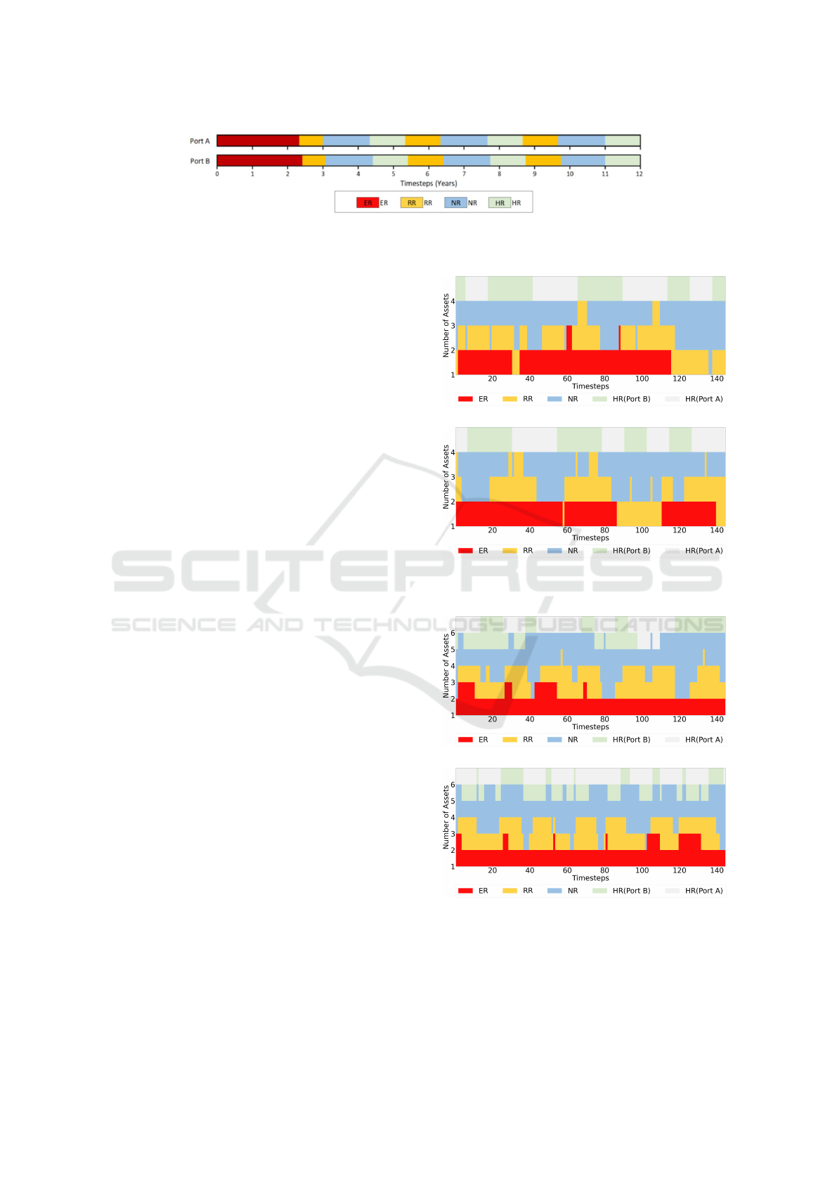
Figure 9: OPYCLEs for assets at Port A and Port B.

3.1 Evaluation of the Fleet Schedule

For the GA and the ILP, ﬂeet schedules were gen-

erated for ﬁve ﬂeet sizes (four, six, eight, ten and

twelve) using the OPCYCLEs from Figure 9. The

schedules were compared qualitatively according to

their conformity to the characteristics of a good

schedule. To facilitate this evaluation, stacked bar

graphs were generated that show the number of assets

at each readiness state for each month.

The stacked bar graphs are shown for both sched-

ules generated by the GA and ILP tools are shown in

Figure 10 to 14.

3.2 Total Assets at ER

Because of the way that the GA implemented the ER

availability schedule requirement, it had mixed suc-

cess with generating schedules where the number of

assets did not ﬂuctuate unnecessarily. The GA at-

tempted to maintain the number of assets at ER at a

particular target value, effectively MinER

, while lim-

iting variation around this target by penalizing devi-

ations from this value. This method resulted in the

number of assets at ER occasionally increasing too

high.

For example, in the six- and eight-asset ﬂeet

schedules, shown in Figure 11 and 12, the number

of assets at ER remained in a range of one assets (be-

tween one and two assets) for the whole schedule. In

the case of the solutions for the four-, ten- and twelve-

asset ﬂeets, found in Figures 10, 13 and 14, respec-

tively, the number of assets ﬂuctuated by three assets.

This is most visible in the 12-asset schedule, shown

in Figure 14(a). In this case, MaxER

is three, but the

number of assets at ER spiked to four around t = 20

and dipped down to one around t = 120. These ﬂuc-

tuations in the number of assets at ER places a strain

on the maintenance facility, requiring them to employ

and discharge staff to adapt to rapid changes in de-

mand.

By changing the way this is constrained in the ILP,

these ﬂuctuations were minimized. For all the sched-

ules produced by the ILP, the total number of assets at

ER are strictly bound between MaxER

and MinER

For example, in the ten-asset results as shown in Fig-

(a) Genetic Algorithm.

(b) Integer Linear Program.

Figure 10: Comparing the schedules of 4.

(a) Genetic Algorithm.

(b) Integer Linear Program.

Figure 11: Comparing the schedules of 6.

ure 13, for all months, the total number of assets at

ER remains at a value of one or two assets.

Naval Fleet Schedule Optimization Using an Integer Linear Program

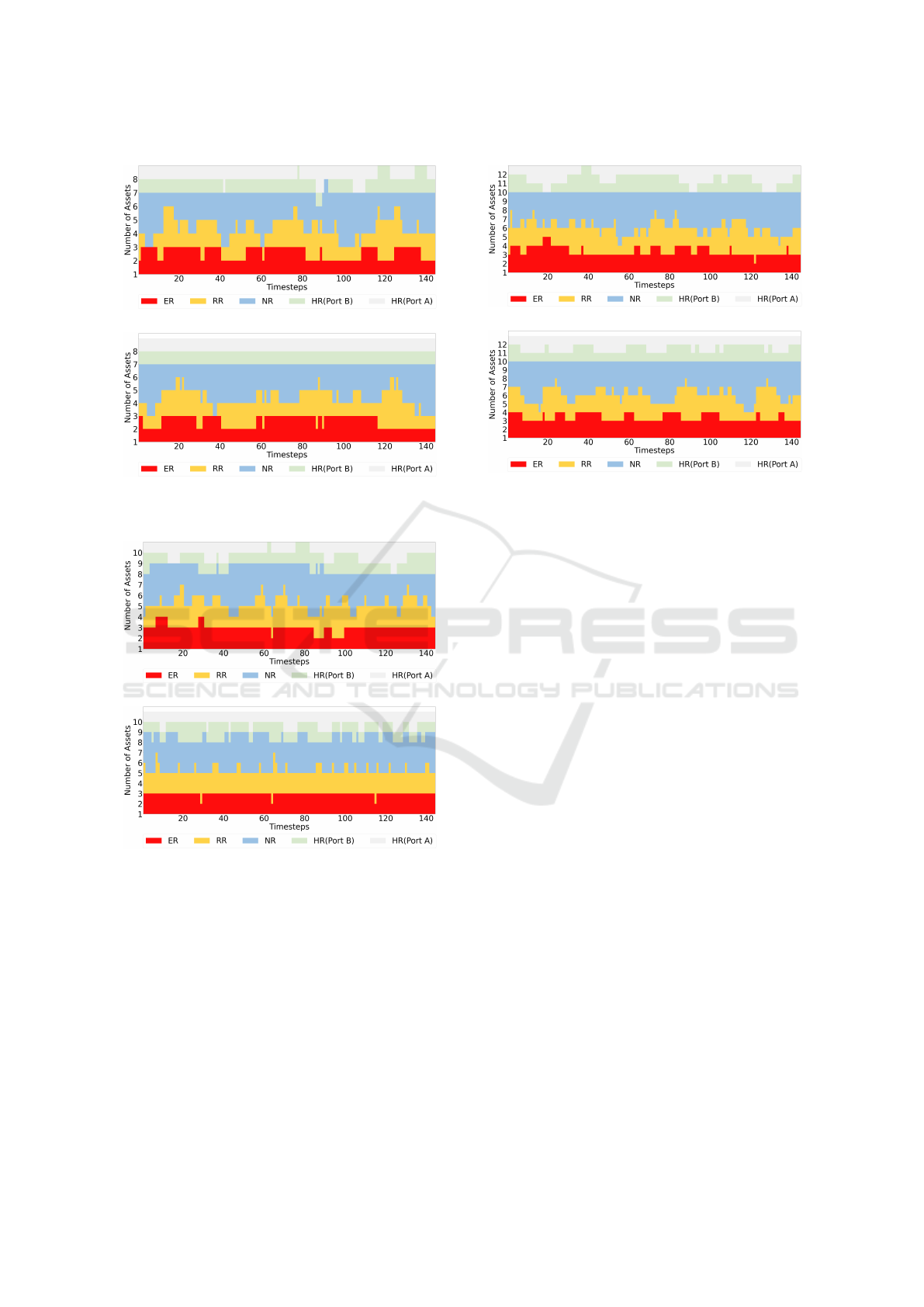
(a) Genetic Algorithm.

(b) Integer Linear Program.

Figure 12: Comparing the schedules of 8.

(a) Genetic Algorithm.

(b) Integer Linear Program.

Figure 13: Comparing the schedules of 10.

3.3 Overall Assets at HR

The overall number of assets at HR in the GA gen-

erated schedules exhibiting a similar behaviour to the

number of assets at ER. The number of assets at HR

for most schedules varied by at most one. Exception-

ally, the eight-asset ﬂeet in Figure 12 showed a minor

inconsistency, where from t = 89 to t = 91, where

there was a spike to three assets, followed by a dip to

one from t = 93 to t = 95. In this instance, it should

be possible to ﬁll the deﬁcit with the surplus that was

observed.

(a) Genetic Algorithm.

(b) Integer Linear Program.

Figure 14: Comparing the schedules of 12.

In the ILP, while the number of assets at HR in the

whole ﬂeet is encoded as a soft constraint, restrict-

ing the number between a range of acceptable values

(between MinHR

and MaxHR

) for each time incre-

ment in the schedule was as successful as it is with the

number of assets at ER. For example, it can be seen

the ten-asset result as shown in Figure 13 that the total

of assets at HR stays between values of two and three

for all months.

One side effect of the way in which the GA and

ILP handle this schedule restriction is the distribution

of the ﬂuctuations observed. In the four-, eight- and

twelve-asset ﬂeets, shown in Figure 10, 12 and 14,

respectively, it is possible to ﬁnd a solution where ex-

actly one, two and three assets, respectively, are at HR

for the entire schedule. In the six- and ten-asset ﬂeets

shown in Figure 11 and 13 where this is not the case,

the way in which the number of assets at HR cluster

is different.

In the GA tool, the ﬂuctuations are controlled by

attempting to reduce the local variability along the

schedule by incurring a penalty that is the sum of the

standard deviation of a rolling 24-step interval over

the length of the schedule.

In doing so, ﬂuctuations in the number of assets

at HR are minimized, resulting larger clusters of time

when the number of assets are higher or lower. For

example, in Figure 13, the intervals where there are

three assets at HR are grouped into roughly two clus-

ters, around t = 30 to t = 40 and t = 85 to t = 144.

In the ILP result for this same ﬂeet size, there are a

greater number of smaller groupings.

In the context of a naval ﬂeet schedule, this ob-

servation points to an important secondary character-

ICORES 2024 - 13th International Conference on Operations Research and Enterprise Systems

istic of ﬂeet schedules not taken into account in the

formulation of both tools. The frequency and dura-

tion of changes to availability would have an impact

on the operation of a ﬂeet. For the sake of longer

term planning, the regularity of availability at differ-

ent readiness states at a ﬂeet level reduces strain on

the supporting infrastructure, such as personnel and

maintenance facilities. That being said, there is also

likely an optimum duration of any increases in avail-

ability that could be leveraged. This optimum would

be dependent on the type of operations that the ﬂeet

would undertake. For example, having the equivalent

of one additional asset frequently available at HR for

one week at a time may not provide a measurable ben-

eﬁt, while having a surge of one less often, but for 4-8

months may provide an advantage.

3.4 Assets at HR by Home Port

Since the GA did not aim to control the number of as-

sets at either port in any way, it performed poorly in

this respect. Analysing each port separately revealed

schedules where the assets at HR on a coast fell to

zero at times. In the smaller ﬂeets, speciﬁcally the

four- and six-asset results, there were large periods of

time where only one coast has assets at HR. This was

inevitable since the MaxHR

and MaxHR

were less

than one for these ﬂeets. While this is unavoidable in

the smaller ﬂeets, this dip to zero assets was found to

occur in the larger ﬂeets as well. For example, in the

12-asset schedule (Figure 14) around t = 130, there

is a period of time where only the Port A has assets

at HR. The MaxHR

and MaxHR

are both two, in-

dicating that it should be feasible to maintain at least

one asset per home port at all times.

With the ILP, this restriction was added in. As

a result, the number of assets at HR in each home

port is allocated as expected: these stayed between

the ranges of MaxHR

and MinHR

(Port A) and

MaxHR

and MinHR

(Port B) at any given month.

Two good examples of this are the six- and eight-asset

ﬂeet results. The eight-asset ﬂeet schedule has one as-

set per coast consistently, while for the six-asset ﬂeet

it was always between a range of zero and one which

is consistent with MaxHR

and MaxHR

values.

4 CONCLUSION

A naval schedule optimization tool was developed us-

ing an ILP and tested against an existing schedule op-

timizer that uses a GA. Both tools used simpliﬁed op-

erations and maintenance cycles to generate steady-

state schedules that conformed to a set of availability

requirements. The tools were compared using 12-year

schedules generated for a notional ﬂeets of assets of

varying sizes, assigned to two separate home ports.

The ILP tool was formulated with a lot of ﬂexibil-

ity in mind. It was devised to allow the user to gener-

ate schedules of varying lengths for multi- or single-

class ﬂeets with different sub-ﬂeet conﬁgurations and

OPCYCLEs.

When compared qualitatively, the schedules pro-

duced with the ILP conformed to the availability re-

quirements for all ﬂeet sizes more than the GA did.

In particular, the results generated with the GA oc-

casionally struggled to minimize ﬂuctuations in the

number of assets at HR, both at a ﬂeet-wide level and

by sub-ﬂeet. The GA also did not have constraints

to regulate the number of assets per port and so of-

ten produced schedules where there were no assets on

one coast, but plenty on the other port.

Since the tool was ﬂexibly constructed using an

off the shelf python package that allows the user to

intuitively alter the constraints, this leaves room for

future modiﬁcations. In particular, the introduction of

constraints that regulate the regularity of the ﬂuctua-

tions in the schedule may be worthwhile.

REFERENCES

Burke, E., Causmaecker, P., Berghe, G. V., and Landeghem,

H. V. (2004). The state of the art of nurse rostering.

Journal of Scheduling, 7:441–499.

Fee, M., Caron, J.-D., and Fong, V. (2019). Genetic algo-

rithm for optimization of the replacement schedules

for major surface combatants. Theory and Practice of

Natural Computing, pages 161–172.

Ferrand, Y., Magazine, M., Rao, U., and Glass, T. (2011).

Building cyclic schedules for emergency department

physicians. Interfaces, 41:521–533.

Foundation, P. S. (2023). Pulp 2.7.0. https://pypi.org/

project/PuLP. Accessed: 2023-07-20.

Raffensperger, J. and Schrage, L. (1997). A new paradigm

for measuring military readiness. Military Operations

Research, 3(5):21–34.

Verhoeff, M., Verhagen, W., and Curran, R. (2015). Max-

imizing operational readiness in military aviation by

optimizing ﬂight and maintenance planning. Trans-

portation Research Procedia, 10:941–950.

Naval Fleet Schedule Optimization Using an Integer Linear Program