Visualizing, Analyzing and Constructing L-System from Arborized 3D

Model Using a Web Application

Nick van Nielen, Fons Verbeek

and Lu Cao

Leiden Institute of Advanced Computer Science, Leiden University, Leiden, The Netherlands

Keywords:

L-System, Arborized 3D Biological Model, Web Application.

Abstract:

In biology, arborized structures are well represented and typically complex for visualization and analysis.

In order to have a profound understanding of the topology of arborized 3D biological model, higher level

abstraction is needed. We aim at constructing an abstraction of arborized 3D biological model to an L-system

that provides a generalized formalization in a grammar to represent complex structures. The focus of this paper

is to combine 3D visualization, analysis and L-system abstraction into a single web application. We designed a

front-end user interface and a back-end. In the front-end, we used A-Frame and deﬁned algorithms to generate

and visualize L-systems. In the back-end, we utilized the Vascular Modelling Toolkit’s (VMTK) centerline

analysis methods to extract important features from the arborized 3D models, which can be applied to L-system

generation. In addition, two 3D biological models: lactiferous duct and artery are used as two case studies to

verify the functionality of this web application. In conclusion, our web application is able to visualize, analyse

and create L-system abstractions of arborized 3D models. This in turn provides workﬂow-improving beneﬁts,

easy accessibility and extensibility.

1 INTRODUCTION

Analysis and visualization of 3D models are unequiv-

ocally important in the biological studies. They have

been used to study physiological aspects, such as sim-

ulating the ﬂow and particle transport of airways (van

Ertbruggen et al., 2005). This 3D model simulation

made it possible to obtain particle deposition patterns

and ﬂow characteristics that could not be obtained

experimentally. 3D models have also been used to

analyse the complex anatomy of the canal network

in cortical bone (Cooper et al., 2003) to get a better

understanding of the mechanical properties. Further-

more, 3D models are used to analyze the phenotypical

changes of the lactiferous duct of newborn mice under

the exposure of endocrine disruptors (Cao, 2014). In

particular, these articles discuss the usage of 3D mod-

els with a tree-like branching structure (or arborized

3D models). These types of structures can be found

in plants, but also in animals, such as lactiferous duct

or vascular system. Typically, arborized structures are

complex due to their high branching order and visi-

bly indistinguishable individual branches. To realize

https://orcid.org/0000-0003-2445-8158

https://orcid.org/0000-0002-1847-068X

appropriate visualization and interpretation of these

complex structures, model abstraction with minimal

loss of features is needed. Theoretical computer sci-

ence methods can be used to extract important features

and represent these features in an abstracted model. A

well-known system that preserves most of the anatom-

ical features of arborized structures is Lindenmayer

systems (L-systems) (Prusinkiewicz and Lindenmayer,

1990). We will use L-systems in our research to de-

scribe and build abstractions of arborized 3D models.

Many different applications already exist to visual-

ize and analyse (arborized) biological 3D models. A

popular platform is 3D Slicer - a platform for medical

imaging which provides image registration, interac-

tive visualization, model-based analysis, and more

advanced functionality (Kikinis et al., 2014). This

can be used together with tools such as the Vascu-

lar Modelling Toolkit (VMTK) to analyse vascular-

like or arborized structures (Izzo et al., 2018). When

it comes to the abstraction of models, speciﬁcally

for generating L-systems, L-py can be used for com-

plex grammar (Boudon et al., 2010). More general

3D model visualization, processing and editing tools

can also be found, for example Blender (Foundation,

1998) and MeshLab (Cignoni et al., 2008). Mesh-

LabJS (of ISTI CNR, 2016) is a web-based version of

van Nielen, N., Verbeek, F. and Cao, L.

Visualizing, Analyzing and Constructing L-System from Arborized 3D Model Using a Web Application.

DOI: 10.5220/0012272100003657

Paper published under CC license (CC BY-NC-ND 4.0)

In Proceedings of the 17th International Joint Conference on Biomedical Engineering Systems and Technologies (BIOSTEC 2024) - Volume 1, pages 257-264

ISBN: 978-989-758-688-0; ISSN: 2184-4305

257

MeshLab that uses the JavaScript library Three.js (C,

2010) as a rendering engine. (Sawicki and Chaber,

2013) has shown that web applications can be a well-

structured and convenient way of visualizing 3D mod-

els. While having clear limitations in handling com-

plex models due to computational and spatial com-

plexities, web applications can improve accessibility

and portability from different devices and browsers.

Furthermore, web applications do not have to be down-

loaded or maintained by the end-user and the 3D mod-

els can be stored on and loaded from a database, im-

proving the ease of use and allowing for the possibility

to share models between multiple users.

Both system-based and web-based applications can

realize parts of the process needed to visualize, anal-

yse and create abstractions of arborized 3D models.

However, not many applications exist that combine

these parts which are typically related, especially in a

web-based format. To the best of our knowledge, there

does not seem to exist such a web-based application

that is capable of visualizing, analyzing and creating

L-system abstractions of arborized 3D models.

In this paper, A-frame was chosen to construct

the web-based application because of its rendering

performance, cross-compatibility and HTML Entity-

Component system. A-frame is a JavaScript web

framework for creating (complex) 3D scenes with ad-

ditional VR functionality. It is built on top of the

rendering engine Three.js (Mozilla, 2015). Concern-

ing L-system generation, the JavaScript library lin-

denmayer.js was selected to interpret and generate L-

system grammar in an object-oriented fashion (Brewe,

2016). In addition, the waterfall development method

was adopted to ensure good quality, performance, pro-

gramming and design (Balaji and Murugaiyan, 2012).

2 METHOD

To visualize and analyse 3D models as well as generate

L-systems, we need to design the desired functional-

ity. We will apply design patterns, discuss the design

choices and sketch the functionality of our web ap-

plication using A-Frame in section 2.1. Furthermore,

in section 2.2 we discuss how the model analysis is

implemented with VMTK, python and the user inter-

face of the web application. Lastly, we reason how we

combine Three.js and Lindenmayer.js to generate and

visualize L-systems in section 2.3.

2.1 Design

For the design of web-based applications, a modelling

method is needed to cover all the requirements. This

can help visualize and document the components and

corresponding functionality. UML diagrams have been

shown to be a powerful modelling method for covering

all required components of web applications (Koch

and Kraus, 2002). The UML diagrams of the front-

end and back-end layout of our web application are

available in https://surfdrive.surf.nl/ﬁles/index.php/s/

8weiJINAJTbplVs.

2.1.1 Front-End and Back-End

For 3D model visualization and manipulation, a

front-end is needed for the user input, display and

storing between static web page states. All these

functionalities are available on a single page called

index.html

. Furthermore,

index.html

is the view

node of the Model-View-Controller (MVC) program-

ming paradigm (Krasner et al., 1988), which is used

to display the user interface and is a part of the inter-

face component. Besides the view node, the states be-

tween static pages are stored in the cookie object data

structure altered by the model node in

Settings.js

and updated in the view node. Modiﬁcations to

this data structure are made by the controller node

UserInterface.js

, which reacts to the user input in

the view. Some user input does not change the model

and is directly updated in the view by the controller.

For the 3D model rendering and visualization, two

components are used which contain A-Frame with

Three.js rendering. The ﬁrst component is the main A-

Frame. In this component, the main object or L-system

view is stored and displayed using the A-Frame web

framework inside

aframe.html

. The second compo-

nent is the preview A-Frames. As the name suggests,

this is where all the preview nodes of the L-system,

model and A-Frame settings are shown. The L-system

generation as well as the 3D model loading from I/O

are initiated by the controller using the preview event

handler.

Tasks in the user interface, that require compu-

tations on the server or I/O operations, are realized

in back-end. The back-end uses python to run the

development server

devServer.py

using ﬂask, a mi-

cro web application framework for simple scalabil-

ity (Grinberg, 2018). For the deployment server, Gu-

nicorn (Gunicorn-Python, 2017) and Nginx (Reese,

2008) are used with ﬂask as an HTTP interface and

web server with multi-threading.

2.2 Model Analysis

In the procedure of model analysis, a simpliﬁcation of

the arborized 3D model is needed while preserving the

important topological features. The method of center-

line extraction (Verbeek and Cao, 2020) was applied

BIOIMAGING 2024 - 11th International Conference on Bioimaging

258

to preserve a one-dimensional representation of the

original skeletal structure in 3D. Many types of center-

line extraction methods were considered, but the 3D

geometric analysis tool VMTK(Izzo et al., 2018) was

chosen. Using the well-deﬁned back-end structure,

VMTK tool that runs on python are deployed in the

request handler node. During the analysis, endpoints

on the model are selected in the front-end view node.

The endpoints and 3D model name are then send with

an analysis request to the request handler by the con-

troller node. In the request handler, three steps take

place: veriﬁcation, instance creation and the analysis.

For veriﬁcation, the request parameters are veriﬁed

by checking the 3D model ﬁlename and type. If ei-

ther the ﬁlename or ﬁle type are incorrect, the model

cannot be found in the objects folder and no analysis

will be possible. Thus, an error will occur. For the

second step, an analysis instance is created on a new

thread to prevent request blocking and fatal errors from

occurring on the development or deployment thread.

The analysis process and its structure can be explained

by the diagram in Figure 1. Endpoints and the 3D

model are used to compute the model centerline. Sub-

sequently, it is used to calculate the centerline mesh

points. For the ﬁnal data extractions, the centerline

is used to calculate branch length, tortuously, torsion,

curvature and bifurcation angles.

Figure 1: Diagram of the analysis process of an arborized

3D model.

2.3 L-System

In section 2.1, the L-system algorithm node was intro-

duced in the preview A-Frame of the front-end design.

This section discusses the details of the algorithm, how

L-system models are generated and how parameters

extracted in the analysis are interpreted by the algo-

rithm.

2.3.1 L-System String Generation Algorithm

To understand how Algorithm 1 works, a formal deﬁ-

nition of the L-system and a set of L-system variables

are needed. The L-system can be deﬁned by the triplet

G = (V, ω, P). Here:

•

V consists of the variables I, B and a constant

D. I is a branch segment, B is a branch segment

candidate. D is a dead branch, which is a branch

segment candidate that will not expand any further.

• ω

is the axiom. For example, the axiom could be

III[/&B][/&B]. The number of I variables can be

chosen.

•

P is the set of production rules, these are deﬁned

within the algorithm. For each variable, a new set

of symbols and variables is returned.

Variables I and B share the following parameters:

•

current iteration

∈ N

≥0

keeps track of the current

iteration in the algorithm.

•

centerline index

∈ Z

determines the centerline,

with a unique centerline ID.

Parameters unique to I are:

• Radius ∈ R

≥0

of the cylinder geometry.

• Length ∈ R

≥0

of the cylinder geometry.

Parameters unique to B are:

• Lifetime ∈ Z

≥0

of the variable.

•

Maximum centerline length

∈ N

≥0

determines the

maximum lifetime of both I and B. If the centerline

length exceeds this number, B will turn into a dead

branch D.

Furthermore, L-system parameters, italicized in

Algorithm 1, are deﬁned as follows:

•

stemLength

∈ N

≥0

deﬁnes the number of branch

segments in the stem. This determines the number

of I variables in the axiom.

•

radialIncrement

∈ R

determines how much the

thickness of each I grows with each iteration.

•

upwardsAngle, upwardsAngleSpread are the mean

and the standard deviation of the normal distri-

bution

∈ [−180, 180]

of upwards growing branch

segments I.

•

lineLength, lineLengthStd

∈ R

≥0

are part of the

cylinder geometry length distribution of I.

•

nb axes prob is the probability a bifurcation will

occur each time a new segment is built.

•

iterations, iterationsStd

∈ N

≥0

sets the maximum

centerline length of B.

•

bifurcationAngle, bifurcationAngleSpread are the

mean and the standard deviation of the bifurcation

angle with a normal distribution ∈ [−180, 180].

•

maxOrder

∈ N

≥0

determines how spread out the

branches will be from the stem. A higher max-

Order will ensure a longer lifetime for B variables

at lower branch orders.

Visualizing, Analyzing and Constructing L-System from Arborized 3D Model Using a Web Application

259

From these deﬁnitions it can be concluded that

Algorithm 1 builds the scaffolding of the L-system

with B variables and replaces B variables with I vari-

ables. I Variables are constant in the sense that they do

not change to other symbols, only the segment radius

changes with each iteration. The lifetime of B ensures

that not many bifurcations occur at the start of the gen-

eration, which reduces intersections between segments

in later generation stages. Besides their lifetime, B

variables have a certain chance to create a bifurcation

or turn into a dead branch with each iteration. As

the variable and parameter deﬁnitions suggest, among

other things, the rates at which bifurcations occur, life-

times, number of iterations and radius increments can

be preset and adjusted by the user.

After generating the L-system object string,

an interpreter is designed to create a 3D model

corresponding to this object string using cylinder

geometries. Before the geometries are pushed, the

L-system model is checked for intersecting segments

and pruning them if needed.

2.3.2

Parameter Extraction from Model Analysis

Except the number of bifurcations, the centerline

points, branch and centerline curvature, tortuosity and

torsion, all parameters extracted in section 2.2 are used

in the L-system algorithm as shown in table 1. First,

the Bifurcation probability is set to

100%

that means

bifurcation is always happening. Furthermore, max.

order has not been included in the analysis, so it is set

to 0. Next, the mean number of iterations is set, and it

is multiplied by two because it takes the algorithm at

least two iterations to build a segment. The mean itera-

tions cannot exceed 50, as the L-system model would

grow too large. Subsequently, the upwards angle is

imported, which is not allowed to be larger than 30

degrees or smaller than -30 degrees based on empirical

experience. After that, the bifurcation angle mean is

divided by two for each segment in the bifurcation.

After importing the parameters and saving them on the

client side, the L-system generation can commence.

3 RESULTS

3.1 L-System Generation from

Arborized 3D Models

3.1.1 Lactiferous Duct

For the ﬁrst case study, the section images of the lac-

tiferous duct are acquired and a stack of aligned im-

Algorithm 1: Pseudocode for L-system.

Initialize stem with stemLength branch segments

and the ﬁrst bifurcation

2: for number of iterations do

3: for each I do

4: Increment radius by radialIncrement

5: return I

6: end for

7: for each B do

if max centerline length

current iteration

then

9: return D

10: end if

11:

if time is shorter than maximum duration

of B then

12:

Increment time by 1 and iteration by 1

13: ˆ ←

angle upwardsAngle with stan-

dard deviation upwardsAngleSpread

14:

←

length lineLength with standard

deviation lineLengthStd, radius radius,

store iteration and centerline in-

dex

15: return ˆIB

16: else

17:

Set time to 0, increment iteration and

order by 1

18:

if random chance of branching

nb axes prob or bifurcation has dead branch then

19:

←

angle with random integer be-

tween -60 and 60

20: return [/B]

21: else

22: branches ← new array

23: for each branch in bifurcation do

24:

set max centerline length to it-

erations with standard deviation iterationsStd

25:

set centerline index to random

integer

26:

←

angle with random integer

between -60 and 60

27:

←

angle bifurcationAngle

with standard deviation bifurcationAngleSpread

and iteration correction

28: push [/&B] to branches

29: end for

30: return branches

31: end if

32: end if

33: end for

34: end for

ages is used as input for the optimized reconstruction

pipeline (Cao and Verbeek, 2012; Cao and Verbeek,

2014) of the 3D model as shown in ﬁgure 2. The tree-

BIOIMAGING 2024 - 11th International Conference on Bioimaging

260

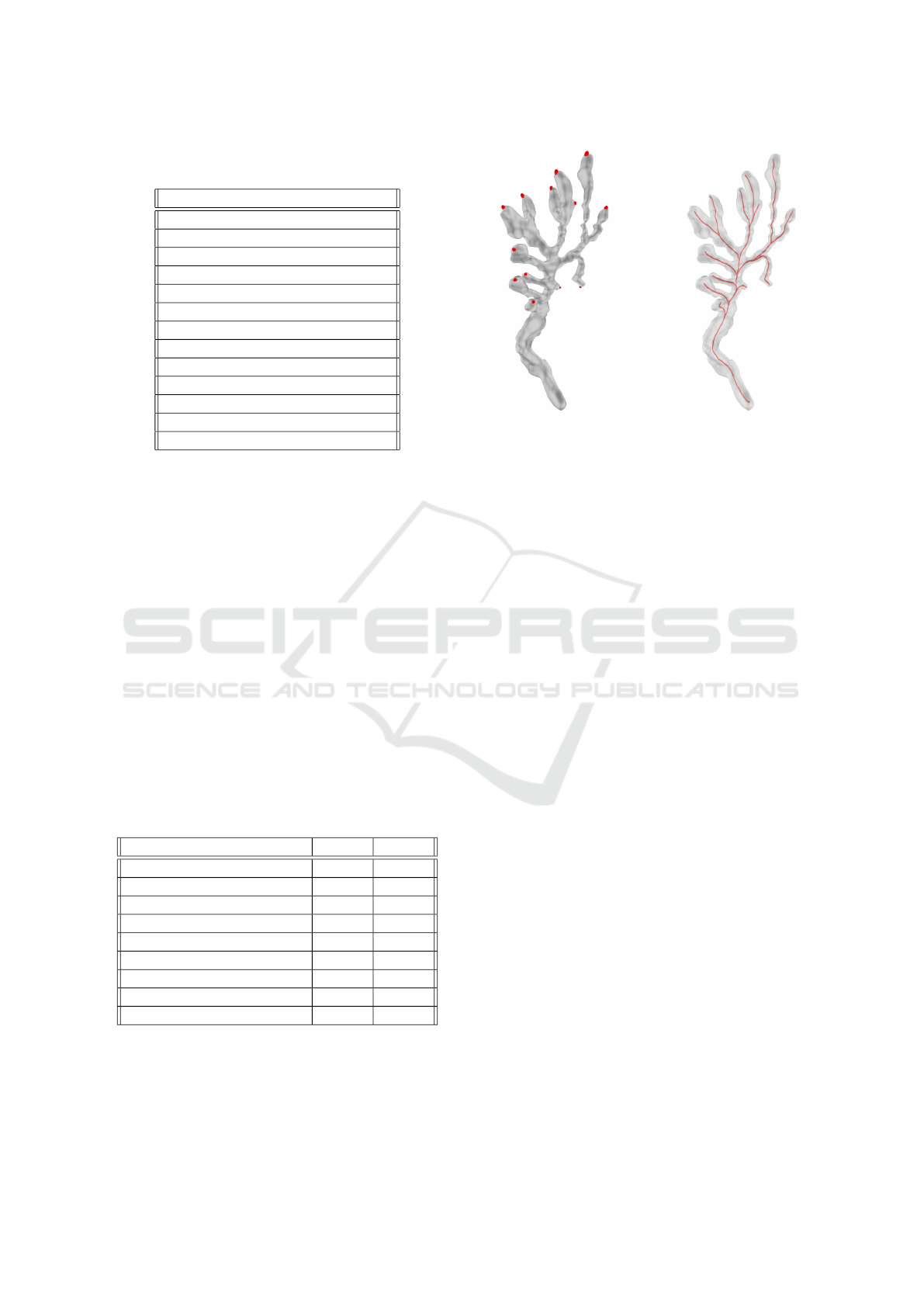
Table 1: A list of all available L-system parameters used in

algorithm 1.

Parameter name (units)

Segment radius (pixels)

Radial increment (pixels)

Bifurcation probability

Radial segments

Iterations

Iterations std.

Max. order

Segment branch length (pixels)

Segment branch length std. (pixels)

Upwards angle (degrees)

Upwards angle std. (degrees)

Bifurcation angle (degrees)

Bifurcation angle std. (degrees)

like structure, starting at the thicker bottom stem and

splitting to branches that vary in thickness, contains

few bifurcations and consequentially centerlines. For

this reason, it was used to test and verify the analysis

and the L-system parameter extraction methods dur-

ing the development of the web application. In this

section, the results of the ﬁnal analysis and L-system

generation from the extracted parameters are found.

For the preparation of the analysis, endpoints are

manually selected. In ﬁgure 2a, the selected endpoints

are shown in red. The stem at the bottom was picked as

the source point of the centerline structure. Endpoints

are chosen based on distinct branches and where they

approximately end in the mesh structure. Using this

method, 13 endpoints were selected. After selecting

the endpoints, the centerline in ﬁgure 2b was extracted.

Table 2: Attributes extracted from the analysis of the model

mesh in ﬁgure 2. Only the important attributes used for the

L-system generation are shown in this table. Thus, attributes

such as curvature, torsion and tortuosity are omitted.

Attribute name (units) Mean Std.

Branch length (pixels) 63.96 39.20

Point radius (pixels) 14.46 4.13

Centerline length (pixels) 582.56 123.60

Stem length (# iterations) 4.32

Bifurcations 11

Centerlines 13

Branches 24

Iterations 4.79 1.93

Bifurcation Angle (degrees) 62.81 19.45

The data collected from the analysis both from the

model and the centerline can be seen in table 2. A few

observations can be made from the table. Firstly, from

the 13 endpoints selected in ﬁgure 2a, 13 centerlines

(a) (b)

Figure 2: Model mesh of a lactiferous duct from newborn

mice. (a) shows the model mesh and the endpoint selections

used for the centerline creation (in red). (b) is the computed

centerline model illustrated inside of the original mesh.

have been created, meaning there are no incorrectly

analyzed centerlines. Secondly, the number of bifur-

cations does not entirely match the number of bifurca-

tions which can be found in ﬁgure 2b, because there

is also one trifurcation mistaken for a bifurcation. An-

other observation is that the total number of iterations,

which is in terms of how many mean branch lengths it

takes to build one mean centerline, is approximately

9 ± 2

. Finally, most of the varying data has a relatively

high standard deviation, but the branch length, exclud-

ing the stem length, has the highest standard deviation.

Figure 2b also displays this large variety in branch

lengths between bifurcations.

The parameters from table 2 were then used to ran-

domly generate L-systems. First, two L-systems were

selected from many similarly generated systems using

the given parameters, which can be found in ﬁgure

3. During this process, some L-systems were created

with colliding branches due to randomness of the algo-

rithm. These results were left out by using the prune

intersections option, as the original model does not

contain intersections. Furthermore, models with simi-

lar data extracted from the original mesh were selected

for the best representation. The three models were all

generated with ten iterations, because building each

segment needs at least two iterations. Additionally,

they vary in branch lengths, number of centerlines and

number of branches. The branch lengths range from

frequent short branches in ﬁgure 3a to frequent long

branches or a mixture in ﬁgure 3b.

Lastly, Figure 4 shows two L-systems with 13 cen-

terlines and varying iterations, iteration standard devi-

ation and no branch length standard deviation. These

Visualizing, Analyzing and Constructing L-System from Arborized 3D Model Using a Web Application

261

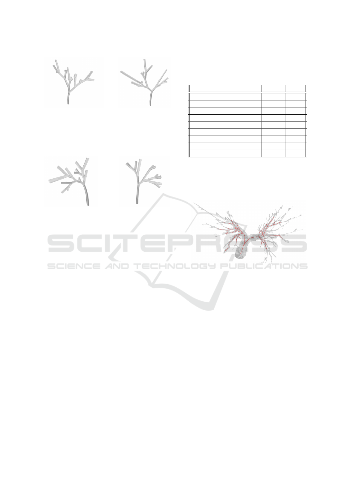
(a) (b)

Figure 3: A wide variety of randomly generated L-systems

based on the data from table 2 and with the number of iter-

ations set to 10. The upwards curve of the stem was set to

the standard value of 5 with a standard deviation of 2. (a) is

an L-system with 16 centerlines and 43 branches. (b) is an

L-system with 13 centerlines and 37 branches.

(a) (b)

Figure 4: Example of L-systems, based on the data from ta-

ble 2. The upwards curve of the stem was set to the standard

value of 5 with a standard deviation of 2. (a) is an L-system

with 38 branches, 10 iterations and no line std. (b) is an

L-system with 35 branches, 10 iterations, no iteration std.,

no branch length std. and 66% branch probability.

models were again selected from a pool of randomly

generated L-systems. Figure 4a shows a model where

the branch length standard deviation has been removed,

which removes extra long branches since all the branch

segment lengths are equal. The iteration standard devi-

ation has been reduced by one iteration. Consequently,

the variety in centerline lengths reduces. In Figure 4b,

the variety in centerline lengths has been completely

removed and the branch probability has been reduced

to retain a diverse amount of centerlines and bifurca-

tions. Due to the constant branch lengths, the overall

shape of the L-systems in ﬁgure 4 is more compact

compared to ﬁgure 3.

3.1.2 Artery

For the second case study, an artery 3D model was

used. The source of the model is derived from

www.sketchfab.com. This model has a more com-

plex tree-like structure starting at the much thicker bot-

tom stem and quickly decreasing in thickness. Some

branches are hardly connected to each other with

thin segments. Furthermore, the structure has a high

branching order and therefore contains many bifur-

cations and centerlines. Thus, it is used to test the

analysis and the L-system parameter extraction meth-

Table 3: Attributes extracted from the analysis of the artery

model. In the ﬁrst column, the attribute name and units are

shown. The second and third column show the mean and the

standard deviation if applicable.

Attribute name (units) Mean Std.

Branch length (pixels) 17.25 12.70

Point radius (pixels) 6.39 4.48

Centerline length (pixels) 150.04 20.86

Stem Length (# iterations) 2

Bifurcations 32

Centerlines 40

Branches 72

Iterations 6.82 1.20

Bifurcation angle (degrees) 44.40 37.68

ods on a more complex structure. For the analysis, 40

endpoints were chosen. Figure 5 shows the resulting

centerline model in the original mesh. We observed

that it contains many long branches compared to the

lactiferous duct model.

Figure 5: The original artery model with computed center-

line.

The data collected both from the model and the

centerline, can be found in table 3. Once again, some

observations can be made from this data. First, the

number of centerlines is inline with the number of end-

points. Second, the number of bifurcations is correct

since there are no trifurcations in this centerline model.

Next, the total number of iterations is approximately

9 ± 2

. Furthermore, most of the data has a relatively

high standard deviation just like in table 2, even though

there is more data available. Relatively, the bifurca-

tion angle standard deviation contains the highest and

the point radius the second highest standard deviation.

Contrary to the bifurcation angle standard deviation,

the relatively large branch length and point radius stan-

dard deviations can be observed by the alternation

between long and short branches together with the

thick inner branches close to the stem and thin outer

branches further away from the stem.

For the L-system generation from the attributes

acquired in table 3, We observed an abundance of col-

liding branches and centerlines, indicating that with

BIOIMAGING 2024 - 11th International Conference on Bioimaging

262

the given 14 iterations, too many branches were gen-

erated. Figure 6 shows L-systems without the branch

length standard deviation. In Figure 6a, the iteration

standard deviation was reduced, which is demonstrated

by the reduced number of outliers and radial develop-

ment. Figure 6b has no iteration and branch length

standard deviations but a branch probability. This lead

to equal centerline lengths and no more cut-off center-

lines compared to the systems generated before.

(a) (b)

Figure 6: Two randomly generated L-systems based on the

data from table 3. For all of the systems, the number of

iterations was set to 12. The upwards curve of the stem was

set to the standard value of 5 with a standard deviation of

2. (a) is an L-system with 40 centerlines, 85 branches, 2.39

segment radius, no branch length std. and one iteration std.

(b) is an L-system with 38 centerlines, 86 branches, 2.39

segment radius, no branch length std, no iteration std. and

76% branch probability.

Lastly, what can be observed from all the L-

systems which have been generated from the lactif-

erous duct and artery models, is the increased number

of branches compared to the number of centerlines.

The data in table 2 and 3 show that the original mod-

els require less branches to obtain the same number

of centerlines compared to what is produced by the

algorithm.

4 CONCLUSION AND

DISCUSSION

In this paper, we have focused on combining visual-

ization, analysis and L-system abstraction in a web-

environment. We generalized this functionality for

numerous arborized 3D biological structures. The vi-

sualizing capabilities were shown to be similar with

other visualization tools such as MeshLab (Cignoni

et al., 2008). On the other hand, the ability to visualize

3D models is limited by the user’s (web) resources,

which restricts the complexity of the models that can

be rendered.

Secondly, it has been illustrated that the function-

ality is sufﬁcient to perform proper statistical analysis

on branch-like structures and extract useful L-system

parameters. An important condition for the analysis

method is a sufﬁcient branch radius. However, no

speciﬁcation was given on which radii satisfy these

conditions. Another important condition, stated in the

VMTK documentation, requires the 3D model mesh

to be close-ended.

Next, L-system generation from extracted parame-

ters was shown. Changing the upwards and bifurcation

angle standard deviation did not seem to result in much

of a difference compared to the related work it was

derived from (Verbeek and Cao, 2020). In contrast,

the iteration and especially the branch length standard

deviation did have a signiﬁcant impact on the resulting

models. Removing the branch length standard devi-

ation made the overall shape look less chaotic and

more comparable to the centerline models in both ex-

amples. Depending on the type of abstraction, either

the original branch probability or the iteration standard

deviation can be utilized to add more variety to center-

line lengths. Thus, extracted parameters are viable to

generate L-systems, particularly branch lengths, radii,

angles and iteration standard deviation.

From these key results, we can conclude the

method described in this paper could be applied to

develop a web application that is in fact capable of

visualizing, analyzing and creating L-system abstrac-

tions of arborized 3D models. In addition, easy accessi-

bility and portability can provide workﬂow-improving

beneﬁts and the applied web development methods

contribute to extendibility.

For the future work, concerning visualization,

larger and more complex models could be supported

with server side rendering (Sawicki and Chaber, 2013)

or by rendering only speciﬁc sections of the 3D model.

The beneﬁt of this is that the client requires less re-

sources, but at the cost of more server resources and

the loss of real-time navigation and interaction. Be-

sides visualization, more (arborized) 3D model analy-

sis functionality and methods can be further extended.

This could include automated endpoint selection found

in Slicer (Kikinis et al., 2014), model pre-processing

methods for open-ended model analysis and error re-

duction (Izzo et al., 2018) or support for analysis of

multiple similar 3D models at once.

For L-system generation, additional statistical re-

search can be conducted on the distributions of the

parameters and how the data can be applied optimally,

particularly when dealing with relatively high standard

deviations. This also includes the right estimate of

iterations, which consistently failed during the testing

phase. Further experiments on L-system parameters

and resulting abstractions may give rise to models

which are more consistent and in accordance with the

requirements.

To conclude, VR features that are readily avail-

able within the A-Frame framework can be utilized.

Visualizing, Analyzing and Constructing L-System from Arborized 3D Model Using a Web Application

263

This includes VR interaction methods with the user

interface and new visualization capabilities (such as

a free-ﬂoating camera) that can change the way 3D

structures are analyzed and perceived.

REFERENCES

Balaji, S. and Murugaiyan, M. S. (2012). Waterfall vs. v-

model vs. agile: A comparative study on sdlc. Interna-

tional Journal of Information Technology and Business

Management, 2(1):26–30.

Boudon, F., Cokelaer, T., Pradal, C., and Godin, C. (2010).

L-py, an open l-systems framework in python. In De-

Jong, Theodore, Silva, D., and David, editors, 6th In-

ternational Workshop on Functional-Structural Plant

Models, pages 116–119, Davis, CA, United States.

Brewe, T. (2016). A l-system library using modern (es6)

javascript with focus on a concise syntax. http://https:

//github.com/nylki/lindenmayer.

C, R. (2010). Three.js 3d javascript library. http://github.

com/mrdoob/three.js.

Cao, L. (2014). Biological model representation and anal-

ysis. Phd thesis, Leiden Insitute of Advanced Com-

puter Science (LIACS) , Leiden University, Leiden, the

Netherlands. Available at https://hdl.handle.net/1887/

29754.

Cao, L. and Verbeek, F. J. (2012). Evaluation of algorithms

for point cloud surface reconstruction through the anal-

ysis of shape parameters. In Baskurt, A. M. and Sit-

nik, R., editors, Three-Dimensional Image Processing

(3DIP) and Applications II. SPIE.

Cao, L. and Verbeek, F. J. (2014). Nature inspired phenotype

analysis with 3d model representation optimization. In

Abraham, A., Kr

omer, P., and Sn

sel, V., editors, Inno-

vations in Bio-inspired Computing and Applications,

pages 165–174. Springer International Publishing.

Cignoni, P., Callieri, M., Corsini, M., Dellepiane, M., Ganov-

elli, F., and Ranzuglia, G. (2008). Meshlab: an open-

source mesh processing tool.

Cooper, D., Turinsky, A., Sensen, C., and Hallgr

ımsson,

B. (2003). Quantitative 3d analysis of the canal net-

work in cortical bone by micro-computed tomography.

The Anatomical Record Part B: The New Anatomist,

274B(1):169–179.

Foundation, B. (1998). Blender. org—home of the blender

project—free and open 3d creation software. http:

//blender.org.

Grinberg, M. (2018). Flask web development: developing

web applications with python. ” O’Reilly Media, Inc.”.

Gunicorn-Python, W. (2017). Http server for unix. URL:

http://gunicorn. org.

Izzo, R., Steinman, D., Manini, S., and Antiga, L. (2018).

The vascular modeling toolkit: A python library for

the analysis of tubular structures in medical images.

Journal of Open Source Software, 3:745.

Kikinis, R., Pieper, S. D., and Vosburgh, K. G. (2014). 3D

Slicer: A Platform for Subject-Speciﬁc Image Analysis,

Visualization, and Clinical Support, pages 277–289.

Springer New York, New York, NY.

Koch, N. and Kraus, A. (2002). The expressive power of

uml-based web engineering. In Second International

Workshop on Web-oriented Software Technology (IW-

WOST02), volume 16, pages 40–41. Citeseer.

Krasner, G. E., Pope, S. T., et al. (1988). A description of

the model-view-controller user interface paradigm in

the smalltalk-80 system. Journal of object oriented

programming, 1(3):26–49.

Mozilla (2015). A-frame, a web framework for building

virtual reality (vr) experiences. http://github.com/

aframevr/aframe.

of ISTI CNR, V. C. L. (2016). A javascript, client-side, mesh

processing tool. inspired by the well known meshlab.

https://github.com/cnr-isti-vclab/meshlabjs.

Prusinkiewicz, P. and Lindenmayer, A. (1990). The algo-

rithmic beauty of plants. Springer Science & Business

Media.

Reese, W. (2008). Nginx: the high-performance web server

and reverse proxy. Linux Journal, 2008(173):2.

Sawicki, B. and Chaber, B. (2013). Efﬁcient visualization

of 3d models by web browser. Computing, 95(1):661–

673.

van Ertbruggen, C., Hirsch, C., and Paiva, M. (2005).

Anatomically based three-dimensional model of air-

ways to simulate ﬂow and particle transport using com-

putational ﬂuid dynamics. Journal of Applied Physiol-

ogy, 98(3):970–980. PMID: 15501925.

Verbeek, F. J. and Cao, L. (2020). L-systems from 3d-

imaging of phenotypes of arborized structures. Funda-

menta Informaticae, 175(1-4):327–345.

BIOIMAGING 2024 - 11th International Conference on Bioimaging

264