Investigation of Workforce Dynamical Behaviour from a Phase Plane

Perspective

Timo Lahteenmaa-Swerdlyk and Franc¸ois-Alex Bourque

Centre for Operational Research and Analysis, Development Research and Defence Canada,

Keywords:

Differential Equation, Mentee, Mentor, Mentoring, Population Dynamics, Population Model.

Abstract:

The purpose of this work was to investigate the population dynamics of on-the-job training. The ratio of

mentees to mentors was considered, and its effect on overwhelming (saturating) the training system was anal-

ysed when undergoing a growth phase between two healthy states. This analysis was completed by analytically

solving a simpliﬁed continuous model of the problem with constant input parameters. The model was investi-

gated through a phase-plane interpretation, or the mentee versus mentor population as the system evolves. The

key input parameter of the analysis was the saturation limit: the ratio of mentees to mentors above which the

system becomes saturated. This value can be modiﬁed by adjusting various factors such as the quality, quan-

tity, and/or the delivery method of the training. Of special interest was the time for the system to evolve as the

saturation limit was varied. It was discovered that the system behaviour can fall into three categories based on

its value. If the saturation limit is very low, the system will remain saturated and never reach a steady state. If

the threshold is very high, the system will remain unsaturated (healthy) and reach steady state at inputted target

populations, albeit in a relatively slow timeframe. Finally, for a particular middle range of values, the system

will reach steady state at inputted target populations in an optimal time by crossing into and out of saturation.

Therefore, ﬁnding the optimal values for the input parameters will depend on a compromise between reaching

the target state quickly and not exceeding the target population levels, which will depend on the priorities of

the organization. Given that any occupation with on-the-job training could experience such effects during a

transition, understanding the dynamics of saturation is thus essential to design an efﬁcient training system.

1 INTRODUCTION

An important aspect of professional development is

on-the-job training. For military occupations such

as aircraft technicians (Bourque, 2019), this pro-

cess is formalized as a progression where appren-

tices (mentees) receive training under the supervision

of journeymen (mentors) before becoming mentors

themselves. Crucial to maintaining a healthy sys-

tem is the ratio of mentees to mentors: A low ratio

means that there are enough mentors to train all the

mentees present, and the system is in a healthy state.

However, too high a ratio causes the mentor popula-

tion to become taxed, potentially affecting their pri-

mary duties as well as stall the progression of the

mentees, as many are unable to be trained effectively.

While this scenario is usually avoided when the sys-

tem already possesses healthy population sizes, such

an event may occur when the system transitions be-

tween two healthy states. In practice, this satura-

tion effect may occur for any occupation undergoing a

transition with an on-the-job training component. For

example, in the case of a transition to a new aircraft,

the growth of the technician population able to main-

tain this new aircraft may be limited due to the lack of

journeymen able to supervise apprentices. Because of

this example and others, understanding the dynamics

of the saturation effect is important.

(Bastian and Hall, 2020) gives an excellent

overview of applied methods to perform military

workforce planning and modelling. Given the cou-

pled relationships present in on-the-job training sce-

narios and their associated complexities, discrete-

event simulations are the most common method of

analysing these systems (Novak et al., 2015; Zais and

Zhang, 2015; Henderson and Bryce, 2019). Another

common approach is to utilize industrial system dy-

namics (Forrester, 1965), which visualizes the con-

tinuous feedback loops, upwards ﬂow, and interac-

tion within these training structures (S

eguin, 2015).

Lahteenmaa-Swerdlyk, T. and Bourque, F.

Investigation of Workforce Dynamical Behaviour from a Phase Plane Perspective.

DOI: 10.5220/0012270900003639

Paper copyright by his Majesty the King in Right of Canada as represented by the Minister of National Defence

In Proceedings of the 13th International Conference on Operations Research and Enterprise Systems (ICORES 2024), pages 35-46

ISBN: 978-989-758-681-1; ISSN: 2184-4372

However, these structures are often difﬁcult to inves-

tigate due to their highly coupled nature. To allevi-

ate these issues, differential equations (Boileau, 2012;

Diener, 2018) and other statistical models (Bryce and

Henderson, 2020; Okazawa, 2020) are used to inves-

tigate simpliﬁed setups to verify the system dynam-

ics. However, this analysis is generally completed

with the populations already at a healthy state as this

greatly simpliﬁes the equations which are used (Di-

ener, 2018; Vincent and Okazawa, 2019). In prac-

tice, many key decisions must be made during transi-

tions between healthy states and these situations must

be analysed accordingly. To consider this, (Schaffel

et al., 2021) utilized a set of simpliﬁed differential

equations which is based on a predator-prey model

(Swift, 2002). This consists of a two-state model

which considers time-variable saturation effects on

the training rate of mentees as the mentor population

evolves. (Schaffel et al., 2021) investigated the sys-

tem using a benchmark scenario and applied it to a

Discrete Event Simulation. However, a deeper anal-

ysis of the governing equations are required to fully

understand its system dynamics and its application to

a realistic training scenario.

The aim of this paper is to analytically solve

and investigate this continuous two-state population

model by looking at its phase plane. The model fo-

cuses on an application to the training of aircraft tech-

nicians, which is its intended use. A benchmark sce-

nario is ﬁrst used as a backdrop to understand the sys-

tem behaviour as input parameters are adjusted, be-

fore investigating its analytical solutions. Special at-

tention is put into optimally reducing the time to reach

desired healthy populations. The remainder of this pa-

per is organized as follows. In Section 2, the system

of equations governing the upgrade process is intro-

duced, along with a benchmark scenario. Section 3

gives an overview of the system dynamics by plotting

numerical solutions of the benchmark scenario. Sec-

tion 4 then provides a more in-depth explanation of

the observations made in Section 3 by solving the in-

dividual training regimes and investigating their vari-

ous properties. The settling time is deﬁned and inves-

tigated in Section 5. Finally, in Section 6 two mathe-

matical proofs are completed to explain the behaviour

observed in Section 5.

2 MODEL FORMULATION

In this section, the system of equations which governs

the upgrading process of mentees to mentors is for-

mally introduced. In Section 2.1, the system of dif-

ferential equations governing the upgrading process

is stated. In Section 2.2, a benchmark scenario is in-

troduced to provide a base system for which we can

begin the analysis.

2.1 Model Introduction

From (Schaffel et al., 2021), the system of equations

to model the upgrade process is shown in Eqn. (1) and

Eqn. (2). The equations take the form of a modiﬁed

predator-prey model (Swift, 2002).

˙x = a −bmin(x,ry), (1)

˙y = bmin(x,ry) − cy, (2)

where x and y denote the mentee and mentor popula-

tions respectively, a is the intake rate of mentees into

the system; b is the healthy upgrade rate of mentees

to mentors, mentees requiring an average of 1/b time

units of mentoring before being upgraded; r is the sat-

uration limit, denoting the minimum number of men-

tors required to train one mentee; and c is the attrition

rate of mentors. To deﬁne the variable upgrade rate of

mentees, two possible regimes were considered:

1. The system is in the unsaturated training regime if

the ratio of mentees to mentors is less than the sat-

uration limit (x < ry), and there are enough men-

tors to train the entire pool of mentees in the sys-

tem. Therefore, the mentees upgraded at the nor-

mal rate (bx).

2. The system is in the saturated training regime if

the ratio of mentees to mentors is greater than

the saturation limit (x > ry), and there are no

longer enough mentors to train the entire pool of

mentees in the system. Therefore, the progression

of mentees to mentors is now limited to the number

of mentors, who can either spread their training out

equally among the pool of mentees, or focus their

training on a speciﬁc quantity of mentees up to the

value of the saturation limit. In either case, the rate

mentees upgrade to mentors is now bry.

In this system, it is assumed that the attrition rate (c)

may not be able to be readily changed, as mentors

generally leave the system due to retirements. How-

ever, the intake (a) and upgrade rates (b), as well

as the saturation limit (r), are controllable by adjust-

ing the quantity, quality, and delivery method of the

training, among other factors. Modifying these val-

ues may adjust the time required to transition between

two healthy states or add additional stress to the sys-

tem if the ratio of mentees to mentors becomes too

high. At the steady state, the rate of change of both

populations ( ˙x, ˙y) are equal to zero in the unsaturated

(healthy) regime, giving the relation:

a = bx

= cy

, (3)

ICORES 2024 - 13th International Conference on Operations Research and Enterprise Systems

where x

and y

denote the number of mentees and

mentors respectively in the target steady state. Since

the intake, upgrade, and attrition rates are tied to

the target population values, adjusting any of these

parameters will move the steady state values of the

mentee and mentor populations away from their in-

tended target populations. By ﬁxing the attrition rate,

the intake and upgrade rates are calculated to reach

the intended target populations.

This will leave the saturation limit as the sole in-

dependent variable, of which its effect on the system

will be the primary focus of this paper. Finally, we

are intrested in the case when the target mentor pop-

ulation is greater than the target mentee population

> x

). From Eqn. (3), this restriction results in

the upgrade rate being greater than the attrition rate

(b > c).

2.2 Benchmark Scenario

In the benchmark scenario, the mentee and mentor

populations will undergo a growth, transitioning from

an initial state (x

) to a target steady state (x

)

where the populations are doubled. The values chosen

are representative of an application to the training of

aircraft technicians. Speciﬁcally, the input parameters

are set to the following values:

) = (25,100)

) = (50,200)

c = 0.05

As discussed in Section 2.1, the intake (a) and up-

grade (b) rates are calculated to reach the target pop-

ulations:

a = cy

= 10

b =

= 0.2

From the deﬁned values, 10 mentees enter the system

on average each time unit, and each mentee requires

an average of 5 time units of training before upgrading

to a mentor when the system is healthy. A mentor then

stays in the system for an average of 20 time units

before exiting the pool.

3 SYSTEM DYNAMICS UNDER

THE BENCHMARK SCENARIO

To gain an initial understanding of the system dy-

namics, the system was numerically solved using

the fourth-order Runge-Kutta (RK-4) method. Phase

plane solutions of the benchmark scenario were plot-

ted as the saturation limit (r), the one independent

variable, was varied.

To break up the solutions to the system, we note

from Eqn. (1) and Eqn. (2) that the unsaturated region

is not dependent on r, so the changes in the system

behaviour will only occur in the saturated region. We

also note from Section 2.1 that the system will remain

saturated if the mentor population is decreasing (so

that x is always greater than ry). Therefore for a sys-

tem to exit saturation and reach steady state in the un-

saturated region, we require ˙y > 0. From inspection

of Eqn. (2), this occurs when br > c, or r > 0.25 in

the benchmark scenario.

Further analysis of the various solutions for the

benchmark scenario are completed in the subsequent

sections. In Section 3.1, system solutions that reach

the target populations are investigated (when r >

0.25). In Section 3.2, system solutions which do not

reach the target populations are investigated (when

r < 0.25). In Section 3.3, generalizations are made

of the system behaviour as r is varied.

3.1 System Solutions Which Reach the

Target Populations

An arbitrary value of r = 1/3 is chosen in Fig. 1

to showcase the relevant system dynamics, in which

there must be at least three times more mentors than

mentees to prevent the system from becoming satu-

rated. The solution trajectory and velocity vectors are

plotted, as well as the initial and target populations. A

dashed yellow line is added to visualize the saturation

limit, which is the ratio of mentees to mentors when

the system crosses into saturation. For reference, the

unsaturated region is present to the left of the line,

and the saturated region is present to the right. There

are two asymptotes in the unsaturated regime, a verti-

cal and diagonal asymptote, which are represented as

dashed-pink lines. From the plot, the solution begins

at the initial populations in the unsaturated region,

crosses into the saturated region, then curls, back into

the unsaturated region where it reaches steady state at

the target populations. The mentee population over-

shoots its target population, with its largest popula-

tion size occurring at the inﬂection point in the sat-

urated region. The system also exits the saturated

region below the diagonal asymptote in the unsatu-

rated region; with the mentor population approaching

its target population from below and does not contain

an overshoot.

As r is increased, the saturation limit line becomes

shallower, and the system spends less time in the satu-

rated region. Solutions of the benchmark scenario for

Investigation of Workforce Dynamical Behaviour from a Phase Plane Perspective

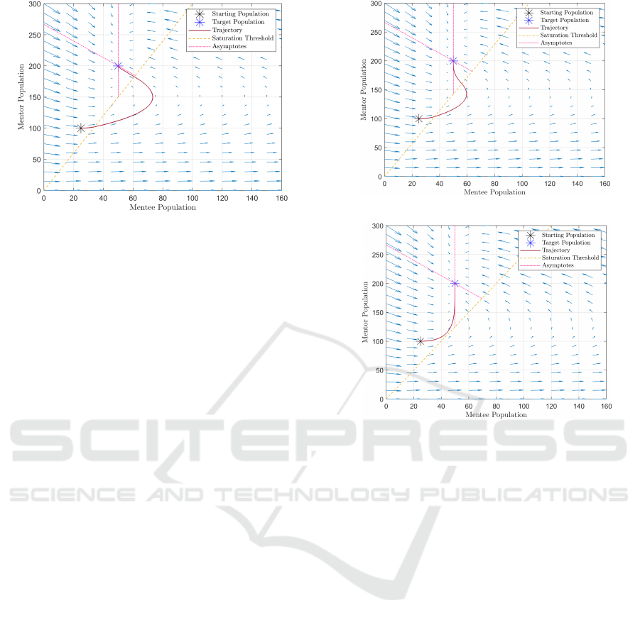
Figure 1: Phase plane of the benchmark scenario, with the

saturation limit (r) set to 1/3.

increased r values are shown in Fig. 2. In Fig. 2a, r is

set to 0.35, and in Fig. 2b, r is set to 0.4. Both solu-

tions reach the steady state at the target populations.

In Fig. 2a, the system has less of a mentee overshoot

than the plot of r = 1/3 shown in Fig. 1, with the

inﬂection point located at a smaller mentee popula-

tion. In Fig. 2b, we see that the saturation limit is high

enough that the system never becomes saturated. The

solution does not contain an inﬂection point as the

system is always unsaturated, with the largest mentee

and mentor populations located at their target popula-

tions. In addition, since the system remains in the un-

saturated region, the system no longer depends on the

value of the saturation limit, so the solution remains

unchanged if this value is further increased.

As r is decreased, the system spends more time in

the saturated region. Solutions of the benchmark sce-

nario for decreased saturation limit values is shown in

Fig. 3. In Fig. 3a, r is set to 0.3, and in Fig. 3b, r

is set to 0.28. As r is decreased, the inﬂection point

in the saturated region occurs at a larger mentee pop-

ulation, as both the mentor and mentee populations

experience greater overshoots from their target popu-

lations. In addition, the system takes longer to reach

steady state as more time is spent in the saturated re-

gion.

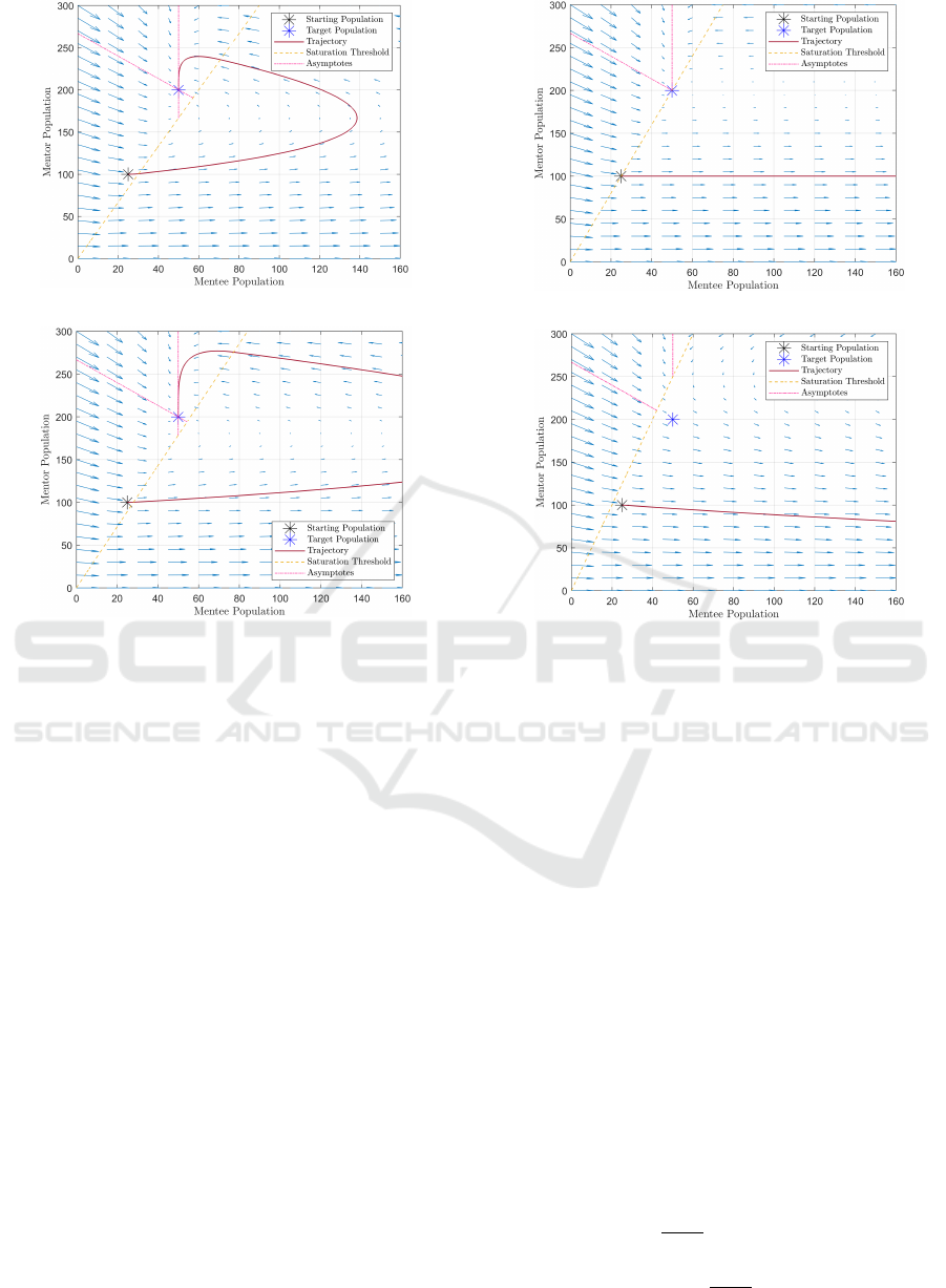
3.2 System Solutions Which Do not

Reach the Target Populations

Fig. 4 shows solutions for the benchmark scenario in

which the system does not reach the target popula-

tions. In Fig. 4a, r is set to 0.25, and in Fig. 4b, r is

set to 0.2. In Fig. 4a, the value of r is set such that

the upgrade rate is equal to the attrition rate (br = c).

As a result, the mentor population remains unchanged

from its starting value while the mentee population

increases to inﬁnity. In Fig. 4b, the value of r is set

(a) r = 0.35.

(b) r = 0.4.

Figure 2: Phase plane of the benchmark scenario, with the

saturation limit (r) set to 0.35 (top) and 0.4 (bottom).

such that the upgrade rate is less than the attrition rate

(br < c), in which the mentor population decreases to

zero while the mentee population increases to inﬁn-

ity. The target populations are also located in the sat-

urated region, so the system will never reach steady

state at the target populations regardless of the initial

populations.

3.3 Possible Behaviour for the System

From the phase plots in Section 3.1 and Section 3.2,

we can split up the possible behaviour into three sec-

tions depending on value of the saturation limit:

• When r ≤ c/b (r ≤ 0.25 for the benchmark sce-

nario), the system remains in the saturated region

and never reaches a steady state.

• When r is very high, the system reaches steady state

at the target populations but always remains in the

unsaturated regime.

• There exists a middle range of r values in which the

system reaches the steady state at the target popu-

lations, but crosses into the saturated region for a

period of time. This range is deﬁned on the low

ICORES 2024 - 13th International Conference on Operations Research and Enterprise Systems

(a) r = 0.3.

(b) r = 0.28.

Figure 3: Phase plane of benchmark scenario, with the sat-

uration limit (r) set to 0.3 (top) and 0.28 (bottom).

end by r > c/b (r > 0.25 for the benchmark sce-

nario), and on the high end by solving the unsatu-

rated region equations for the r value with the solu-

tion with one intersection point with the saturation

limit. For the benchmark scenario, this was found

to occur when r ≈ 0.3837, as the time in satura-

tion was zero. Above this r value, the system never

crosses into the saturated region.

We are most interested in the region of r values which

reach the steady state by crossing into the saturated re-

gion (0.25 < r < 0.3837 for the benchmark scenario),

as these solutions are dependent on more than one

system of equations. The subsequent analysis con-

tained in this paper will largely focus on this range of

r values.

4 ANALYTICAL SOLUTIONS

FOR AN ARBITRARY SYSTEM

From the plots of the benchmark scenario in Sec-

tion 3, several important observations were made: 1.)

The unsaturated region contains two asymptotes and

one steady state value, 2.) The saturated region has no

(a) r = 0.25.

(b) r = 0.2.

Figure 4: Phase plane of the benchmark scenario, with the

saturation limit (r) set to 0.25 (top) and 0.2 (bottom).

steady state value, and 3.) There was a range of r val-

ues in which the system reaches the target populations

by crossing into the saturated region. In this case, the

largest mentee population would occur at the system’s

inﬂection point in the saturated region. In this section

the individual regions are further investigated by solv-

ing their respective equations for an arbitrary system.

Section 4.1 and Section 4.2 provide an analysis of the

unsaturated and saturated regimes respectively.

4.1 Unsaturated Region

In the unsaturated region we have the following sys-

tem of equations:

˙x = a −bx, and (4)

˙y = bx −cy (5)

This region’s solution is shown in Eqn. (6) and

Eqn. (7).

x(t) = x

+ (x

− x

−bt

(6)

y(t) = y

c − b

− x

−bt



−

c − b

− y

)



−ct

(7)

Investigation of Workforce Dynamical Behaviour from a Phase Plane Perspective

The mentee (x) and mentor (y) populations decay to

the target populations of x

(a/b) and y

(a/c) respec-

tively as time increases, which are the target popula-

tions when the system reaches the steady state. The

system approaches the target populations regardless

of the initial population values (x

and y

To determine the asymptotes in the region, we can

ﬁnd the angle of the system around the target popula-

tion point in the phase plane, shown in Eqn. (8).

tan[θ(t)] =

y(t) − y

x(t) − x

c − b

−

c−b

− y

)

− x

)

(b−c)t

(8)

The asymptotes can be found by determining the

initial population values which result in a constant an-

gle (θ) for all time. From Eqn. (8), we see this is the

case when either the denominator is zero, or the time-

dependent exponential term is eliminated. Therefore,

we can ﬁnd the two asymptotes in the phase plane:

• A vertical asymptote when the initial and ﬁnal

mentee populations are the same (x = x

• A diagonal asymptote with the following equation:

y = y

c − b

(x − x

) (9)

The asymptote is at an angle centred around the tar-

get population point of θ = arctan(b/(c −b)).

From Eqn. (8), the angle of approach to the target

population point is ±π/2 as time increases to inﬁnity

since b > c. The only exception to this is if the tra-

jectory is located on the diagonal asymptote. Further-

more, a solution starting above the diagonal asymp-

tote will approach the target population point from

above at an angle of π/2, containing a mentor over-

shoot, while a solution starting below the diagonal

asymptote will approach the target population point

from below at an angle of −π/2. Using these asymp-

totes, we can ﬁnd the r value for the full solution

which exits the saturated region along the diagonal

asymptote. This value was numerically determined

using a bisection search and ﬁnding the system with

an angle of approach to the target populations which

is not ±π/2. For the benchmark scenario, this value

was found to be r ≈ 0.3317. This is analogous to a

critically-damped system, as this is the smallest possi-

ble saturation limit for the benchmark scenario which

prevents a mentor overshoot. The phase plane solu-

tion for this r value is shown in Fig. 5.

4.2 Saturated Region

In the saturated region we have the following system

of equations:

Figure 5: Phase plane of the benchmark scenario, with the

saturation limit (r) set to ≈ 0.3317.

˙x = a − bry, and (10)

˙y = −αy, (11)

where α ≡ c − br, the difference between the attri-

tion and upgrade rates in the saturated region. This

region’s solution is shown in Eqn. (12) and Eqn. (13).

x(t) =



−

bry



+ at +



bry



−αt

(12)

y(t) = y

−αt

(13)

The mentee equation contains a ramp term, so the

system does not have a steady state value. The be-

haviour of the saturated region is dependent on the

value of the saturation limit, the one independent vari-

able. If the attrition rate is greater than the upgrade

rate (c > br), then as time increases, the mentee pop-

ulation approaches inﬁnity and the mentor population

decays to zero. Likewise, if the upgrade rate is greater

than the attrition rate (c < br), then as time increases,

the mentee population approaches negative inﬁnity

while the mentor population approaches inﬁnity. Fi-

nally, if the two rates are the same (br = c), Eqn. (12)

and Eqn. (13) simplify to Eqn. (14) and Eqn. (15). As

time increases, the mentor population does not change

and the mentee population goes to either positive or

negative inﬁnity at a constant rate of a − bry

x(t) = x

+ (a − bry

)t (14)

y(t) = y

(15)

From Eqn. (12) and Eqn. (13), the inﬂection point of

a system in the saturated region can be calculated by

solving for when the derivative of the Eqn. (12) with

respect to x is zero, given in Eqn. (16) and Eqn. (17).

in f

, (16)

in f

= x

−



in f

+ ln



in f



− 1



, (17)

ICORES 2024 - 13th International Conference on Operations Research and Enterprise Systems

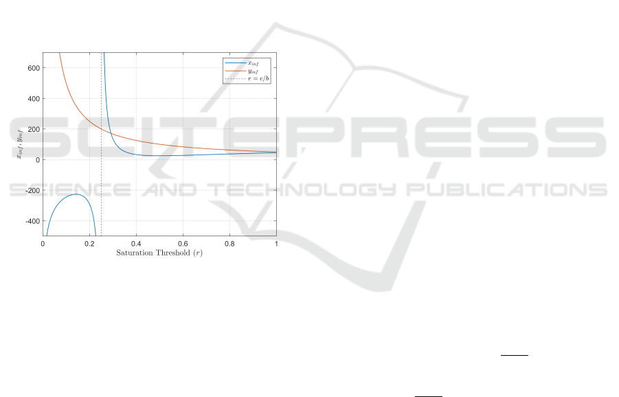
where x

in f

and y

in f

denote the mentee and mentor

populations respectively at the inﬂection point. The

inﬂection points for the benchmark scenario are plot-

ted in Fig. 6 for saturation limits between zero and

one. The mentee population at the inﬂection point

in f

) is shown in blue, and the mentor population at

the inﬂection point (y

in f

) is shown in orange. The

mentor population approaches inﬁnity at r = 0, and

decreases to zero as r is increased. The mentee pop-

ulation contains two asymptotes at r = 0 and r = c/b

(r = 0.25 for the benchmark scenario). For low val-

ues of r, the system has an inﬂection point at a mentee

population below zero and approaching negative in-

ﬁnity at the two asymptotes. For high values of r, the

mentee population approaches inﬁnity from the right

at r = c/b, then generally decreases as r is increased.

We can observe that the mentee and mentor popula-

tions at the inﬂection point increase as r is lowered to

r = c/b. This will put the system deeper into satu-

ration, putting additional stress on the mentors in the

system.

Figure 6: Mentee and mentor populations at the inﬂection

point for the benchmark scenario as r is varied.

5 TIME TO SETTLE AT A

THRESHOLD

As noted in Section 3.3, the system reaches the steady

state at the target populations in the unsaturated re-

gion. In this region, the mentee and mentor popula-

tions experience an exponential decay to their steady

state values, as noted in their respective equations,

Eqn. (6) and Eqn. (7) shown in Section 4.1. As a

result, the system approaches the target populations

asymptotically, with both populations requiring a time

of inﬁnity to reach their ﬁnal values. Therefore, to in-

vestigate the settling time of the system as the satura-

tion limit (r) is varied, a settling threshold is used as

a surrogate. In Section 5.1, a formal deﬁnition for the

settling threshold is given. In Section 5.2, the time

for the system to settle at a threshold is calculated.

Finally in Section 5.3, the time to settle at a given

threshold is analysed as the r is varied for the bench-

mark scenario.

5.1 Settling Threshold Deﬁnition

The settling threshold σ is deﬁned radially around

the target population point in the phase plane, with

the value of σ deﬁning the threshold radius. The

threshold equations in the phase plane are deﬁned

by Eqn. (18) and Eqn. (19), forming a circle centred

around the target population values.

x(σ) = σcos(θ) + x

, and (18)

y(σ) = σsin(θ) + y

, (19)

where θ ∈ [0,2π].

5.2 Time Components of a Solution

As noted in Section 3.3, there are three possible be-

haviours the system could follow: (1) If r is too

low, the system remains saturated and never reaches a

steady state. (2) If r is very high, the system reaches

steady state at the target populations, but remains un-

saturated for all time. (3) For an intermediate range of

r values, the system crosses into the saturated region

but still reaches steady state at the target populations.

For the second case, the settling time can be deter-

mined by solving the unsaturated equations given in

Section 4.1 for the time to reach the radial threshold

σ. This is completed in Eqn. (20) by ﬁnding the ra-

dius of the system around the target population point.

As the system is not dependent on r, Eqn. (20) can

be numerically solved for the time to reach a given

threshold value σ.

σ(t)

= [x(t) − x

]

+ [y(t) − y

]

− x

−bt



c − b

− x

−bt



−

c − b

− y

)



−ct



, (20)

where x

and y

are the starting populations. For the

third case, the process of ﬁnding the settling time is

stitched from three components:

• The time in the unsaturated region from the initial

population to the saturation limit. This can be deter-

mined by solving for the ﬁrst intersection point of

the unsaturated equations, Eqn. (6) and Eqn. (7) in

Section 4.1 with the saturation limit, x = ry. Com-

bining these three equations yields Eqn. (21). This

Investigation of Workforce Dynamical Behaviour from a Phase Plane Perspective

equation can be numerically solved for the time to

the saturation entry point.

0 = (ry

− x

) + (x

− x

)



c − b

− 1



−bt

+ r



−

c − b

− y

)



−ct

(21)

• The time in the saturated region between its two in-

tersection points with the saturation limit. This can

be determined similarly by utilizing the saturated

equations, Eqn. (12) and Eqn. (13) in Section 4.2,

for the system which starts at the saturation entry

point, solving for the second intersection point with

the saturation limit. The time in saturation is given

by Eqn. (22).

t =



− 1



−1

(α − b)e

(α−b)

(22)

where W

is the Lambert W Function, looking at its

k = −1 branch, α ≡ c − br, t is the time to the satu-

ration exit point, and x

is the mentee population at

the saturation entry point.

• The time in the unsaturated regime from the satu-

ration exit point at the saturation limit, to the given

threshold σ. This can be determined by inverting

Eqn. (20) for the time to reach σ, with x

and y

replaced as the saturation exit point coordinates.

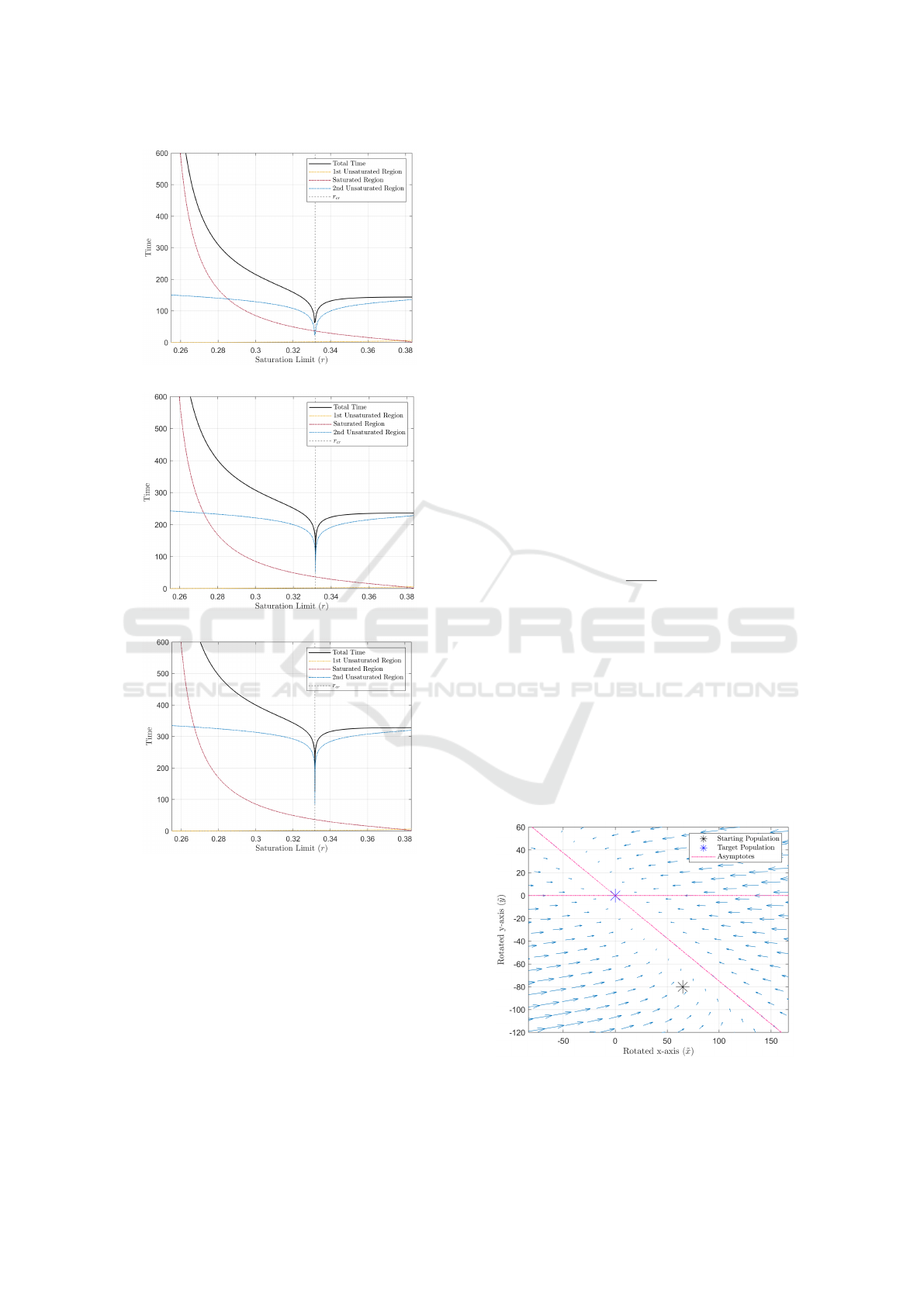
5.3 Time to Settling Threshold for the

Benchmark Scenario

Using the process deﬁned in Section 5.2, the settling

time was tabulated as r was varied for systems which

cross into saturation (0.25 < r < 0.3837 for the bench-

mark scenario). This is shown in Fig. 7 for an arbi-

trary threshold of σ = 1. The individual times the sys-

tem spends in each region are included, with the time

from the initial populations to saturation shown in yel-

low, the time spent in saturation shown in red, and the

time spent from saturation to the threshold σ shown

in blue. Finally, the r value for the system which exits

the saturated region along the diagonal asymptote in

the unsaturated region is shown as a dashed vertical

line labelled as r

, equal to r

≈ 0.3317 as noted in

Section 4.1. From the plot, it is observed that solu-

tions with low values of r take much longer to settle,

as more time is spent in saturation. As r increases,

the settling time approaches a speciﬁc value, which

is the time for the system if it were always unsatu-

rated. Finally, there exists a well which occurs solely

in the unsaturated region as the system approaches the

settling threshold. From the total settling time, the r

value for the minimum settling time is less than r

Therefore this solution overshoots the target mentor

population before decaying to the steady state.

Figure 7: Total settling time to threshold and breakdown of

time spent in each region for the benchmark scenario and

range of interested saturation limits. The settling threshold

is set to σ = 1.

The settling times for various saturation limits

were analysed as the threshold σ decreased to zero.

Shown in Fig. 8 are plots of the settling time for

decreased threshold values of σ = 10

−1

in Fig. 8a,

σ = 10

−3

in Fig. 8b, and σ = 10

−5

in Fig. 8c. From

the plots, the time to the saturation entry point and

in the saturated region remain unchanged, as they are

independent of the chosen threshold. In addition, the

total time to reach decreasing settling thresholds in-

creases for all values of r, given the exponential de-

cay to the target populations. However, the full width

at half maximum (FWHM) of the well decreases in

width, and the well increases in depth as the thresh-

old goes to zero. The r value for the minimum set-

tling time also drifts closer to r

as the threshold de-

creases. Therefore, the overshoot of the system with

the minimum settling time decreases as the threshold

goes to zero, approaching the system which exits the

saturated system along the diagonal asymptote in the

unsaturated region.

6 ANALYSIS OF AN ARBITRARY

SYSTEM NEAR STEADY STATE

To understand the behaviour observed in Section 5.3,

the interaction of the unsaturated region with the ra-

dial settling threshold is investigated by explaining

two mathematical proofs. In Section 6.1, the equa-

tions for the unsaturated regime are rotated to sim-

plify their form. Section 6.2 shows why the solution

with the minimum settling time at a non-zero thresh-

old is associated with a system overshooting the target

ICORES 2024 - 13th International Conference on Operations Research and Enterprise Systems

(a) σ = 10

−1

(b) σ = 10

−3

−5

Figure 8: Total settling time and breakdown of time spent in

each region for the benchmark scenario and range of inter-

ested saturation limits. The settling threshold is decreased

to σ = 10

−1

, 10

−3

, and 10

−5

mentor population. Section 6.3 demonstrates that as

the threshold is taken to zero, the solution along the

diagonal asymptote will eventually precede all other

non-diagonal solutions.

6.1 Simpliﬁcation of the Unsaturated

Region

To simplify the equations for the unsaturated region,

the system was re-centred around the target popula-

tion point and rotated such that the diagonal asymp-

tote is present along the new x-axis. The transformed

system is dubbed the ˜x(t) and ˜y(t) basis, with the ˜y(t)

basis vector perpendicular to the ˜x(t)-axis, the diago-

nal asymptote. This transformation is completed us-

ing a rotation matrix, with the angle of rotation (θ)

corresponding to the angle of the diagonal asymp-

tote in the unsaturated regime. The transformation

from the x(t) and y(t) basis to the ˜x(t) and ˜y(t) basis

is shown in Eqn. (23).



˜x(t)

˜y(t)





cos(θ) −sin(θ)

sin(θ) cos(θ)



x(t) − x

y(t) − y



, (23)

where θ = arctan [b/(b − c)], noted in Section 4.1.

The equations for the unsaturated regime in the

˜x(t) and ˜y(t) basis are given in Eqn. (24) and

Eqn. (25).

˜x(t) = ˜x

−bt

+ ˜y



b − c





−bt

− e

−ct



, (24)

˜y(t) = ˜y

−ct

, (25)

where ˜x

and ˜y

denote the starting coordinates in the

new basis, ˜x(0) and ˜y(0) respectively. A plot of the

phase plane in the new rotated basis for the bench-

mark scenario is shown in Fig. 9. Note that the diag-

onal asymptote in the original system now becomes

horizontal in the rotated system. In what follows,

the “diagonal asymptote” will refer to this horizon-

tal asymptote in the new rotated reference frame. In

addition, the “vertical asymptote” will refer to the di-

agonal asymptote which is present.

Figure 9: Phase plane of the unsaturated regime in the ro-

tated reference frame.

Investigation of Workforce Dynamical Behaviour from a Phase Plane Perspective

6.2 Settling Time at a Non-Zero

Threshold

We wish to understand why it was observed in Sec-

tion 5.3 that the solution with the minimum settling

time to a non-zero threshold corresponded to a sys-

tem with a mentor overshoot. As noted in Section 4.1,

these solutions are located above the diagonal asymp-

tote, or ˜y(t) > 0. In order for these solutions to reach

a threshold quicker, they must travel in the phase

plane at an increased velocity (i.e mentees are trained

faster). From Eqn. (25), the ˜y(t) component of a so-

lution is symmetrical across the diagonal asymptote

( ˜y = 0). Therefore, the difference in velocity must oc-

cur as a result of the movement in the ˜x direction. The

velocity of solutions in the ˜x direction can be calcu-

lated by taking the derivative of Eqn. (24) with respect

to time (t):

d ˜x(t)

= −b ˜x

−bt

+ ˜y



b − c





−ct

− be

−bt



(26)

The second term in Eqn. (22) has a component de-

pendent on its distance from the diagonal asymptote

( ˜y), which is not symmetric across the asymptote. We

can examine the time-dependent portion of this term,

labelled as function f :

f (t) = ce

−ct

− be

−bt

(27)

At a time of zero, the function is negative since c < b,

while it becomes positive over time since the ﬁrst term

decays at a slower rate than the second term. There-

fore, for positive ˜y

values, the velocity at small times

in the ˜x direction is negative but has a larger magni-

tude than the solutions below the diagonal asymptote.

This occurs since there are more mentors present at

larger ˜y

values, so mentees are trained at a quicker

rate. At large times, these overshooting solutions will

then slow down approaching the vertical asymptote as

the velocity magnitude is now smaller.

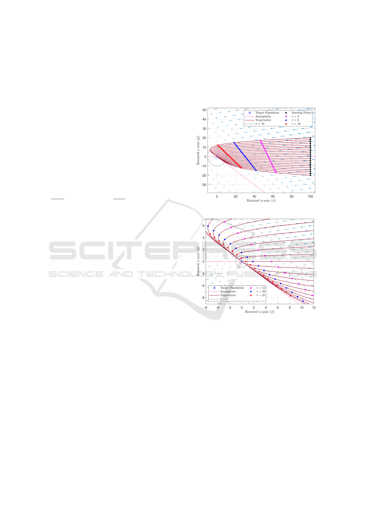
This behaviour can be observed in Fig. 10, in

which several solutions starting an arbitrary distance

of ˜x

= 100 away are plotted and sampled at various

times in Fig. 10a and Fig. 10b. At small times in

Fig. 10a, the solutions above the diagonal asymptote

are closer to the target population point, travelling at

an increased velocity relative to solutions below the

asymptote. As a result, several streamlines above the

diagonal asymptote reach the plotted settling thresh-

old of σ = 10. At large times in Fig. 10b, while all

solutions decay in velocity as they approach the tar-

get population point, the solutions above the diagonal

asymptote slow down and reverse direction. Only the

ﬁrst streamline above the diagonal reaches the smaller

settling threshold of σ = 1 in around 20 time units.

All other solutions have a mentor population which is

too high or low to reach the threshold. By extension,

as the settling threshold becomes smaller, the solu-

tion with the fastest time to the threshold must have

a smaller mentor overshoot, approaching the solution

along the diagonal asymptote.

(a) Sampled at time units of 3, 6, and 10. σ = 10.

(b) Sampled at time units of 15, 20, and 25. σ = 1.

Figure 10: Plot of several solutions starting x

′

= 100 away

from the target population point, sampled at various times.

An arbitrary settling threshold is also plotted.

6.3 Settling Time at a Threshold near

Zero

We wish to understand why it was observed in Sec-

tion 5.3 that the solution with the minimum settling

time to a threshold approached the solution along the

diagonal asymptote as the threshold was decreased to

zero. While this is a logical extension to the discus-

sion in Section 6.2, a mathematical proof for gener-

alized input parameters is given below. In the origi-

nal system, since the input parameters (a,b, c, r,x

)

can vary, a solution can approach the target popula-

ICORES 2024 - 13th International Conference on Operations Research and Enterprise Systems

tion point from anywhere in the phase plane. There-

fore, we need to show that given two systems in the

unsaturated regime: The ﬁrst starting along the diago-

nal asymptote an arbitrary distance away from the tar-

get population point, and the second which can start

anywhere else in the phase plane, the solution with

the minimum time to reach a threshold is the solution

along the asymptote, as the threshold nears zero. We

will deﬁne the system along the asymptote as System

1, and the system starting anywhere else in the phase

plane as System 2.

We note that if a system has the fastest time to

reach a threshold, then the all other systems are fur-

ther away from the target population at this time.

Therefore, we can show that the radius centred around

the target population from the ﬁrst system is always

less than the radius from the second system as time

approaches inﬁnity. The radii of the two systems rel-

ative to the target population can be calculated from

Eqn. (24) and Eqn. (25), shown in Eqn. (28) and

Eqn. (29). To simplify the equations, the substitu-

tions: τ ≡ e

−bt

, and φ ≡

b−c

are made. Eqn. (24)

and Eqn. (25) were used to ﬁnd the radii of the two

systems, shown in Eqn. (28) and Eqn. (29).

(τ)

= ( ˜x

τ)

, (28)

(τ)

= [ ˜x(τ)]

+ [ ˜y(τ)]

= ˜x

+ ˜y



2 ˜x

φτ

− 2 ˜x

φτ



+ ˜y

− 2φ



+ 1



(29)

where the starting distance from the target population

along the diagonal asymptote for System 1 is labelled

as ˜x

, and the starting coordinates for System 2 are la-

belled as ˜x

and ˜y

. Each of the starting coordinates

may be any real number other than zero, such that:

(1) The two systems are not separated by an inﬁnite

distance, (2) System 1 is not at the target population

point, and (3) Both two systems are not on the asymp-

tote. The difference in radii can found by subtracting

Eqn. (28) from Eqn. (29), shown in Eqn. (30).

(τ)

− σ

(τ)

= τ



˜x

− x

′2



+ ˜y



2 ˜x

φτ

− 2 ˜x

φτ



+ ˜y

− 2φ



+ 1



(30)

Since all systems reach the steady state at a time of

inﬁnity (τ = 0), taking the limit of Eqn. (30) as τ goes

to zero will yield a difference of zero. Therefore, it

must be shown that the difference in radii is positive

for small ﬁnite valuers of τ = ε, where ε is very close

to zero. From Eqn. (30), replacing τ with ε and writ-

ing out our required equality yields Eqn. (31).



˜x

− x

′2



+ ˜y



2 ˜x

φε

− 2 ˜x

φε



+ ˜y

− 2φ



+ 1



> 0

(31)

Eqn. (31) can be rearranged and divided through by

to yield Eqn. (32).

∴



˜x

− x

′2



+ 2 ˜x

˜y

φ + ˜y

−1



2 ˜x

˜y

φ + 2 ˜y



− ε

−1



+ 1



(32)

From Eqn. (32), the left-side can be any real, ﬁnite

value. For the right-side, ε

−1

is a negative exponen-

tial function and approaches inﬁnity as ε goes to zero.

Looking at the square-bracketed term, for a small but

ﬁnite value of ε, the second term will overpower the

ﬁrst term. Therefore, the right-side of the equation

will decrease exponentially to negative inﬁnity. As

a result, depending on the input starting coordinates,

two cases exist: (1) The right-side of the equation will

always be smaller than the left-side as ε is decreased,

or (2) The equation may not hold for larger values of

ε, but there is a value of ε in which the right-side will

decrease and be less than the left-side for all smaller,

but ﬁnite values of ε. In the ﬁrst case, System 1 will

always be ahead of System 2 for all times, while in

the second case, System 1 begins behind System 2

but overtakes it at a ﬁnite value of time. In either case,

System 1 will always end up closer to the target pop-

ulation point than System 2 as time increases, thereby

satisfying the equality.

Since the equality is satisﬁed, a system approach-

ing the steady state along the diagonal asymptote will

be the closest system to the target population for large

values of time, regardless of the starting coordinates

of any other arbitrary system. Therefore, a system

along the diagonal asymptote has the quickest time to

a threshold which is approaching zero.

7 CONCLUSION

In this paper, a continuous model was used to inves-

tigate the workforce population dynamics of on-the-

job training. Included in the model are the effects of

a high mentee to mentor ratio, when the mentors can

no longer train all the mentees present in the system.

When this occurs, the system is described by a sep-

arate, unhealthy regime. A key parameter of interest

was the saturation limit (r): the ratio of mentees to

mentors above which the system becomes unhealthy

(saturated). It was noted that to decrease the time for

the system to reach the target populations, r must be

set so that the system becomes saturated. This is to

orient the system to take advantage of the increased

Investigation of Workforce Dynamical Behaviour from a Phase Plane Perspective

velocity near the diagonal asymptote. It was proven

that the system with the minimum settling time at a

non-zero threshold contains a mentor overshoot and

will enter the saturated region; and as the threshold

is decreased to zero, the system with the minimum

settling time will approach the system which exits the

saturated region along the diagonal asymptote. This is

analogous to a critically damped system for the men-

tor population, in which the time to settle is optimally

reduced while having no overshoot of mentors.

In a realistic training scenario for aircraft techni-

cians, the time to train a required quota of new tech-

nicians can be reduced by allowing the system to be-

come saturated since this maximizes the total num-

ber of mentees trained at once. However, this will

require the system to become saturated and the pop-

ulations to overshoot. While overshooting the target

populations increases the time to a steady state, this

orients the populations to take advantage of the in-

creased training rate once the system exits saturation.

If there is a personnel cap which is imposed to prevent

a population overshoot, particularly for fully-trained

technicians (mentors), there are fewer technicians to

train the mentees and the system will take longer to

reach steady state. The diagonal asymptote represents

an equilibrium between maximizing the training rate

and keeping the populations close to their target val-

ues. While the training rate can be increased by hav-

ing more technicians, the drawback is that the num-

ber of technicians is further from the target value and

the total time is increased. Finally, the scenario cho-

sen corresponds to a growth phase where the popula-

tions are doubled. In a downsizing phase (e.g: pop-

ulations are halved), the system may never enter sat-

uration (depending on the initial ratio of mentees to

mentors) since there are fewer mentees to train. In

this case the system is more dependent on the attrition

rate, since the target values are reached once enough

mentors leave.

Moving forward with this model, time-dependent

input parameters can be investigated. The constant

values used for the parameters greatly restricted the

system dynamics. In a realistic model these param-

eters could vary as the system evolves to optimally

reduce the transient time and population overshoot,

while still reaching the target populations at their in-

tended values. For example, a solution with an op-

timally reduced time may hypothetically involve ad-

justing the input parameters over time to maximize

the training rate while orienting the trajectory to reach

the diagonal asymptote without becoming saturated.

REFERENCES

Bastian, N. D. and Hall, A. O. (2020). Military workforce

planning and manpower modeling. In Scala, N. M.

and Howard, J. P., editors, Handbook of Military and

Defense Operations Research. CRC Press, 1st edition.

Boileau, M. L. A. (2012). Workforce modelling tools used

by the canadian forces. pages 18–23.

Bourque, F.-A. (2019). Aircraft technician occupations:

A policy review. Reference Document DRDC-

RDDC-2019-D062, Defence Research and Develop-

ment Canada.

Bryce, R. and Henderson, J. (2020). Workforce popula-

tions: Empirical versus markovian dynamics. In 2020

Winter Simulation Conference (WSC), pages 1983–

1993.

Diener, R. (2018). A solvable model of hierarchical work-

forces employed by the canadian armed forces. Mili-

tary Operations Research, 23:47–57.

Forrester, J. (1965). Industrial Dynamics. System dynamics

series. Pegasus Communications.

Henderson, J. and Bryce, R. (2019). Veriﬁcation methodol-

ogy for discrete event simulation models of personnel

in the canadian armed forces. In 2019 Winter Simula-

tion Conference (WSC), pages 2479–2490.

Novak, A., Tracey, L., Nguyen, V., Johnstone, M., Le, V.,

and Creighton, D. (2015). Evaluation of tender solu-

tions for aviation training using discrete event simu-

lation and best performance criteria. In 2015 Winter

Simulation Conference (WSC), pages 2680–2691.

Okazawa, S. (2020). Methods for estimating incidence rates

and predicting incident numbers in military popula-

tions. In 2020 Winter Simulation Conference (WSC),

pages 1994–2005.

Schaffel, S., Bourque, F.-A., and Wesolkowski, S. (2021).

Modelling the mentee-mentor population dynamics:

Continuous and discrete approaches. In 2021 Winter

Simulation Conference (WSC), pages 1–10.

eguin, R. (2015). Parsim, a simulation model of the royal

canadian air force (rcaf) pilot occupation - an assess-

ment of the pilot occupation sustainability under high

student production and reduced ﬂying rates. In Pro-

ceedings of the 4th International Conference on Op-

eratinal Reserach and Enterprise Systems (ICORES).

Swift, R. J. (2002). A stochastic predator-prey model. In

Bulletin of the Irish Mathematical Society, number 48.

Irish Mathematical Society.

Vincent, E. and Okazawa, S. (2019). Determining equilib-

rium stafﬁng ﬂows in the canadian department of na-

tional defence public servant workforce. In 2019 In-

ternational Conference on Operations Research and

Enterprise Systems (ICORES), pages 205–212.

Zais, M. and Zhang, D. (2015). A markov chain model of

military personnel dynamics. International Journal of

Production Research, 54:1–23.

ICORES 2024 - 13th International Conference on Operations Research and Enterprise Systems