Dynamic Modeling and Effective Inventory Management for Uncertain

Perishable Supply Chains with non Synchronized Internal Dynamics

Beatrice Ietto

1,2 a

and Valentina Orsini

3 b

DIMA, UNIVPM, Ancona, Italy

Einstein Center Digital Future, Berlin, Germany

DII, UNIVPM, Ancona,Italy

Keywords:

Supply Chain Management, Supply Chain Modeling, Inventory Control, Perishable Goods, Robust MPC.

Abstract:

The problem we consider is to deﬁne an efﬁcient management strategy for a periodic-review production-

inventory system whose dynamics is characterized by various elements of complexity. These elements charac-

terize the vast majority of practical situations and consist of: 1) perishable goods with unknown deterioration

rate, 2) an uncertain future customer demand with oscillations that are not statistically modelable, 3) non-

synchronized operations of goods stocking and dispatching inside each review period. With reference to this

problem we deﬁne a general model of supply chain dynamics capturing the mentioned complex features and

encompassing, as particular cases, other models proposed in the literature. We also provide a coherent two cri-

teria based evaluation of the Bullwhip Effect (BE) and a Replenishment Policy (RP) resulting from a min-max

formulation of Model Predictive Control (MPC) approach. The RP maximizes the satisﬁed customer demand

and contains the BE within precise limits independent of the customer demand randomness.

1 INTRODUCTION

An effective control strategy of inventory level in

Supply Chains (SC) requires solving the challenging

problem of reconciling the following Control Speciﬁ-

cations (CSs): CS1) maximize the satisﬁed customer

demand (this is the primary goal), CS2) avoid over-

stocking, CS3) mitigate the Bullwhip Effect (BE).

The high conﬂictuality of these CSs calls for an op-

timality criterion. The widely acknowledged success

achieved by MPC in this regard is mainly due to the

ability to take into account the physical limitations

of the system, and to the receding horizon nature of

the control law that is continuously adapted according

to the incoming observations (Rossiter and Bishop,

2004). A thorough list of the very numerous MPC

based techniques dealing with different aspects of the

inventory problem in supply chain can be found in the

surveys (Sarimveis et al., 2008; Ivanov et al., 2018).

In this vast literature, only a few authors (see e.g.

(Gaggero and Tonelli, 2015; Taparia et al., 2020; Le-

jarza and Baldea, 2020; Hipolito et al., 2022)) con-

sidered the presence of deteriorating goods in the

https://orcid.org/0000-0001-5617-8228

https://orcid.org/0000-0003-4965-5262

inventory system, despite the acknowledged impor-

tance of the topic (Li et al., 2010; Chaudary et al.,

2018). Several alternatives to the MPC approach have

been proposed in (Ignaciuk, 2014; Ignaciuk, 2015;

Pan and Li, 2015; Le

sniewsky and Bartoszewicz,

2020; Cholodowicz and Orlowski, 2023) and refer-

ences therein.

All the previous contributions (MPC and non-

MPC) dealing with perishable goods assume an ex-

actly known deterioration rate. Unfortunately, this

simplistic assumption is not satisﬁed in the most

cases due to unstable and variable storage conditions

(Chaudary et al., 2018). Another important issue re-

gards the ”Internal Dynamics” (ID). With this syn-

tagm we deﬁne the sequence of OPerations (OP) in-

side each review period: OP1) updating the inven-

tory value; OP2) receiving goods from manufacturer;

OP3) dispatching goods to the customer; OP4) plac-

ing a replenishment order. A free planning of OP2 and

OP3 could be unrealizable due to several external fac-

tors independent of the SC manager. If the actual ID

is not properly taken into account in the design of the

RP, a serious SC performance degradation will occur,

especially in the case of highly perishable goods with

uncertain deterioration rate and a long review period.

A typical example is the food industry where the con-

Ietto, B. and Orsini, V.

Dynamic Modeling and Effective Inventory Management for Uncertain Perishable Supply Chains with non Synchronized Internal Dynamics.

DOI: 10.5220/0012269700003639

Paper published under CC license (CC BY-NC-ND 4.0)

In Proceedings of the 13th International Conference on Operations Research and Enterprise Systems (ICORES 2024), pages 25-34

ISBN: 978-989-758-681-1; ISSN: 2184-4372

sequent large waste and losses would result in a poor

economic sustainability.

To the best of our knowledge, what is still missing

about this issue is a general model of the inventory

level dynamics in the case of perishability under un-

certainty and a possibly unmanageable ID.

The main contribution of this paper is to ﬁll this

gap facing this topic at a formal level: here, we go

into the details of the ID, and propose a general model

of the dynamic SC encompassing other models pro-

posed in the literature, as particular cases. Taking

into account the possible non-synchronization of the

OPs allows us to obtain a model that more carefully

reﬂects the real dynamics of the SC and to deﬁne a

more effective RP conciliating CS1-CS3. From this

more general model we also derive a two-Evaluation

Criteria of the BE: EC1) smoothness of the RP, EC2)

”a priori” given bounds on the intervals over which

the RP takes values.

In accordance with EC1 we deﬁne a cost func-

tional adaptively penalizing excessive differences be-

tween two consecutive orders. As it concerns EC2,

we suitably compute the time varying constraints to

be imposed on the RP so as to guarantee the maxi-

mum amount of satisﬁed demand.

The actual computation of the RP is here set in

the same general theoretical framework used in (Ietto

and Orsini, 2022a; Ietto and Orsini, 2022b; Ietto and

Orsini, 2023a; Ietto and Orsini, 2023b) where the

OPs are assumed to be synchronized. The frame-

work consists in a min-max MPC whose solution is

parametrized using polynomial B-splines. The min-

max formulation of the MPC allows us to deal with

the uncertainties on the perishable rate and on the fu-

ture customer demand. The B-splines parametriza-

tion allows us: 1) to reformulate the min-max MPC

problem as a numerically simpler Constrained Robust

Least Squares (CRLS) problem; 2) to easily impose

hard constraints on the RP.

Compared to the latter references, we here provide

more theoretical and implementation insights : more

accurate description and prediction of the inventory

dynamics, a more accurate estimate of the constraints

on the control effort (i.e. the RP), deeper manage-

rial insights. E. g. in the case of manageable ID, the

man- ager can proﬁtably use the information from our

study for optimally scheduling the operations so as to

minimize the wastage due to deterioration.

The paper is organized in the following way.

Some mathematical preliminaries on B-splines and

RLS are recalled in Section 2 The system model is

described in Section 3. The min-max MPC problem

is stated in Section 4. In Section 5 the min-max MPC

problem is reformulated as a CRLS problem that can

be efﬁciently solved using second order cone pro-

gramming. Stability and feasibility are also discussed

(see Remark 6). Numerical results and concluding re-

marks are reported in Sections 6 and 7 respectively.

2 PRELIMINARIES

2.1 Polynomial B-Splines Functions

Polynomial B-splines functions are universal optimal

approximators of curves with complex shape. They

are deﬁned as a linear combination of B-splines basis

functions and control points, (De-Boor, 1978):

s(t) =

ℓ

∑

i=1

i,d

(t), t ∈ [

ℓ+d+1

] ⊆ R, (1)

where the c

’s are real numbers representing the con-

trol points of s(t), the integer d is the degree of the

B-spline, the (

)

ℓ+d+1

i=1

are the non decreasing knot

points and the B

i,d

(t) are the uniformly bounded B-

spline basis functions which can be computed by the

Cox-de Boor recursion formula. An equivalent repre-

sentation of s(t) in (1) is

s(t) = B

(t)c, t ∈ [

ℓ+d+1

] ⊆ R, (2)

where B

(t) = [B

1,d

(t),·· · ,B

ℓ,d

(t)] and

c = [c

,·· · ,c

ℓ

]

Convex hull property. Any value assumed by s(t),

∀t ∈ [

j+1

], j > d, lies in the convex hull of its d + 1

control points c

j−d

,·· · ,c

Smoothness property. Suppose that

i+1

= ··· =

i+m

i+m+1

, with 1 ≤ m ≤ d + 1 then the B-spline

function s(t) has continuous derivative up to order

d − m at knot

i+1

. This property implies that the

spline smoothness can be changed using multiple knot

points. It is common choice to set m = d + 1 multi-

ple knot points for the initial and the last knot points

and to evenly distribute the other ones. In this way (1)

assumes the ﬁrst and the ﬁnal control points as initial

and ﬁnal values.

2.2 The RLS Problem

Let A x ≈ b, be a set of linear equations, where A ∈

r×m

is the design matrix and b ∈ R

, r > m, is the

observations vector. Both A and b are subject to un-

known but bounded errors: ∥δA∥ ≤ β and ∥δb∥ ≤ ξ

(where the matrix norm is the spectral norm). The

RLS estimate x ∈ R

is the value of x solving the fol-

lowing min-max problem, (Lobo et al., 1998)

min

max

∥δA∥≤β, ∥δb∥≤ξ

∥(A + δA)x − (b + δb)∥ (3)

ICORES 2024 - 13th International Conference on Operations Research and Enterprise Systems

max

∥δA∥≤β,∥δb∥≤ξ

∥(A + δA)x − (b + δb)∥

= ∥Ax − b∥ + β∥x∥ + ξ (4)

Problem (3) is equivalent to minimize the following

sum of euclidean norms

min

∥Ax − b∥ + β∥x∥ + ξ (5)

The CRLS problem also requires that x satisﬁes the

following conditions

x ≤ x ≤ ¯x (6)

Remark 1. Note that the term ∥δb∥ in (3) only ap-

pears in (5) through its norm upper bound ξ, which is

independent of x. △

3 THE DYNAMIC UNCERTAIN

MODEL

retailer

manufacturer

issued order

u(k)

lead time

u(k-L)

actual customer demand

d(k)

fulfilled customer demand

h(k)

Figure 1: Single echelon SC model.

For ease of exposition and space limits we here con-

sider the simple SC model shown in Figure 1. Inside

each review period [kT (k + 1)T ), k ∈ Z

, the retailer

performs four OPs: OP1 determines its on hand stock

level; OP2 receives delivery from manufacturer; OP3

delivers the goods to meet demand; OP4 places a re-

plenishment order according to a suitably deﬁned RP.

We assume

• A1) OP1 takes place at the beginning of the re-

view period, OP2 and OP3 may not be simultane-

ous, OP2 is not subsequent to OP3, OP4 is exe-

cuted last;

• A2) the manufacturer fully satisﬁes each issued

non null replenishment order with a time delay

L = ℓT , ℓ ∈ Z

;

• A3) the goods arrive at the retailer new and dete-

riorate while kept in stock;

• A4) inside each review period of length T , the

uncertain perishability rate α

′

of the product is

deﬁned with respect to a sub-interval T

′

, with

T = nT

′

, n ∈ Z

, α

′

∈ [α

−

′

] ⊂ (0, 1), then

the corresponding decay factor over T

′

is ρ

′

1 − α

′

∈ [ρ

−

′

] ⊂ (0, 1).

MON

T’

(k+1)T

TUE

WED

THU FRI

SAT

SUN

T (a week) T’ (a day)

OP 1

OP 2

OP 3

y(k)

u(k-L)

h(k)

OP 4

u(k)

Figure 2: The operations performed by the retailer inside

each review period: OP1(Monday), OP2 (Wednesday), OP3

(Friday), OP4 (Saturday).

A clarifying example is shown in Figure 2 where we

suppose that T is a week and T

′

denotes a day of the

week (namely T = nT

′

with n = 7).

The customer demand is modeled according to the

following assumption

• A5) at any time instant k and limitedly to an M-

steps prediction horizon [k, k + M], the future cus-

tomer demand d(k + j), j = 0, ··· ,M, ﬂuctuates

within a compact set D

limited below and above

by two known boundary trajectories: d

−

(k + j)

and d

(k + j), j = 0,··· ,M. The set D contain-

ing the whole customer demand is given by the

consecutive contiguous overlapping of all the sets

,k ∈ Z

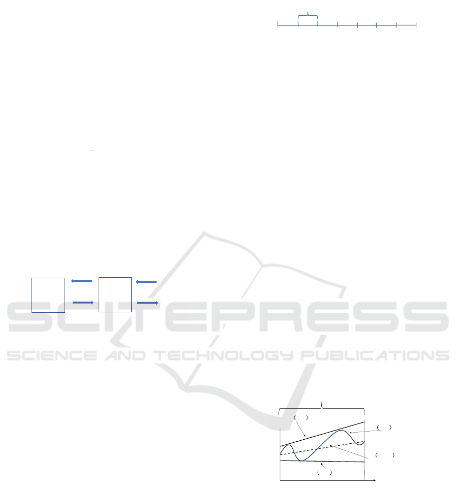
Figure 3 shows a typical example of a customer

demand d(k + j), j ≥ 0 over a ﬁxed D

. The

dashed line is the forecasted demand d(k + j|k),

j > 0. We assume it coincides with the central

trajectory

d(k + j) of D

. Hence, the actual future

values d(k + j), j > 0 can be expressed as

d(k + j) = d(k + j|k) + δd(k + j|k) (7)

where d(k + j|k) =

d(k + j) = (d

(k + j) +

−

(k + j))/2 is the predicted demand and δd(k +

j|k) is the corresponding estimation error.

𝑘 𝑘 + 𝑀

𝑑

𝑘 + 𝑗 , 𝑗 = 0, … 𝑀

𝑑 𝑘 + 𝑗|𝑘 , 𝑗 = 1, … , 𝑀

𝑑 𝑘 + 𝑗 , 𝑗 = 0, … , 𝑀

𝑑

𝑘 + 𝑗 , 𝑗 = 0, … , 𝑀

𝐷

Figure 3: An example of customer demand d(k + j), j =

0,··· ,M, over a ﬁxed D

. The dashed trajectory is the pre-

dicted demand d(k + j|k), j = 1,··· , M.

Remark 2. As |δd(k + j|k)| ≤ (d

(k + j) + d

−

(k +

j))/2, j = 1,· ·· , M, then δd(k + j|k) is the approx-

imation error sequence with minimum maximum ℓ

norm over each prediction interval. This is useful in

the CRLS formulation of the min-max MPC problem

because allows reducing the maximum norm of the

term that cannot be minimized with respect to x (i.e.

the term ξ in (5)). For more details see Remark 4 re-

ported in Section 5. △

Dynamic Modeling and Effective Inventory Management for Uncertain Perishable Supply Chains with non Synchronized Internal Dynamics

The above considerations imply that the stock

level dynamics is described by the following uncer-

tain equation

y(k + 1) = ρ

(ρ

y(k) + ρ

u(k − L) − h(k)) (8)

where:

- in accordance with A4), the quantities ρ

, ρ

and

in (8) are deﬁned as

△

= ρ

′

∈ [(ρ

−

′

)

,(ρ

′

)

] (9)

△

= ρ

′

∈ [(ρ

−

′

)

,(ρ

′

)

] (10)

△

= ρ

′

∈ [(ρ

−

′

)

,(ρ

′

)

] (11)

for some positive integers n

, n

and n

. For ex-

ample, with reference to Figure 2 we have: n

= 3,

= 4 and n

= 2.

- y(k) is the on hand stock level, i.e. the amount of

remaining undamaged goods available at the be-

ginning of the k review period; u(k − L) is the re-

plenishment order placed at time k − L and real-

ized at time k;

- h(k) is the fulﬁlled customer demand and by A1)

it is given by

h(k) = min(ρ

y(k) + ρ

u(k − L),d(k)) ∈ [0,d(k)]

(12)

where the quantity

y(k) + ρ

u(k − L) (13)

is the actual amount of goods available for sale

while the corresponding wasted goods is

(1 − ρ

)y(k) + (1 − ρ

)u(k − L)

△

= y

lost

(k) (14)

- the quantity

y(k) + ρ

u(k − L) − h(k)

△

= y

le f t

(k) (15)

is the amount of goods left in the stock just af-

ter OP1-OP3 have been performed. It follows

that inside each review period, the total amount

of wasted goods is

(1 − ρ

le f t

(k) + y

lost

(k)

△

= y

lost

(k) (16)

The model (8) generalizes the stock level balance

equations with nonperishable goods (ρ

= ρ

1) as well as those ones with synchronized OP2 and

OP3 (ρ

= 1) and also those ones with synchronized

OP1-OP3 at the beginning of the review period (ρ

= 1).

For future developments we now rewrite equation

(8) in a more convenient form where both ρ

′

and

d(k) are made explicit.

By (12) an equivalent expression of h(k) is

h(k) = d(k) − z(k) (17)

for some z(k) ∈ [0, d(k)] that represents the amount

of possibly unsatisﬁed demand.

Deﬁnitions (9)-(11) and condition (17) imply

y(k + 1) = ρ

′

(ρ

′

y(k) + ρ

′

u(k − L) − d(k) + z(k))

(18)

4 PROBLEM FORMULATION

The control problem we consider is to determine an

optimal RP matching the three antagonistic CSs de-

ﬁned in the introduction. Owing to the uncertainty

on the future demand and the deterioration rate, we

adopt a min-max MPC approach which requires to

repeatedly solve a min-max constrained optimiza-

tion problem over a future N steps control horizon

= [k k + N − 1] (for some N < M) and, accord-

ing to the receding horizon control, to only apply the

ﬁrst sample of the computed optimal control sequence

u(k + j|k), j = 0, 1,·· · ,N − 1.

At each ﬁxed k ∈ Z

and over the corresponding

control horizon H

, the min-max MPC is formally de-

ﬁned as follows:

min

u(k+ j|k)

max

′

∈[ρ

−

′

]

(19)

subject to: (7),(18), (20)

0 ≤ u

−

≤ u(k + j|k) ≤ u

< ∞ (21)

where

∑

i=1

(k + L + i|k)q

(k)e(k + L + i|k)

+λ(k)∆u

(k|k) (22)

e(k + L + i|k)

△

= d

(k + L + i) − y(k + L + i|k) (23)

∆u(k|k)

△

= u(k|k) − u(k − 1) (24)

By (7) and (18) we have

y(k + L + i|k) = ρ

)(L+i)

′

y(k)

L−1

∑

ℓ=0

)(L+i−ℓ)−n

′

u(k + ℓ − L)

i−1

∑

ℓ=0

)(i−ℓ)−n

′

u(k + ℓ|k)

−ρ

)(L+i)−n

′



d(k)− z(k)



−

L+i−1

∑

ℓ=1

)(L+i−ℓ)−n

′



d(k + ℓ) + δd(k + ℓ|k) − z(k + ℓ|k)



(25)

ICORES 2024 - 13th International Conference on Operations Research and Enterprise Systems

The following considerations are in order:

- by A5 and (23), it can be seen that M ≥ N + L;

- in the light of CS1 and CS2, requiring the on hand

stock level to track the maximum predicted cus-

tomer demand has a double beneﬁt: 1) the fulﬁll-

ment of CS1 without incurring the inconvenience

of the overstocking usually caused by a constant

reference level conservatively ﬁxed in advance; 2)

the implicit guarantee of a safety stock to reduce

the risk of lost sales and backorders, (Boulaksil,

2016).

- the hard constraints (21) need to guarantee the in-

ternal stability of the SC. Moreover, forcing the

control effort to ﬂuctuate within a predeﬁned am-

plitude range allows us to contain the BE. How to

compute u

−

and u

is explained in Section 4.1;

- the term λ(k)∆u

(k|k) has been introduced in or-

der to meet EC1: penalizing large deviations on

the control variables smoothes the control effort,

thus reducing its variability and the unavoidable

costs related to sharp order quantity changes;

- following (G.F. Franklin, 1990), the weights

(k), i = 1,·· · ,N, and λ(k), have been chosen

inversely proportional to the square of the interval

where the relative physical variables are allowed

to vary.

4.1 Computing the Bounds U

−

and U

The constraints u

−

and u

on u(k + j|k) have to be

properly determined on the basis of the two following

conﬂicting criteria: 1) the amplitude A

of the interval

−

]

△

= C

should be large enough to allow the RP

to follow demand ﬂuctuations, 2) too large A

should

be avoided in the light of EC2 (the second criterion

assessment of the BE).

Owing to the uncertainty on the future demand

d(k) and on the decay factor ρ

′

, we estimate u

−

and u

with reference to two possible, limit situa-

tions compatible with (18). Consider the following

scenario:

- the retailer is able to fully satisfy a customer de-

mand that, over each prediction horizon, is a con-

stant signal with value

∈ [d

−

]. This implies

z(k) = 0 in (18). The limits d

−

and d

are the min-

imum and maximum values respectively of the cus-

tomer demand over [k k + M].

- each control horizon H

is long enough to allow the

output (the on hand stock level), to practically attain

the steady-state value ˜y

under the forcing action of a

constant signal ˜u

The problem we now consider is: for any given con-

stant demand

∈ [d

−

] it is required to ﬁnd the

interval C

where the corresponding constant control

input ˜u

takes values, such that the resulting con-

stant steady state value ˜y

satisﬁes ˜y

≥

, ∀ρ

′

∈

[ρ

−

′

,ρ

′

Using classical z-transform methods and applying

the ﬁnal value theorem (Kuo, 2007) we have

˜y

′

(z−ρ

′

)



z=1

˜u

−

′

(z−ρ

′

)



z=1

(26)

If ρ

′

were exactly known, then, choosing ˜u

1−(ρ

′

)

+(ρ

′

)

(ρ

′

)

, equation (26) would readily

imply ˜y

. As ρ

′

is uncertain, the minimum

˜u

guaranteeing ˜y

≥

, ∀ρ

′

∈ [ρ

−

′

] is ˜u

1−(ρ

−

′

)

+(ρ

−

′

)

(ρ

−

′

)

Considering the two limit situations

= d

−

and

= d

we obtain

△

= [u

−

] =

′

−

] (27)

′

△

1−(ρ

−

′

)

+(ρ

−

′

)

(ρ

−

′

)

(28)

The amplitude A

of C

′

− d

−

) (29)

Conditions (27)-(29) give the ”a priori” estimate of

the BE corresponding to EC2. Condition (28) gener-

alizes to any possible ID the analogous ampliﬁcation

factor 1/ρ

−

estimated in (Ietto and Orsini, 2023b).

As 1/ρ

−

corresponds to 1/(ρ

−

′

)

, the two ampliﬁ-

cation factors coincide when OP1-OP4 are synchro-

nized at beginning of the review period. In fact, in

this case we would have n

= n, n

= n

= 0 and, by

(28):

′

= 1/(ρ

−

′

)

= 1/ρ

−

5 A MORE CONVENIENT

FORMULATION OF THE

MIN-MAX MPC

In this section we reformulate the min-max MPC as

a CRLS estimation problem. The purpose is to dras-

tically reduce the numerical complexity of the algo-

rithm solving the min-max MPC. For any ﬁxed k, the

functional J

, deﬁned in (19), is minimized assuming

that the control sequence u( j|k), j = k,··· ,k + N − 1,

is given by the sampled version (with sampling period

coinciding with the review period) of a B-spline func-

tion. Adapting the notation in (2) to specify that it is

relative to the k-th ﬁxed time instant we have

u( j|k)

△

= B

( j)c

, j ∈ [

ℓ+d+1

] (30)

Dynamic Modeling and Effective Inventory Management for Uncertain Perishable Supply Chains with non Synchronized Internal Dynamics

with

1. B

( j)

△

= [B

1,d

( j),·· · , B

ℓ,d

( j)]

2. c

△

= [c

k,1

,·· · ,c

k,ℓ

]

= ··· =

d+1

= k and

ℓ+1

= ··· =

ℓ+d+1

k + N − 1

4. the remaining ℓ −d − 1 knot points are evenly dis-

tributed over (k, k + N − 1)

Remark 3. Point 3 and the smoothness property of

B splines (recalled in Section 2.1) imply that the ﬁrst

sample u(k|k) of the B spline u( j|k) coincides with

the ﬁrst control point c

k,1

of the vector c

. △

The parameter vector c

deﬁning u( j|k), j =

k, ··· ,k + N − 1, is computed as the solution of the

CRLS estimation problem deﬁned beneath.

As ρ

′

∈ [ρ

−

′

], an equivalent representation of

′

+ δρ

′

△

= (ρ

−

′

+ ρ

′

)/2 (31)

where

′

is the nominal value and δρ

′

is the pertur-

bation with respect to

′

satisfying |δρ

′

| ≤ (ρ

′

−

′

)/2.

From (31) it follows that

′

= (

′

+ δρ

′

)

′

+ ∆ρ

′

(32)

where ∆ρ

′

△

= (

′

+ δρ

′

)

−

′

is the sum of all

terms containing δρ

′

in the explicit expression of

(

′

+ δρ

′

)

Exploiting (32), one has that the term

)(L+i)

′

y(k) of (25) can be rewritten as

)(L+i)

′

y(k) (33)

= (

)(L+i)

′

+ ∆ρ

′

,(n

)(L+i)

)y(k)

Analogously, the following terms of (25) can be

rewritten as

L−1

∑

ℓ=0

)(L+i−ℓ)−n

′

u(k + ℓ − L) (34)

L−1

∑

ℓ=0



)(L+i−ℓ)−n

′

+∆ρ

′

,(n

)(L+i−ℓ)−n



u(k + ℓ − L)

i−1

∑

ℓ=0

)(i−ℓ)−n

′

u(k + ℓ|k) (35)

i−1

∑

ℓ=0



)(i−ℓ)−n

′

+ ∆ρ

′

,(n

)(i−ℓ)−n



×B

(k + ℓ)c

)(L+i)−n

′



d(k)− z(k)



(36)



)(L+i)−n

′

+ ∆ρ

′

,(n

)(L+i)−n





d(k)− z(k)



L+i−1

∑

ℓ=1

)(L+i−ℓ)−n

′

d(k + ℓ) (37)

L+i−1

∑

ℓ=1



)(L+i−ℓ)−n

′

+ ∆ρ

′

,(n

)(L+i−ℓ)−n



d(k + ℓ)

L+i−1

∑

ℓ=1

)(L+i−ℓ)−n

′



δd(k + ℓ|k) − z(k + ℓ|k)



(38)

L+i−1

∑

ℓ=1



)(L+i−ℓ)−n

′

+ ∆ρ

′

,(n

)(L+i−ℓ)−n





δd(k + ℓ|k) − z(k + ℓ|k)



Equations (33)-(38) allow us: 1) to separate the terms

depending on the optimal control sequence u(k +

ℓ|k) = B

(k + ℓ)c

from the independent ones; 2) to

separate, in either groups of terms, the known quan-

tities from the unknown ones. Using (33)-(38), an

equivalent representation of the predicted tracking er-

ror given by (23), formally similar to that given in (3),

e(k + L + i|k) = (b

k,i

+ δb

k,i

) − (A

k,i

+ δA

k,i

(39)

where

k,i

= d

(k + L + i) −

)(L+i)

′

y(k) (40)

−

L−1

∑

ℓ=0

)(L+i−ℓ)−n

′

u(k + ℓ − L)

)(L+i)−n

′



d(k)− z(k)



L+i−1

∑

ℓ=1

)(L+i−ℓ)−n

′

d(k + ℓ)

δb

k,i

= −∆ρ

′

,(n

)(L+i)

y(k) (41)

−

L−1

∑

ℓ=0

∆ρ

′

,(n

)(L+i−ℓ)−n

u(k + ℓ − L)

+ ∆ρ

′

,(n

)(L+i)−n



d(k)− z(k)



L+i−1

∑

ℓ=1

∆ρ

′

,(n

)(L+i−ℓ)−n

d(k + ℓ)

L+i−1

∑

ℓ=1



)(L+i−ℓ)−n

′

+ ∆ρ

′

,(n

)(L+i−ℓ)−n



× (δd(k + ℓ|k) − z(k + ℓ|k))

ICORES 2024 - 13th International Conference on Operations Research and Enterprise Systems

k,i

i−1

∑

ℓ=0

)(i−ℓ)−n

′

(k + ℓ) (42)

δA

k,i

i−1

∑

ℓ=0

∆ρ

′

,(n

)(i−ℓ)−n

(k + ℓ) (43)

By Remark 3 also the term ∆u(k|k) = u(k|k) −

u(k − 1) = c

k,1

− u(k − 1) in (22) can be rewritten as

∆u(k|k) = (b

+ δb

) − (A

+ δA

(44)

where b

= −u(k − 1), δb

= 0, A

−



1 0 ··· 0



and δA

is a null row vector.

Deﬁning the following augmented column vectors

, b

, δb

of N + 1 elements







1/2

(k)e(k + L + 1|k)

1/2

(k)e(k + L + N|k)

1/2

(k)∆u(k|k)







, (45)







1/2

(k)b

k,1

1/2

(k)b

k,N

1/2

(k)b







δb







1/2

(k)δb

k,1

1/2

(k)δb

k,N

1/2

(k)δb







(46)

and the extended matrices A

and δA

of dimensions

((N + 1) × ℓ)







1/2

(k)A

k,1

1/2

(k)A

k,N

1/2

(k)A







δA







1/2

(k)δA

k,1

1/2

(k)δA

k,N

1/2

(k)δA







(47)

allow us to reformulate the min-max MPC (19)-(21)

as the following CRLS estimation problem:

min

max

∥δA

∥≤β

∥δb

∥≤ξ

∥(b

+ δb

) − (A

+ δA

∥

(48)

subject to u

−

≤ c

k,i

≤ u

, i = 1, · ·· ,ℓ. (49)

Constraints (49) derive from (30) and the convex hull

property of B splines.

By (3) (that is equivalent to (5)) and considering that

argmin

∑

∥g

(x)∥ ≡ arg min

(

∑

∥g

(x)∥)

it is seen that (48) deﬁne a problem of the kind (3).

Hence, according to Section 2.2, at any k, the solution

of the CRLS estimation problem (48)-(49) can be

determined solving

min

∥b

− A

∥ + β

∥c

∥ + ξ

(50)

where the components of c

must satisfy (49).

Remark 4. The maximum euclidean norm of the term

δb

given by (45) corresponds to the term ξ

of (50). It

is the analogous of the term ξ in (3). As ξ

is indepen-

dent of the control sequence u(k + j|k), j = 0 · ··N − 1

(i.e. the term x of (3)) its maximum norm can be min-

imized with respect to ∆ρ

′

and δd(k +ℓ|k) assuming

nominal ρ

′

and predicted customer demand given

by the respective central values

′

and

d(k + j), j =

1·· ·M. △

Remark 5. As for the numerical calculation of β

and ξ

, the following considerations hold: 1) as the

term ξ

of (50) is independent of c

, it cannot be min-

imized. Hence it can be removed from the objective

function; 2) only the upper bound β

on ∥δA

∥ needs

to be determined at each k. The way the B-spline basis

functions are deﬁned by the Cox de Boor formula im-

plies that B

(τ) = B

(τ+N), ∀τ ∈ H

, k ∈ Z

. Hence

by (43) and (47) one has that β

△

= β, ∀k = 0, 1,·· · and

moreover β is determined putting ρ

′

= ρ

′

. △

Remark 6. Feasibility and internal asymptotic sta-

bility of the proposed min-max MPC control strategy

are a direct consequence of the SC dynamics and of

our approach. Feasibility of (21) derives from: (30),

the consistency of (49) w.r.t. (48) and the convex

hull property of B-splines. The uniform boundedness

of all physical variables of the controlled SC derives

from: ρ

′

∈ (0,1), the assumed uniform boundedness

of d(k),k ∈ Z

and constraints (21). Both stability

and feasibility are independent of the length of the

prediction horizon.

6 ILLUSTRATIVE EXAMPLE

We consider a single echelon SC where the review

period is T = nT

′

= 2(weeks) with n = 14 and T

′

1(day). The model parameters are: L = 2 (lead time),

′

∈ [α

−

′

] = [0.05 0.1] (deterioration rate over

′

), ρ

′

∈ [ρ

−

′

] = [0.9 0.95] (decay factor over

′

) and y(0) = 0 (initial stock level).We suppose that

equation (18) is characterized by: n

= 8,n

= 6,n

4, so that ρ

= ρ

′

∈ [0.4305 0.6634], ρ

= ρ

′

∈

[0.5314 0.7351] and ρ

= ρ

′

∈ [0.6561 0.8145]. At

each k ∈ Z

, the min-max MPC is solved parametriz-

ing u( j|k) in (30) as a B-spline function of degree

d = 1 with ℓ = 3 control points.

This allowed us to verify that good results can

be obtained by simply imposing a C

continu-

ity and few control points. By (31) we have

′

= 0.925 and, according to Section 4, we

choose q

(k) =

(0.005·d

(k+L+i))

(i−1)

and λ(k) =

(0.005·u(k−1))

(weights in (22)). By Remark 5, we

Dynamic Modeling and Effective Inventory Management for Uncertain Perishable Supply Chains with non Synchronized Internal Dynamics

obtain that the parameter β

△

= β in (50) is given by

β = 0.6363. We also assumed an ”a priori” empir-

ical knowledge on the future customer demand lim-

ited to an M = 8 steps prediction horizon. Hence, the

length N of each control horizon H

has been chosen

as N = M − L = 6 .

Figure 4 shows the compact set D enclosing the

whole actual customer demand.

0 50 100 150 200 250 300

k review periods

the customer demand d(k)

Figure 4: The actual end customer demand d(k) (solid line).

The dashed lines represents the compact set D given by

the consecutive contiguous overlapping of all the ”a priori”

given sets D

’s.

The dynamic equation (18) has been implemented

assuming an actual ρ

′

= 0.9 and the simulation has

been stopped at time k = 280.

The generated RP is shown in ﬁgure 5. This ﬁg-

ure shows a control signal satisfying EC1 and EC2:

the RP has a smooth waveform and belongs to the

interval deﬁned by (27)- (28). The actual customer

demand d(k) and the fulﬁlled one h(k) are reported

in ﬁgure 6. This ﬁgure evidences the effectiveness of

the proposed RP: the customer demand is not satisﬁed

only for k ≤ L = 2, as a consequence of lead time and

null initial stock.

We have also carried out a second simulation to

show the effects of neglecting the available informa-

tion on the actual ID: we have calculated the RP under

the erroneous hypothesis that that all the OPs are syn-

chronized at the beginning of the review period. As

a consequence, the min-max MPC has been imple-

mented assuming n

= n = 14 and n

= n

= 0. Al-

though the amount of fulﬁlled customer demand is the

same, a serious performance degradation of the SC

is observed in terms of increased wasted and stocked

goods (see Table 1).

A performance degradation is also observed in

the EC2 measure of the BE: applying (28) we ob-

tain

′

= 3.7360 (actual ID) and a larger value

′

1/(ρ

−

′

)

= 4.3712 ( synchronized ID). Comparing

ﬁgures 5 and 7 shows that the interval containing the

RP is tighter in the min-max MPC strategy based on

the actual ID and CS1 is satisﬁed with a smaller con-

trol effort.

0 50 100 150 200 250

k review periods

100

120

140

160

180

The generated RP u(k)

Figure 5: The generated RP (solid line) and the boundaries

trajectories u

−

and u

(dashed lines) computed by (27)- (28)

with n

= 8 and n

= 4 and n

= 6.

0 50 100 150 200 250

k review periods

d(k) (solid line) h(k) (dashed line)

Figure 6: The actual customer demand d(k) (solid line) and

the fulﬁlled customer demand h(k) (dashed line).

0 50 100 150 200 250

k review periods

100

120

140

160

180

The generated RP u(k)

Figure 7: The generated RP (solid line) and the boundaries

trajectories u

−

and u

(dashed lines) computed by (27)- (28)

with n

= n = 14 and n

= n

= 0.

7 CONCLUSIONS

The rationale of our contribution is based on two con-

siderations: 1) the simplistic assumption of an exactly

known deterioration rate is never veriﬁed in practice,

2) the sequence of OPs inside each review period can

be imposed by external factors that can not be con-

trolled by the SC manager. To deal with these prob-

lems we introduced the notion of ID and deﬁned a

more realistic and general dynamic model encom-

passing many other SC models proposed in the litera-

ture. Endowing the min-max MPC with the informa-

ICORES 2024 - 13th International Conference on Operations Research and Enterprise Systems

Table 1: Quantitative performance evaluation.

wasted goods stocked goods

∑

280

k=0

lost

(k)

∑

280

k=0

y(k)

MPC (n

= 8, n

= 4, n

= 6) 14848 4999

MPC (n

= 14, n

= n

= 0) 17782 6318

tion carried by the actual ID yields a more effective

RP. In particular, the numerical simulations show a

signiﬁcant improvement in terms of reduced wasted

and stocked goods.

Our study also reveals the following managerial

insights with both academic and practical relevance:

• As stability and feasibility of the MPC control law

are guaranteed independently of the length of the

prediction horizon, the demand prediction prob-

lem is greatly facilitated;

• The worst-case approach provides the manager

with the security of an effective inventory control

despite the uncertainties;

• In the case of manageable IDs, our study pro-

vides the manager with the information necessary

to deﬁne the best organizational policy: equations

(14),(16) show that the waste of goods can be min-

imized synchronizing OP1, OP2 and OP3 at the

beginning of each review period.

REFERENCES

Boulaksil, Y. (2016). Safety stock placement in supply

chains with demand forecast updates. Operations Re-

search Perspectives, 3:27–31.

Chaudary, V., Kulshrestha, R., and Routroy, S. (2018). State

of the art literature review on inventory models for

perishable products. Journal of Advances in Manage-

ment Research, 1:306–346.

Cholodowicz, E. and Orlowski, P. (2023). Switching robust

neural network control of perishable inventory with

ﬁxed shelf life products under time-varying uncertain

demand. J. of Computational Science, 70.

De-Boor, C. (1978). A practical guide to splines. Springer

Verlag, New York, 2nd edition.

Gaggero, M. and Tonelli, F. (2015). Optimal control of dis-

tribution chains for perishable goods. IFAC Papers On

Line, 48:1049–1054.

G.F. Franklin, J.D. Powell, M. W. (1990). Digital Control of

Dynamic Systems. Addison-Wesley Publishing Com-

pany, N.Y, 2nd edition.

Hipolito, T., Nabais, J., Benitez, R., Botto, M., and Negen-

born, R. (2022). A centralised model predictive con-

trol framework for logistics management of coordi-

nated supply chain of perishable goods. International

Journal of Systems Science: Operation & Logistics,

9:1–21.

Ietto, B. and Orsini, V. (2022a). Effective inventory control

in supply chain with large uncertain decay factor. In

30th Mediterranean Conference on Control and Au-

tomation. IEEE.

Ietto, B. and Orsini, V. (2022b). Resilient robust model

predictive control of inventory systems for perish-

able good under uncertain forecast information. In

2022 International Conference on Cyber-physical So-

cial Intelligence (Best paper ﬁnalists award). IEEE.

Ietto, B. and Orsini, V. (2023a). Managing inventory level

and bullwhip effect in multi stage supply chains with

perishable goods: A new distributed model predic-

tive control approach. In 12th International Confer-

ence on Operations Research and Enterprise Systems.

SCITEPRESS.

Ietto, B. and Orsini, V. (2023b). Optimal control of inven-

tory level for perishable goods with uncertain decay

factor and uncertain forecast information: a new ro-

bust mpc approach. International Journal of Systems

Science: Operations & Logistics, 10:1–13.

Ignaciuk, P. (2014). Discrete inventory control in systems

with perishable goods- a time delay system perspec-

tive. IET Control Theory and Applications, 8:11–21.

Ignaciuk, P. (2015). Discrete time control of production-

inventory systems with deteriorating stock and unre-

liable supplies. IEEE Transactions on Systems Man

and Cybernetics, 45:338–348.

Ivanov, D., Sethi, S., Dolgui, A., and Sokolov, B. (2018).

A survey on control theory applications to operational

systems, supply chain management, and industry 4.0.

Annual Reviews in Control, 46:134–147.

Kuo, B. (2007). Digital Control Systems. Oxford University

Press, Oxford, 2nd edition.

Lejarza, F. and Baldea, M. (2020). Closed-loop real-time

supply chain management for perishable products.

IFAC PapersOnLine, 53:11458–14463.

sniewsky, P. and Bartoszewicz, A. (2020). Optimal

model reference sliding mode control of perishable in-

ventory systems. IEEE Trans. Autom. Science and En-

gineering, 17:1647–1656.

Li, R., Lan, H., and Mawhinney, J. (2010). A review on de-

teriorating inventory study. Journal of Service Science

and Management, 3:117–129.

Lobo, M., Vandenberghe, L., Boyd, S., and L

ebret, H.

(1998). Second-order cone programming. Linear Al-

gebra and its Applications, 284:193–218.

Pan, X. and Li, S. (2015). Optimal control of a stochastic-

inventory system under deteriorating items and envi-

ronments constraints. Int. Journal of Production Re-

search, 53:2937–2950.

Rossiter, J. and Bishop, R. (2004). Model Based Predictive

Dynamic Modeling and Effective Inventory Management for Uncertain Perishable Supply Chains with non Synchronized Internal Dynamics

Control. A Practical Approach. CRC PRESS, Boca

Raton, 1st edition.

Sarimveis, H., Patrinos, P., Tarantilis, C., and Kiranoudis,

C. (2008). Dynamic modeling and control of supply

chain system: A review. Computers and Operation

Research, 35:353–356.

Taparia, R., Janardhanan, S., and Gupta, R. (2020). Inven-

tory control for nonperishable and perishable goods

based on model predictive control. International

Journal of Systems Science: Operations & Logistics,

7:361–373.

ICORES 2024 - 13th International Conference on Operations Research and Enterprise Systems