Modeling iPSC-Derived Endothelial Cell Transition in Tumor

Angiogenesis Using Petri Nets

ela

Sterberov

, Andreea Dincu

, Stijn Oudshoorn

, Vincent van Duinen

and Lu Cao

1 a

Leiden Insisute of Advanced Computer Science, Leiden University, Leiden, The Netherlands

Leiden University Medical Center, Leiden, The Netherlands

Keywords:

Tumor Angiogenesis, Petri Nets, Endothelial Cell Transition, VEGF Gradient.

Abstract:

Tumor angiogenesis concerns the development of new blood vessels supplying the necessary nutrients for

the further development of existing tumor cells. The entire process is complex, involving the production and

consumption of chemicals, endothelial cell transitions as well as cell interactions, divisions, and migrations.

Microﬂuidic cell culture platform has been used to study angiogenesis of endothelial cells derived from human

induced pluripotent stem cells (iPSC-ECs) for a physiological relevant micro-environment. In this paper, we

elaborate on how to deﬁne a pipeline for simulating the transformation and process that an iPSC-derived

endothelial cell goes through in this biological scenario. We leverage the robustness and simplicity of Petri

nets for modeling the cell transformation and associated constraints. The environmental and spacial factors

are added using custom 2-dimensional grids. Although the pipeline does not capture the entire complexity of

tumor angiogenesis, we are able to capture the essence of endothelial cell transitions in tumor angiogenesis

using this conceptually simpliﬁed solution.

1 INTRODUCTION

Angiogenesis is the process of the development of

new blood vessels. Microvascular processes in angio-

genesis are found to play an important role in kidney

diseases, and are even described as ‘the base of the

iceberg’ for this category of disease (Querfeld et al.,

2020). The formation of blood vessels in tumors has

also been shown to inﬂuence metastasis and growth

rates (Folkman, 2002; Carmeliet and Jain, 2000; Toi

et al., 2002).

In recent years, human induced pluripotent stem

cells derived endothelial cells (iPSC-ECs) became in-

ﬂuential for disease modeling, drug discovery and

regenerative therapy. Microﬂuidic cell culture plat-

forms have been introduced to study angiogenesis of

iPSC-ECs in a physiological relevant cellular micro-

environment with controlled perfusion and gradients

(van Duinen et al., 2019). In this paper, we concen-

trated on modeling angiogenesis induced by VEGF

which is released by the hypoxic tumor cells in a mi-

croﬂuidic environment.

https://orcid.org/0000-0002-1847-068X

2 RELATED WORK

There are a number of mathematical and computa-

tional models developed to study different aspects of

angiogenesis (Peirce, 2008). A discrete mathemati-

cal model is developed for the dynamics of vascular

endothelial cells in angiogenic morphogenesis (Mat-

suya et al., 2016) It incorporates cell-mixing behavior

and temporal length generating behavior of the blood

vessel. A new mathematical model is designed to re-

produce the tumour-induced vascular networks under-

going stages of growth, regression and regrowth (Vi-

lanova et al., 2017). The model is able to capture cap-

illaries at full scale and the dynamics of vessel net-

works at long time scales. A mathematical formalism

is developed to simulate the early stages of angiogen-

esis based on a 3D in vitro model (Bookholt et al.,

2016). The model takes into account the dynamic in-

teraction and interchange of different phenotypes of

endothelial cells and several proteins playing a role in

the interaction. A hybrid model is developed to re-

alize silico experiments for tumor growth and angio-

genesis (Phillips et al., 2020). This model treats each

cell as an agent, incorporates phenotypic transitions

of each tumor and endothelial cell and allows VEGF

and nutrient ﬁelds to impact the dynamics.

Šterberová, A., Dincu, A., Oudshoorn, S., van Duinen, V. and Cao, L.

Modeling iPSC-Derived Endothelial Cell Transition in Tumor Angiogenesis Using Petri Nets.

DOI: 10.5220/0012268800003657

Paper published under CC license (CC BY-NC-ND 4.0)

In Proceedings of the 17th International Joint Conference on Biomedical Engineering Systems and Technologies (BIOSTEC 2024) - Volume 1, pages 337-346

ISBN: 978-989-758-688-0; ISSN: 2184-4305

337

These mathematical models are highly powerful

but they are not standardized enough for compari-

son. It also further hampers the reproducibility. We

are looking for a uniﬁed and versatile framework for

modeling biological systems. Petri nets is a graphi-

cal and mathematical formalism for the modeling and

analysis of concurrent, asynchronous, distributed sys-

tems (Chaouiya, 2007). It is shown to be a promising

mathematical tool to describe and study the relation-

ships and interactions between various parts of a bio-

logical systems e.g. metabolic pathways, organelles,

cells, and organisms (Carvalho et al., 2018; Valen-

tim et al., 2022; Liu et al., 2017). Furthermore, mul-

tiple variants of the initial formalism were created

(e.g. stochastic, timed, hybrid, coloured) to enable

analysing dynamical properties of complex processes,

from either a qualitative or a quantitative point of view

(Chaouiya et al., 2008).

In this paper, we utilized Petri nets to simulate the

transitions that iPSC-ECs undergo in the tumor angio-

genesis process in a microﬂuidic cell culture platform.

A complex pipeline is designed to model the diffusion

and consumption of the VEGF as well as the migra-

tion of the cells towards the VEGF gradient.

3 BIOLOGICAL DETAILS

A tumor induces the growth in quiescent arteries

when the tumor cells are depleted of nutrients, such

as oxygen. This growth induction is thus triggered in

hypoxic cells, causing them to excrete VEGF. VEGF

diffuses to the environment around the tumor and

causes the phalanx. Endothelial cells, that make up

the artery, start turning into tip cells by the inﬂuence

of VEGF. In addition, the VEGF acts as a chemoat-

tractant to tip cells. These cells inhibit neighboring

cells from turning into tip cells through notch sig-

nalling (Sainson and Harris, 2008). These neighbor-

ing cells turn into stalk cells instead. Stalk cells pro-

liferate and, meanwhile, follow the tip cell that is near

them. The tip cells inhibit the stalk cells from transi-

tioning back into phalanx cells within a certain dis-

tance. Therefore, the stalk cells can turn into pha-

lanx cells to stabilise the growing artery structure. In

Figure 1, an example of this stage in angiogenesis is

shown.

New physiologically relevant in vitro screening

was recently developed (van Duinen et al., 2019)

using iPSC-ECs in a microﬂuidic cell culture plat-

form, to model angiogenesis towards a VEGF gradi-

ent. This could be seen as a simpliﬁcation of vessel

growth near tumors, where the hypoxic tumor cells

are replaced by a VEGF gradient. In this paper, the

Figure 1: A visualization of the sprouting process. Red cells

are phalanx cells. Brown cells are tip cells and light brown

cells are stalk cells.

vessel formation is modeled in silico. The aim is to

create a model which includes transitions, movement,

differentiation and VEGF consumption of the cell. In

addition, the formation of a new blood vessel is also

induced. In this process, there are several cell types

with different roles. The methods that were used to

simulate these are further described in the following

sections.

4 METHOD

We developed a hybrid model that includes a central

Petri net and two grid matrices. The central Petri net

realizes the cell type transitions. The two grid matri-

ces deal in part with spatially connected features, such

as the cell positioning and movement, and the growth

vector (i.e. VEGF) concentrations.

4.1 Endothelial Cell Transitions Model

The endothelial cell type transitions are modeled us-

ing a timed hybrid Petri net in order to incorpo-

rate division/growing time, distance to the closest tip

cell and the VEGF concentration for each cell. The

scheme that we use is originally from (Phillips et al.,

2020) as illustrated in Figure 2. Because this scheme

is designed to mimic the movement of the tip cell ac-

cording to the gradient of VEGF which ﬁts our mi-

croﬂuidic environment the best. In addition, the pa-

per provides a detailed baseline parameters to work

with. It helps to bring biologically relevant proper-

ties to our model and makes our model more realistic.

The places in our model represent all the possible cell

types that an endothelial cell can adopt, namely: pha-

lanx cell P, stalk cell S, and tip cell T.

An additional place is added to represent the divi-

sion of stalk cells (SS). As the effect of this transition

is the separation of one cell into two smaller cells, two

different tokens have to be generated, adjacent to each

BIOINFORMATICS 2024 - 15th International Conference on Bioinformatics Models, Methods and Algorithms

338

Figure 2: Schematic illustration of endothelial cell tran-

sitions. d

tip

: the distance from the current cell to the

nearest tip cell. d

: Minimum distance from tip cell for

S → P transition. d

: Maximum distance from tip cell for

P → S transition. d

min

: Minimum distance from tip cell

for P → T transition. [VEGF]: VEGF concentration. α

VEGF threshold for P → T transition. τ: the amount of

time that a cell spends in a given place. τ

: a predeﬁned

time interval for a stalk cell to divide. τ

: growing time of

a stalk cell. τ

grow

: mandatory growing time.

other (positions (i, j) and (i − 1, j)). The introduction

of another token in the system has to be captured also

in the positioning grid, by ﬁlling an additional posi-

tion ((i − 1, j)). A stalk cell can divide after a prede-

ﬁned time interval (τ

), with each being half of its

original size and volume. For the newly divided stalk

cells to be considered again as integral stalk cells, they

have to go through a growing period to increase their

volume. This mandatory growing time is deﬁned as

a pre-set threshold, τ

grow

. Even if we have uniformed

the volume of the cell to a constant, the mechanisms

behind the growing phase are preserved.

The transitions in our Petri net correspond to pos-

sible changes in phenotype that a cell with a given

type can reach.

Each transition has to be conditioned in different

manners, as shown in Figure 2. The division of a stalk

cell (S → SS) and the transition of divided parts back

to an integral stalk cell (SS → S) are conditioned by

the passing of speciﬁc time intervals, τ

and τ

grow

re-

spectively. Additionally, the S → SS transition is con-

strained by the space available in the positioning grid.

Both the transition from phalanx cell P to stalk cell S

(P → S) and the reversed one (S → P) are conditioned

by the distance of a given cell to the nearest tip cell

tip

. For transitioning a phalanx cell P to a stalk cell

S, we have to ensure that the distance from a given

cell to a tip cell T is less than a pre-deﬁned threshold

, while when transitioning back from a stalk cell S

to a phalanx cell P, we need to have a tip cell T further

than a pre-deﬁned threshold d

. Finally, the transi-

tion from phalanx cell P to tip cell T (P → T ) is avail-

able only when there is no other tip cell in a certain

immediate vicinity (speciﬁed by d

min

) and the VEGF

at the location of the cell exceeds a certain value α

The distance to the nearest tip cell d

tip

is calculated

Table 1: Table with the ﬁxed parameters in our simulation.

Parameter Meaning Value

VEGF threshold for P → T

transition

0.1

γ Fixed consumption rate 10h

−1

Minimum distance from tip

cell for S → P transition

1.55

Maximum distance from tip

cell for P → S transition

1.55

min

Minimum distance from tip

cell for P → T transition

R Endothelial cell radius 1

S delay Stalk cell may divide after

this delay

SS delay Stalk cell growth time 3

based on the positioning grid, while the VEGF con-

centration is retrieved from the VEGF grid. The ﬁxed

thresholds used in the implementation can be found in

Table 1. These parameters are derived from baseline

set of model parameter values in (Phillips et al., 2020)

after unifying both tumor and endothelial cell radii to

1 so as to make our model biologically sound.

In order to prevent transitions in conﬂict situation

during simulation. The order of ﬁring the transitions

is set based on biological reasoning. We ﬁrst ﬁre the

S → SS transition, as there is no notion in our biologi-

cal framework that inhibits a cell from dividing when

the conditions for division are met. The same rea-

soning applies to the SS → S transition (which we set

as the second transition to be ﬁred) as when the cell

reaches the volume of a full stalk cell, it should be

immediately assigned to that phenotype. As the pos-

sible divisions of the stalk cells are already conducted,

the transition of the remaining stalk cells S to phalanx

cells P can be freely handled. The last two transitions

P → T and P → S are executed in this order. Even

if generally these two transitions are not concurrent,

in case such a situation might occur (based on the set

values of d

min

and d

), we would like to prioritize the

transition to a tip cell T when the VEGF condition is

met. By deﬁning a clear ordering, any concurrency

problems are mitigated.

The ﬁnal component of Petri nets that we need to

discuss is the token. In our model, a token represents

a speciﬁc cell, encapsulating various characteristics of

the deﬁned cell. The token’s internal representation is

{x, y, d

tip

, VEGF, τ}. x and y deﬁne the position of

the cell in the positioning matrix. d

tip

speciﬁes the

distance from the current cell to the nearest tip cell

(as computed using the positioning matrix). VEGF

indicates the VEGF concentration retrieved from the

VEGF grid at the cell position (x, y). τ stores the

amount of time that a cell spends in a given place.

Modeling iPSC-Derived Endothelial Cell Transition in Tumor Angiogenesis Using Petri Nets

339

Figure 3: Schematic illustration of the Petri net.

To create the Petri net, we used the Python

library SNAKES (Pommereau, 2015), which pro-

vides ﬂexibility in terms of modeling options or

extending the features. The source code is avail-

able at https://github.com/LuLIACS/angiogenesis-

modeling. The net scheme can be seen in Figure 3.

We can observe the places for each endothelial cell

phenotype (marked by circles). There are two types

of transition in the net. One type is a transition be-

tween different phenotypes. The other type of transi-

tion is a representation of time. The time is valid only

for two places, S and SS. In all transitions, t[i] refers to

speciﬁc information preserved in the token at position

4.2 Positioning and VEGF Grid

As previously introduced, there is a need in our model

to determine the distance between two cells. To de-

ﬁne a proper distance metric, one ﬁrst needs to set

the space in which the cells are placed. For conve-

nience, we chose to model this environment as a 2-

dimensional space, with the distance metric being the

Euclidean distance. In this manner, the integrity of

the biological concepts is preserved, and the extension

to the 3-dimensional space is fairly straightforward.

This kind of spatial representation can be interpreted

as a cross section of the original environment.

The grid was implemented as a 2-dimensional NumPy

(Harris et al., 2020) matrix, with conﬁgurable size

(H,W ). Each position in the matrix can hold a cell

or zero value when it is empty. This introduces the

limitation of all cells having the same volume, thus

the same growth factor consumption rate γ. The cell

is implemented as an object, initialized with the cell

type (phalanx, stalk, or tip). Subsequently, the func-

tions relevant to the cells are implemented on this ma-

trix, such as cell movement (changing positions of

cells), cell transition (changing cell types), calcula-

tion of the distance to the nearest tip cell, or division

of stalk cells. All of these functions are connected to

the Petri net and enabled for ﬁring. In order to simu-

late the formation of new blood vessels, the matrix is

initialized with all positions empty, except the bottom

row, ﬁlled with phalanx cells P. This row is meant

to depict a section of the micro-vessel culture in the

microﬂuidic well-plate.

The VEGF grid is similar to the positioning grid

and must match its shape. The VEGF grid was

also implemented as a 2-dimensional NumPy matrix,

which retains the concentration of VEGF present at

each position. The VEGF grid is initialized with only

the ﬁrst row holding non-zero concentrations. It sim-

ulates the existence of some tumor cells that emit the

VEGF signal. At each time step, a diffusion model is

applied. The diffusion model should deﬁne the way

in which the VEGF vector diffuses in our system.

We implemented two types of diffusion. The ﬁrst

one is regular. The part of the VEGF that is diffused

from the central position to a neighbor position with a

lower value of VEGF is given by diffusion factor f

which is set to 0.1 in our implementation. Therefore,

the value of VEGF in the center position and VEGF

in the neighborhood position can be given by

V EGF

center

= VEGF

center

− f

·V EGF

center

, (1)

V EGF

neighbor

= V EGF

neighbor

+ f

·V EGF

center

. (2)

But they are too regular and pleasant for a natural phe-

nomenon. Therefore, we implemented a second type

of diffusion with some level of randomness. In this

type of diffusion for each position in the grid, we ran-

domly decide which part of the VEGF amount should

diffuse in which direction (Hill, 2017). We again look

at each element in the VEGF matrix, and from this

center element, a random part of the VEGF amount is

diffused into each neighborhood position.

Additionally, the cells continuously consume part

of the VEGF according to their consumption rate γ.

In this manner, the VEGF grid has to be continuously

updated.

4.3 Cell Movement

Regarding the cell movement, we adopt a simpliﬁed

model. The movement is conditioned to happen only

upwards. After a cell transition to a tip cell, if the

tip cell is surrounded by stalk cells, the tip cell is al-

lowed to update its position. An additional type of

movement is the one when a stalk cell S divides. The

old cell has to be replaced by two new tokens which

represent the division into two smaller cells. In order

BIOINFORMATICS 2024 - 15th International Conference on Bioinformatics Models, Methods and Algorithms

340

to create space for the two tokens, all of the cells po-

sitioned in the previous rows are simply shifted one

row above, if there is space. In case there is no space,

the cell division does not take place, and the move-

ment does not happen. It particularly helps us to have

a natural end of the simulation, instead of allowing

cells to continuously multiply and push others outside

the grid. This design choice can be easily adapted as

needed.

4.4 Time Integration

As illustrated in Figure 2, certain transitions of the

cell type are time constrained. Moreover, the cell

movement and the diffusion of the VEGF have to be

discretized in order to be integrated into the model. A

natural way of doing this was to use time as our sam-

pling factor and update both the cell positions and the

VEGF concentrations once per time step. Thus, the

time factor is a necessary piece in all components of

our model. We introduced a custom way of model-

ing the time in order to better match the biological

scenario. In our approach, each cell (token) has an

internal individual timer τ which is reset to 0 when

the token enters a new place. This timer increases

for each cell independently until it reaches the time

constraint necessary for the connected transitions (i.e.

for the S → SS, the condition is τ > τ

). When the

condition is met, the transition can be ﬁred, and the

token has its timer reset. The timer increase can be

easily integrated into the Petri net using a loop transi-

tion so as to increment the τ variable inside the token

representation, until a set threshold (i.e. τ

). This

loop transition should be ﬁred at the start of each time

step. In this manner, the biological model is not com-

promised when implementing the time aspect, as any

number of cells are able to transition at the same time

step if needed.

5 EXPERIMENTS AND RESULTS

5.1 Diffusion Simulations

In the ﬁrst experiment, the two diffusion types are

compared with the same matrix initialization. The re-

sults of the simulations are shown in Figures 5 and 6

for normal and random diffusion, respectively.

In the ﬁrst simulation with the normal diffusion,

tip cells form on two sides of the grid at the same

time as shown in (a) of Figure 5. When these tip cells

are 1 square away from the top of the grid, enough

distance has accumulated and the two new tip cells in

the center form, both in time step 51.

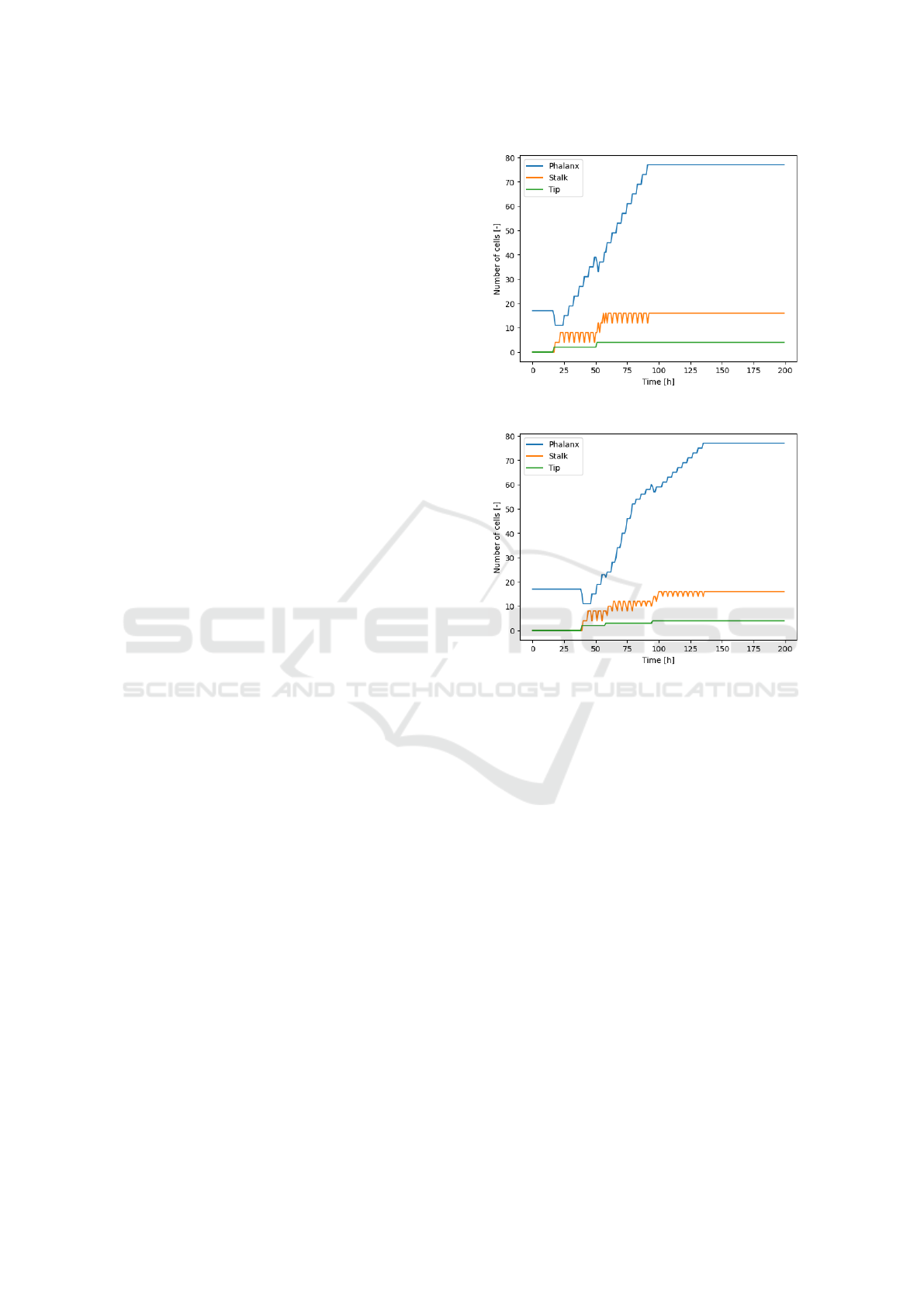
(a)

(b)

Figure 4: The number of cells shown per type for the normal

and random diffusion experiments.

The number of cells throughout the simulation is

depicted for each cell type in Figure 4(a). In this

graph the moments where the number of tip cells in-

creases, followed by the constant addition of phalanx

cells are visible.

The simulation with random diffusion, as shown

in Figure 6, also has two phalanx cells that transfer to

tip cells but on one side of the matrix at ﬁrst, which

happens 22 time steps later than with the normal dif-

fusion.

The count of the different cell types for this exper-

iment is shown in Figure 4(b). The third transition to

a tip cell happens on the left side at time step 58. The

two initial tip cells reach the top at 80, so the increase

in phalanx cells turns less steep. The fourth and ﬁ-

nal transition takes place as the third tip cell reaches

the top after which the increase in phalanx cells is

still less steep than during the growth of the ﬁrst two

branches.

The corresponding VEGF matrices for the nor-

mal and random diffusion are shown in Figures 7 and

Modeling iPSC-Derived Endothelial Cell Transition in Tumor Angiogenesis Using Petri Nets

341

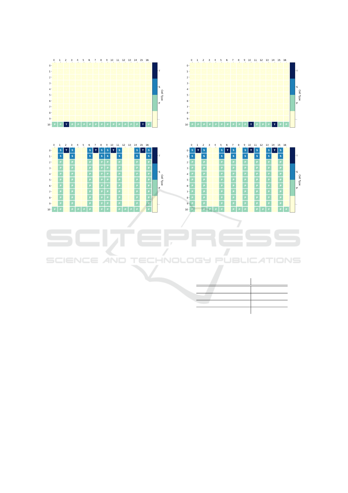
(a) Cell positioning - Iteration 17

(b) Cell positioning - Iteration 92

Figure 5: The cell matrix for the ﬁrst time step where tip

cells are formed (left) and where the ﬁnal movement of the

tip cells is seen (right). The time step is shown below the

ﬁgures.

8. The states on the left show the concentrations at

the time of the ﬁrst transition to a tip cell, while the

ones on the right are from the moment the last tip cell

reaches the top of the grid. A structured gradient is

observed and the matrix turns more symmetrical as

time passes in the simulation. After 115 steps the ma-

trix holds no VEGF anymore.

As random diffusion is not deterministic, differ-

ent states could be reached with the same initial state.

Note that the spreading patterns of the concentrations

do look similar at the same phase despite using dif-

ferent diffusion methods. The key difference is the

asymmetry that is observed, which follows from the

branching that started at one side. We quantiﬁed

the random diffusion, by running this experiment ten

times and averaging as shown in Table 2.

The average number of branches is observed to be

the same as in the normal diffusion simulation, which

suggests that random diffusion can be used to approx-

imate the normal diffusion.

5.2 VEGF Amount Experiments

In this set of experiments, we examined the inﬂuence

of the initial value of VEGF that is inserted into our

(a) Cell positioning - Iteration 39

(b) Cell positioning - Iteration 136

Figure 6: The cell matrix during the random diffusion ex-

periment when the ﬁrst tip cells form (left) and when the

ﬁnal movement is made by a tip cell (right). The number

below indicates the time step during the event.

Table 2: The average time step at which the described

events took place, and the average number of branches are

shown with their standard deviation.

Measurement µ ± σ

First tip cell 33.6 ± 6.7

First grown branch 74.6 ± 6.7

Number of branches 4.0 ± 0.7

Last grown branch 153.7 ± 23.7

environment. From the biological point of view, we

can assume that the environment closer to the tumor

contains a higher level of VEGF concentration than

the environment more distant from the tumor. There-

fore, a small amount of VEGF inserted into the model

may be seen as equivalent to the angiogenesis affected

by the tumor in the distance.

We performed these experiments with the same

initial settings; only the initial VEGF value differed.

We used the grid size 11 × 15 so that the cells have

enough space to grow. Parameter d

tip

was set to

10. And then, we performed 200 iterations with each

value of VEGF inserted into the grid. And all experi-

ments were conducted for both types of diffusion.

The results from the experiments are noted in

BIOINFORMATICS 2024 - 15th International Conference on Bioinformatics Models, Methods and Algorithms

342

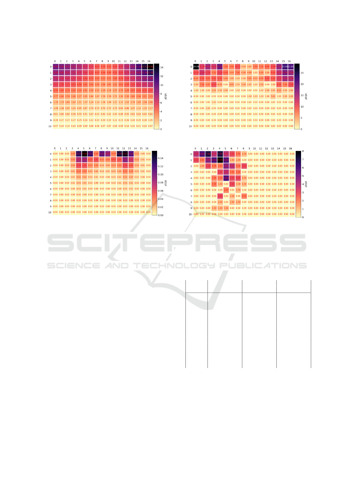
(a) VEGF grid - Iteration 17

(b) VEGF grid - Iteration 92

Figure 7: The VEGF concentrations for the normal dif-

fusion experiment, where the left frame shows the matrix

when the ﬁrst tip cell has formed and the right shows the

matrix when the last tip cell reaches the top of the matrix.

3, where we summed up the essential ﬁndings. 3

shows the results from the experiments with random

diffusion and regular diffusion. The ﬁrst column

(”VEGF”) shows the amount of initial VEGF. The

second column (”First transition”) indicates at which

iteration the ﬁrst transition of the cell phenotype oc-

curred. The third column (”First branch”) tells at

which iteration the ﬁrst branch was fully grown. The

last column (”Number of branches”) shows the num-

ber of branches that was grown in total. If the value is

noted by ’-’, the situation didn’t occur at all. Regard-

ing to regular diffusion, we observe that the minimum

amount of VEGF from the phalanx cell to the ﬁrst tip

cell is 300. Otherwise, the amount of VEGF, that dif-

fuses to the positions of the initial phalanx cells, is

trivial. Because it is consumed in each iteration until

there is no more VEGF left. We can also observe a

relation between the amount of VEGF and iteration

where the ﬁrst transition occurs. After exceeding the

limit amount necessary for the ﬁrst transition, the iter-

ations in which the ﬁrst transition took place decrease.

Furthermore, the iterations in which the ﬁrst branch

was fully grown decreased. On the other hand, with

random diffusion, we can not observe such relations.

The iterations in which the ﬁrst transition took place

(a) VEGF grid - Iteration 17

(b) VEGF grid - Iteration 92

Figure 8: The VEGF concentrations in the diffusion exper-

iments at the same time steps as in the normal diffusion in

Figure 7.

Table 3: Table of results from experiments with different

initial VEGF values, with random diffusion and regular dif-

fusion.

VEGF FT FB # branches

rand regu rand regu rand regu

50 27 - 68 - 3 -

100 30 - 72 - 4 -

150 36 - 78 - 3 -

200 53 - 94 - 3 -

300 43 19 84 60 3 1

400 32 15 74 56 3 3

500 26 13 68 54 4 3

600 33 12 73 54 3 3

700 27 11 68 52 4 3

800 37 10 78 52 5 3

900 35 10 76 52 3 4

1000 33 9 74 50 3 3

FT: First transition; FB: First branch; # branches:

number of branches

are around 27-53. But no pattern can be observed.

In addition, no pattern can be observed in a num-

ber of branches related to the amount of VEGF. For

example, the values are again random around 3-5.

With regular diffusion, it seems that the number of

branches is increasing with the amount of VEGF, but

it does not hold in all cases.

Modeling iPSC-Derived Endothelial Cell Transition in Tumor Angiogenesis Using Petri Nets

343

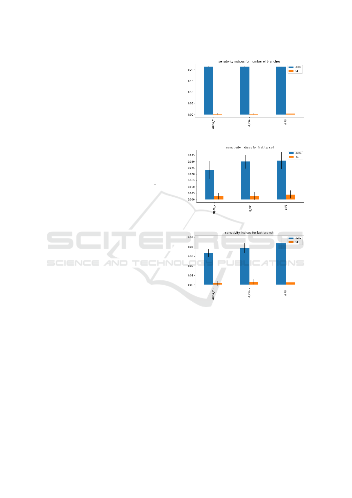
Table 4: Parameter range for sensitivity analysis.

Parameter range

[0, 3]

[0.5, 2.5]

min

[10, 15]

In general, we can observe that the number of

branches created is higher using random diffusion.

Moreover, the ﬁrst transition occurs sooner with ran-

dom diffusion. Therefore, we can conclude that using

random diffusion gives the model higher chances to

transition and grow new branches.

5.3 Sensitivity Analysis

Some of the parameters 1 that we used in our model

such as α

, γ, d

and d

are carefully estimated

in (Phillips et al., 2020). Some of them are ﬁne-

tuned to ﬁt our model scale such as d

min

, R, S delay

and ss delay. Nevertheless, we don’t know whether

iPSC-ECs behave the same during angiogenesis as

endothelial cells derived from adult mice or human.

Therefore, the parameters should be able to adjust and

we are interested to learn how sensitive is the model

to the choice of parameters. We selected three pa-

rameters, which have space to adjust in our model,

to conduct a sensitivity analysis. We set a range of

each parameter so that the cell transition is still hap-

pening within 200 iteration and the branch still grows

in a reasonable manner. A reasonable manner means

that there is only one tip cell on top of a branch while

growing and there is no single column branch that can

grow without a tip cell. With all the factors consid-

ered, we set the range for the three parameters as fol-

lowing:

We selected three features to be the output of the

model. They are the time step for the ﬁrst tip cell, the

time step for the last grown branch and the total num-

ber of branches. Delta Moment-Independent Measure

(Borgonovo, 2007) is used for sensitive analysis. It is

a global sensitive indicator which looks at the inﬂu-

ence of input uncertainty on the entire output distribu-

tion. In addition, the method returns ﬁrst-order sobol

indices which is a variance-based sensitivity (Sobol’

and Kucherenko, 2009). We set number of samples

equal to 1024 per parameter. The sensitive indices are

shown in Figure 9. We observed that, apart from the

sensitive indices for number of branches, the rest of

the indices are all very low and close to 0. That means

the parameters do not contribute much to the uncer-

tainty of the output of the model. That is probably

because our analysis model is relatively small with a

grid size 11 × 15. It does not give much variance in

the output features. In the future, a larger grid size

(a) sensitivity indices for number of branches

(b) sensitivity indices for ﬁrst tip cell

Figure 9: Results of sensitivity analysis.

should be considered for sensitivity analysis.

5.4 Scalability Experiment

The ﬁnal experiment that we conducted was designed

to test the scalability of our current implementation.

To attain this goal, we ran our simulation for a log-

arithmically increasing grid size, with the height and

weight varying in the interval [10, 10 000]. The cur-

rent implementation has an exponential increase of

running time, when the grid size is logarithmically in-

creased. Functions, such as the ones computing the

distance to the closest tip cell, executing the cell divi-

sion in the positioning grid and both VEGF diffusion

mechanisms, are computationally heavy. In the future

BIOINFORMATICS 2024 - 15th International Conference on Bioinformatics Models, Methods and Algorithms

344

work, we will look into the possibility of improving

these functions with the use of multi-processing or by

vectorizing the computations.

6 CONCLUSION

In this paper, we modeled the transformations that

iPSC-ECs undergo in the process of tumor angiogen-

esis in a microﬂuidics environment. The angiogen-

esis is guided by a gradient of VEGF. The model’s

behaviour was tested in various scenarios. Moreover,

sensitivity analysis and scalability analysis are con-

ducted to evaluate its performance.

The diffusion models were varied to ﬁnd the most

realistic one for model simulation. The diffusion

approximation through random particle movement

reached results that were very similar to those with

normal diffusion. It suggests that random diffusion

can be used to approximate the VEGF diffusion. The

non-symmetric formation of branches is also more

comparable to the chaotic branching seen in the in

vitro models. However, both approaches have their

drawbacks. Where the normal diffusion is too perfect

to be realistic, the random diffusion may result in too

large ‘jumps’ of particles to be realistic. In addition,

we found that the initial amount of VEGF does not in-

ﬂuence the speed of angiogenesis when using random

diffusion. But it is an essential parameter for regular

diffusion, where, with too low values of initial VEGF,

the angiogenesis does not start at all.

In this work, we used a rather simpliﬁed model

for cell movement, which only allows cells to move

upward. Side-way movement of tip cells should be

included in the future to make the model more real-

istic. Furthermore, the direction of motion should be

decided by the concentration of VEGF, while preserv-

ing contact with stalk cells.

Another limitation is the scale of the model with

a grid size 11x15. It is relatively small to indicate the

contribution of parameters to the uncertainty of the

output of the model. A larger grid size is preferred

for the sensitivity analysis. However, in scalability

analysis, we observed that the current implementation

has an exponential increase of running time when the

grid size grows logarithmically. In the future work,

functions with heavy computations should be further

investigated and the limitation on scalability of the

model should be solved using parallel computing.

REFERENCES

Bookholt, F. D., Monsuur, H. N., Gibbs, S., and Vermolen,

F. J. (2016). Mathematical modelling of angiogene-

sis using continuous cell-based models. Biomechanics

and Modeling in Mechanobiology, 15(6):1577–1600.

Borgonovo, E. (2007). A new uncertainty importance

measure. Reliability Engineering & System Safety,

92(6):771–784.

Carmeliet, P. and Jain, R. (2000). Carmeliet, p & jain, rk.

angiogenesis in cancer and other disease. nature, 407:

249-257. Nature, 407:249–57.

Carvalho, R. V., Verbeek, F. J., and Coelho, C. J. (2018).

Bio-modeling Using Petri Nets: A Computational Ap-

proach, pages 3–26. Springer International Publish-

ing, Cham.

Chaouiya, C. (2007). Petri net modelling of biological net-

works. Brieﬁngs in Bioinformatics, 8(4):210–219.

Chaouiya, C., Remy, E., and Thieffry, D. (2008). Petri net

modelling of biological regulatory networks. Journal

of Discrete Algorithms, 6(2):165–177. Selected pa-

pers from CompBioNets 2004.

Folkman, J. (2002). Role of angiogenesis in tumor growth

and metastasis. Seminars in Oncology, 29(6, Supple-

ment 16):15–18.

Harris, C. R., Millman, K. J., van der Walt, S. J., Gommers,

R., Virtanen, P., Cournapeau, D., Wieser, E., Taylor,

J., Berg, S., Smith, N. J., Kern, R., Picus, M., Hoyer,

S., van Kerkwijk, M. H., Brett, M., Haldane, A., del

ıo, J. F., Wiebe, M., Peterson, P., G

erard-Marchant,

P., Sheppard, K., Reddy, T., Weckesser, W., Abbasi,

H., Gohlke, C., and Oliphant, T. E. (2020). Array pro-

gramming with NumPy. Nature, 585(7825):357–362.

Hill, C. (2017). A very simple 2-d diffusion model.

Liu, F., Heiner, M., and Gilbert, D. (2017). Coloured Petri

nets for multilevel, multiscale and multidimensional

modelling of biological systems. Brieﬁngs in Bioin-

formatics, 20(3):877–886.

Matsuya, K., Yura, F., Mada, J., Kurihara, H., and Toki-

hiro, T. (2016). A discrete mathematical model for

angiogenesis. SIAM Journal on Applied Mathematics,

76(6):2243–2259.

Peirce, S. (2008). Computational and mathematical model-

ing of angiogenesis. Microcirculation (New York, N.Y.

: 1994), 15:739–51.

Phillips, C. M., Lima, E. A. B. F., Woodall, R. T., Brock, A.,

and Yankeelov, T. E. (2020). A hybrid model of tumor

growth and angiogenesis: In silico experiments. Plos

One, 15(4).

Pommereau, F. (2015). SNAKES: A ﬂexible high-level

petri nets library (tool paper). In Application and The-

ory of Petri Nets and Concurrency, pages 254–265.

Springer International Publishing.

Querfeld, U., Mak, R., and Pries, A. (2020). Microvascular

disease in chronic kidney disease: The base of the ice-

berg in cardiovascular comorbidity. Clinical Science,

134:1333–1356.

Sainson, R. and Harris, A. (2008). Regulation of angiogen-

esis by homotypic and heterotypic notch signalling in

Modeling iPSC-Derived Endothelial Cell Transition in Tumor Angiogenesis Using Petri Nets

345

endothelial cells and pericytes: From basic research to

potential therapies. Angiogenesis, 11:41–51.

Sobol’, I. and Kucherenko, S. (2009). Derivative based

global sensitivity measures and their link with global

sensitivity indices. Mathematics and Computers in

Simulation, 79(10):3009–3017.

Toi, M., Bando, H., Ogawa, T., Muta, M., Hornig, C., and

Weich, H. (2002). Signiﬁcance of vascular endothelial

growth factor (vegf)/soluble vegf receptor-1 relation-

ship in breast cancer. International Journal of Cancer

- INT J CANCER, 98:14–18.

Valentim, R. A. M., Caldeira-Silva, G. J. P., da Silva, R. D.,

Albuquerque, G. A., de Andrade, I. G. M., Sales-

Moioli, A. I. L., Pinto, T. K. d. B., Miranda, A. E.,

Galv

ao-Lima, L. J., Cruz, A. S., Barros, D. M. S., and

Rodrigues, A. G. C. D. R. (2022). Stochastic petri net

model describing the relationship between reported

maternal and congenital syphilis cases in brazil. BMC

Medical Informatics and Decision Making, 22(1).

van Duinen, V., Stam, W., Borgdorff, V., Reijerkerk, A.,

Orlova, V., Vulto, P., Hankemeier, T., and van Zon-

neveld, A. J. (2019). Standardized and scalable as-

say to study perfused 3d angiogenic sprouting of ipsc-

derived endothelial cells in vitro. Journal of Visualized

Experiments, (153).

Vilanova, G., Colominas, I., and Gomez, H. (2017). A

mathematical model of tumour angiogenesis: growth,

regression and regrowth. Journal of The Royal Society

Interface, 14(126):20160918.

BIOINFORMATICS 2024 - 15th International Conference on Bioinformatics Models, Methods and Algorithms

346