Polyline Simplification with Predefined Edge Directions by Mixed Integer
Linear Programs
Steffen Goebbels
a
and Jochen Rethmann
Institute for Pattern Recognition, Faculty of Electrical Engineering and Computer Science,
Niederrhein University of Applied Sciences, Reinarzstr. 49, 47805 Krefeld, Germany
Keywords:
Contour Simplification, Polyline, Mixed Integer Linear Program, 3D City Model.
Abstract:
Mixed integer linear programs are presented that simplify polylines such that edges follow only some pre-
defined directions from a given set. Under this constraint, solutions are computed that are closest to the
given vertices, or only close to the original data, but with a minimum number of edges, or with a minimum
length. The algorithms are applied to 3D building modeling from point clouds. Boundaries of roof facets (roof
polygons) are simplified by considering directions of roof plane gradients and intersection lines between roof
planes.
1 INTRODUCTION
Many polyline or contour simplification proce dures
map a long list of po ints to a small sub-list co nsisting
of the vertices of the simplified po lyline. In general,
there are three strategies for condensing a given se-
quence of points into vertices of a simplified polyline:
One can iteratively select points to become vertices
of the simplified polyline, one c an iteratively remove
points until o nly relevant vertices remain, or one can
specify the vertices of the simplified polylin e by fea-
ture values that only need to be computed once.
A popular example of iterative vertex selection is
the Ramer-Douglas-Peucker algor ithm, see (Ramer,
1972) and (Douglas and Peucker, 1973). It connects
the end vertices of the given input polyline with a n
edge and determines a vertex that is furth est away
from that edge. If the distance exceeds a threshold
value, the vertex is included in the simplified p olyline,
and the algorithm is applied recursively to both par ts
of the given polyline that are separated by the selected
vertex. Other algorithms, that iteratively select ver-
tices based on distances between vertices and straight
lines through vertices a re the Reumann-Witkam al-
gorithm (Reumann and Witkam, 1973), its variant,
the Opheim routine, the Lang algorithm, see (Lang,
1969), and many more.
Visvalingam’s algorithm is a method of iterative
vertex removal, see (Visvalingam and Wh yatt, 1992):
a
https://orcid.org/0000-0003-4313-9101
Three successive vertices define a triangle. The tri-
angle with a smallest area is determined. If the area
is below a threshold value, the middle vertex is re-
moved. The procedure is then repeated until only
the vertices of the simplified polyline remain. As no
endpo ints are required, this method can be applied
directly to closed contours and will then produce a
closed polyline (polygon). The Zhao-Saalfeld sleeve-
fitting algorithm deletes vertices that lie within locally
computed angle tolerances (Zhao and Saalfeld, 1997).
Reducing a polyline to every n-th vertex (nth point
algorithm ) is a naive example of non-iterative ver-
tex selection. More sophisticated is the use of domi-
nant corne rs, e.g. by apply ing curvature methods, see
(Pinheiro and Ghanbari, 2010). Another example is
to compute a sub-list of vertices suc h that the result-
ing polyline consists of a minim um number of edges
(shortcuts) under distance constraints. Such an algo-
rithm is presented in (Funke et al., 2017). It is based
on mixed integer linear pr ogramming.
However, all these methods use vertices that are
present in the given polyline. But it may be neces-
sary to introduce different vertices if the original poly-
line is only a coarse approximation of a real curve
and the simplified polyline has to fulfill some restric-
tions imposed by the u nderlying application scenario.
The Im ai-Iri algorithm (Imai and Iri, 1986) computes
a polyline that is c lose to the given one but h a s a min-
imum number of (new) vertices. In (Ar onov et al.,
2005), a theoretical discussion of polyline approxi-
mation in terms of complexity is given.
Goebbels, S. and Rethmann, J.
Polyline Simplification with Predefined Edge Directions by Mixed Integer Linear Programs.
DOI: 10.5220/0012263600003660
Paper published under CC license (CC BY-NC-ND 4.0)
In Proceedings of the 19th International Joint Conference on Computer Vision, Imaging and Computer Graphics Theory and Applications (VISIGRAPP 2024) - Volume 1: GRAPP, HUCAPP
and IVAPP, pages 203-210
ISBN: 978-989-758-679-8; ISSN: 2184-4321
Proceedings Copyright © 2024 by SCITEPRESS – Science and Technology Publications, Lda.
203

Our contribution consists of mixed integer linear
programs (MIPs) that compute a simplified polyline
with edges that run only in given directions. Whereas
coordinates are represented as floating point num bers,
binary decision variables are required to assign edges
to given d irections and vertices. The progr ams are al-
lowed to introduce vertices other than the given ones,
but they ensure tha t the simplified polyline is close
to the original curve and satisfies ce rtain criteria for
optimality. The approach makes it easy to add other
application specific features, such as requiring an end-
point to be on a particu la r line.
The algorithms are motivated by determining the
boundary polyg ons of roof facets when deriving 3D
building models fro m airborne laser scanning (ALS)
point clouds. We assume that each roof facet is (ap-
proxim ately) planar, i.e., it lies on a plane. That ex-
cludes cupolas from our considerations but fits with
the CityGML description standard (G r¨oger et al.,
2012) of city models.
3D reconstruction of roof s from ALS data can be
achieved by a combination of m odel-based an d data-
based approaches. Model-based methods fit param-
eterized standard roofs to point clouds. Data-based
methods detect individual plane segments and com-
bine them into a watertight roof. While the mode l-
based approach results in well-structure d roof topo lo-
gies, they may differ significantly from reality. On
the other hand, spa rse ALS point clouds make it dif-
ficult to correctly lo c ate the boundaries of individual
plane segments. While ridge lines can be easily calcu-
lated by intersecting plane s, step edges between plane
segments of building parts with different numbers of
floors or between dormers and the sur rounding roo f
are more difficult to locate accurately.
Roof planes ca n be ea sily found by applying the
RANSAC algorithm to a point cloud or by normal-
based region growing. This results in a 2D map of
a roof with regions representing roof facets. One
may need additional region growing to c omplete the
map, and the boundary of eac h region is only a some-
what noisy appr oximation. But typically roof facet
polylines have edges that are per pendicular or paral-
lel to the gradient of the roof plane or its neighbor,
or edges that follow intersection lines between roof
planes. This limits the possible directions to a few that
can be defined by normal vectors, so that the MIPs can
be applied to the roof facet boundaries. The perfor-
mance and the usability of the appro ach are evaluated
within a workflow for 3D city model generation.
There are many alternative solutions for obtaining
roof facet contours. Recently, deep learning has bee n
applied in a number of papers. For example, in (Nau-
ata and Furukawa, 2020), a convolutional neural net-
work (CNN) is applied to ae rial images. But it is also
combined with mixed integer linear pro gramming to
fuse geometric primitives. Deep neural networks that
find edges in unstruc tured point clouds are described
in (Bode et al., 2022) and (
˚
Arøe, 2022) . See (Bode
et al., 2022) for a literature review. Even complete
graphs of intersection edges of roofs can be o btained
using deep point features obtained with PointNet++,
see (Li et al., 2022). However, many of these tech-
niques also require some sort of post-processing and
polyline simplification.
In the next section, we con struct MIPs that sim-
plify polylines under several optimization objectives.
We then describe their application to the creation of
3D roof models. Finally, we evaluate the results.
2 MIXED INTEGER LINEAR
PROGRAMS
Let ~v
1
= (~v
1
.x,~v
1
.y),... ,~v
S
= (~v
S
.x,~v
S
.y) be the ver-
tices of a given polyline in the order of its traversal.
The ran ge of vertex coordinates can be limited to non-
negative intervals. We consider the given polyline to
be a repre sentation of a contour. Since solving MIPs
in general is an NP-hard task, it may be necessary
to sample long contours at fewer vertices so that the
number of variables can be reduced. The selection of
sample points can b e done with the polyline simplifi-
cation algorithms described earlier. Then, thr e sholds
must be chosen so that not too muc h information is
lost.
The simplified polyline consists of the vertices
~p
1
= (~p
1
.x,~p
1
.y),... ,~p
M
= (~p
M
.x,~p
M
.y) that are co n-
nected by edges. Here, M is the maximum number
of vertices to consider. Since less than M vertices
may be sufficient to represent the polyline, we allow
subsequen t vertices to be equal. A minimum num-
ber of relevant edges with non-zero length then cor-
respond s to a maximum number of consecutive equal
vertices. If we do not minimize the n umber of edges,
it may be possible to merge adjacent edges into larger
edges. Thus, vertices can be intermediate points of
these larger edges. With respect to running times of
linear programs, the num ber M should be chosen as
small as possible. Again , the polyline simplification
algorithm s described earlier can help to obtain an ini-
tial estimate of M. If no feasible solu tion exists, then
one may wish to increase M.
We only allow edges that are perpendicula r to one
normal vecto r from a given list ~r
1
,... ,~r
N
. All these
normal vectors are normalized to have len gth one:
|~r
l
| = 1 for l ∈ [N] := {1, 2, . . . , N}. We add vec-
tors p ointing in opposite d irections: ~r
l
:= −~r
l−N
for
GRAPP 2024 - 19th International Conference on Computer Graphics Theory and Applications
204

l ∈ {N + 1, . . . , 2N}. These additio nal vectors are
needed later to measure the length of the edges be-
tween points ~p
k
and ~p
k+1
with a linear constraint.
If a closed polyline ( a polygon) is given, let ~p
1
=
~p
M
. Otherwise and with respect to our application,
each endpoint of the po lyline is either assigned to an
endpo int~v
1
or~v
S
(so that it coincides with it or so that
their coordinates differ from each other by a maxi-
mum of ε) or it must be placed on an edg e , e.g. de-
fined by vertices Q
1
,Q
2
via the linear constraint
~p
1
= Q
1
+ λ(Q
2
−Q
1
) (1)
with a variable 0 ≤ λ ≤ 1.
We discuss three optimization objectives. Most
of the constraints are used with all objectives. We
first state the common constraints and explain them
afterwards. Let C > 0 be a large number (greater than
a longe st edge) and
a
k,l
∈{0, 1} for (k, l) ∈ [M −1] ×[2N],
∀
k∈[M−1]
2N
∑
l=1
a
k,l
= 1, (2)
∀
(k,l)∈[M−1]×[2N]
−(1 −a
k,l
)C ≤ (~p
k+1
−~p
k
) ·~r
l
≤ (1 −a
k,l
)C,
(3)
b
k,s
∈ {0, 1} fo r (k, s) ∈ [M −1] ×[S],
∀
s∈[S]
M− 1
∑
k=1
b
k,s
= 1, (4)
d
+
s
,d
−
s
,δ
+
s
,δ
−
s
∈ R, d
+
s
,d
−
s
,δ
+
s
,δ
−
s
≥ 0, for s ∈ [S],
λ
s
∈ R, λ
s
≥ 0, for s ∈[S],
∀
(k,s,l)∈[M−1]×[S]×[2N]
−C(2 −a
k,l
−b
k,s
)
≤ (~p
k
.x + (λ
s
+ δ
+
s
−δ
−
s
)(−~r
l
.y))
−(~v
s
.x + (d
+
s
−d
−
s
)~r
l
.x) (5)
≤C(2 −a
k,l
−b
k,s
),
∀
(k,s,l)∈[M−1]×[S]×[2N]
−C(2 −a
k,l
−b
k,s
)
≤ (~p
k
.y + (λ
s
+ δ
+
s
−δ
−
s
)~r
l
.x)
−(~v
s
.y + (d
+
s
−d
−
s
)~r
l
.y) (6)
≤C(2 −a
k,l
−b
k,s
),
L
k
∈ R, L
k
≥ 0 for all k ∈ [M −1],
∀
(k,l)∈[M−1]×[2N]
−C(1 −a
k,l
) ≤ L
k
−(~p
k+1
−~p
k
) ·(−~r
l
.y,~r
l
.x) (7)
≤C(1 −a
k,l
)
∀
(k,s)∈[M−1]×[S]
λ
s
≤ L
k
+C(1 −b
k,s
). (8)
The conditions (2) and (3) deal with feasible di-
rections for edges. If the inner product (marked with
a dot) between ~p
k+1
−~p
k
and~r
l
is zero, i.e.,
(~p
k+1
−~p
k
) ·~r
l
= 0, (9)
then the edge between ~p
k
and ~p
k+1
is perpendic ular
to~r
l
. Binary variables a
k,l
are used to assign a no rmal
vector to each edge of the simplified polyline. Thus,
a
k,l
= 1 is equivalent to assigning ~r
l
to the edge be-
tween ~p
k
and ~p
k+1
. The condition (2) requires that
exactly one normal vector is assigned to each edge.
If a
k,l
= 1, the condition (3) implies (9). If a
k,l
= 0,
then the inner product in (3) has to be within the in-
terval [−C,C]. In MIPs, it is a standard trick to mo del
conditions by using large constants C so that being an
element of [−C,C] does not represent a real restric-
tion. Note that, independent of a
k,l
, (3) is also not a
restriction if the length of the edge is zer o.
Within a certain distance, the edges of the simpli-
fied polyline must coincide with the vertices of the
given polyline. We me asure the distance b etween
each given vertex~v
s
and exactly one e dge of the sim-
plified curve. This edge is indicated by the binar y
variable b
k,s
, which is one. Due to (4), exactly one
edge is assigned to each given vertex.
We compute the absolute value of the distance be-
tween ~v
s
and the stra ight line through the associated
edge but also consider the endpoints of the edge. Let
~r
l
be the normal with length one, assigned to the edge
such that (−~r
l
.y,~r
l
.x) points into the same direction
as the vector ~p
k+1
−~p
k
with length L
k
if L
k
> 0. Then
we solve
~p
k
+
˜
λ
s
(−~r
l
.y,~r
l
.x) =~v
s
+ d
s
~r
l
to obtain
˜
λ
s
and d
s
. The distance of ~v
s
to the line
through the ed ge is |d
s
|, and the nearest point on the
straight line to ~v
s
is ~p
k
+
˜
λ
s
(−~r
l
.y,~r
l
.x). This is the
orthogonal projection of ~v
s
to the line. If this point
lies inside the edge, i.e.,
˜
λ
s
∈ [0 , L
k
], we measure the
distance of ~v
s
to the ed ge with the value |d
s
|. Other-
wise, we consider the distance between this po int and
~p
k
, which is |
˜
λ
s
|, and the distance to ~p
k+1
, which is
|
˜
λ
s
−L
k
|. Then, we measure the distance of~v
s
and the
edge as |d
s
|+ min{|
˜
λ
s
|,|
˜
λ
s
−L
k
|}. We tra nslate this
into linear constraints.
Since th e computation of absolute values is n on-
linear, another standa rd trick of linear programm ing
is to write potentially negative numbers a s the dif-
ference of two non-negative numbers. In the con-
text of using these variables in an objective function
where the sum of the variables must be minimal, one
of these variables will be zero and the other variable
will contain the absolute value which is also the su m
of both variables. For each point ~v
s
, we introduce
two pairs of non-negative variables d
+
s
, d
−
s
and δ
+
s
,
δ
−
s
, which app ear in a sum that is minimized by the
Polyline Simplification with Predefined Edge Directions by Mixed Integer Linear Programs
205

⏟
} =
|
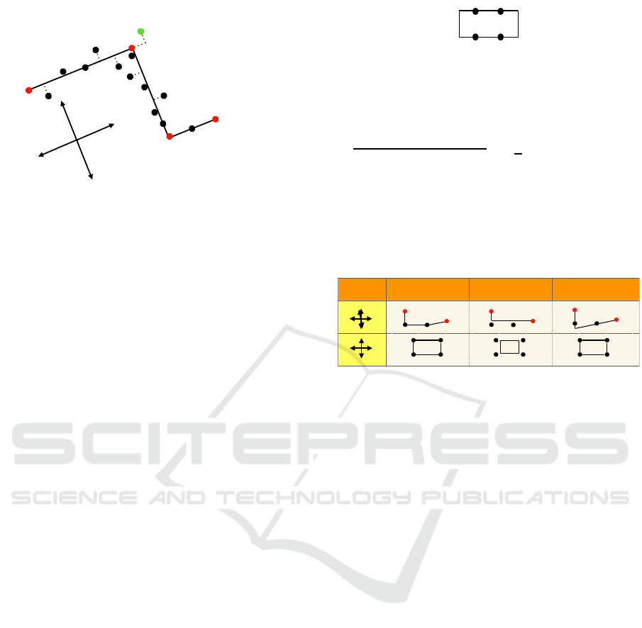
d
+
s
− d
−
s
|
=
|
δ
+
s
− δ
−
s
|
⃗v
s
⃗p
1
⃗p
4
= ⃗p
5
= … = ⃗p
M
⃗r
1
⃗r
2
⃗r
3
= − ⃗r
1
⃗r
4
= − ⃗r
2
⃗p
2
⃗p
3
= ⃗v
S
⃗v
1
=
Figure 1: The dotted lines represent the shortest distances
of points to polyline edges.
objective functions. These non-negative variables are
used to expre ss the distanc e of ~v
s
to the correspond-
ing edge, d
s
= d
+
s
−d
−
s
, and for an optimal solution:
δ
+
s
= δ
−
s
= 0 if the orthogonal projection lies inside
the edge, and δ
+
s
+ δ
−
s
= min{|
˜
λ
s
|,|
˜
λ
s
−L
k
|} other-
wise.
The conditions (5) and (6) only become relevant,
if b
k,s
= a
k,l
= 1. Then normal~r
l
will be assigned to
the edge between ~p
k
and ~p
k+1
, and the direction of
the edg e is given by (−~r
l
.y,~r
l
.x). The given vertex ~v
s
is also assigned to the edge. The c onditions (5) and
(6) are used to compute the point ~p
k
+
˜
λ
s
(−~r
l
.y,~r
l
.x)
that is closest to ~v
s
and lies on the straight line. Since
~r
l
is perpendicular to the line, this point also has a
representation of ~v
s
+ (d
+
s
−d
−
s
)~r
l
, and by solving
these two linear equations (5) and (6) one obtains
˜
λ
s
and d
s
= d
+
s
−d
−
s
. The distance between ~v
s
and the
straight line is |d
+
s
−d
−
s
| and will e qual d
+
s
+ d
−
s
for
an optimal solution.
Note that we cannot use the direction vector ~p
k+1
−~p
k
instead of (−~r
l
.y,~r
l
.x) because we would multi-
ply the structure variables ~p
k+1
and ~p
k
with
˜
λ
s
. Thus,
we would loose linearity.
The no rmal~r
l
assigned to the edge between ~p
k
and
~p
k+1
can be ch osen so that vectors (−~r
l
.y,~r
l
.x) an d
~p
k+1
−~p
k
point in the same direction (constraints (7)
and L
k
≥0), because we have added negative normals
to the initial list of normal vectors. The inner product
between vector s pointing in the same direction is non-
negative, and the length of the edge is given by (7):
L
k
:= (~p
k+1
−~p
k
) ·(−~r
l
.y,~r
l
.x)
= |~p
k+1
−~p
k
||(−~r
l
.y,~r
l
.x)|cos(0) = |~p
k+1
−~p
k
|.
The factor
˜
λ
s
is decomposed into the sum λ
s
+ δ
+
s
−
δ
−
s
. With condition (8), there is λ
s
∈ [0,L
k
]. If and
only if the nearest point lies within the e dge betwee n
~p
k
and ~p
k+1
, the variables δ
+
s
and δ
−
s
become zero.
Otherwise, in conjunction with the objective func-
tions, δ
+
s
+ δ
−
s
is the absolute distance from the clo s-
est point to ~v
s
on the straight line th rough the edge to
Figure 2: Four vertices are connected with a minimum num-
ber of horizontal and vertical edges of a closed polyline.
the nearest endpoint of the edge, see Figure 1. Thus,
for an optimal solution, eac h point ~v
s
is closer to its
associated edge than
q
(d
+
s
−d
−
s
)
2
+ (δ
+
s
−δ
−
s
)
2
≤
√
2max{d
+
s
,d
−
s
,δ
+
s
,δ
−
s
},
because two of the four variables become zero.
For p e rformance reasons, we define SOS 1 sets of
binary variables that sum up to a t most one. For eac h
k ∈[M −1] variables a
k,l
, l ∈[2N], and for each s ∈[S]
variables b
k,s
, k ∈ [M −1], constitute such sets.
normals
min. dist.
min. length
min. edges
Figure 3: The three objective functions lead to different re-
sults: Red vertices are fixed endpoints.
We discuss the following optimization goals for
which Figure 3 shows the principal differences:
1. [min. dist.] Find a po lyline (with a limited num-
ber of vertices) that minimizes a linear combin a -
tion of the distan ces to the given points and its
length. The coefficients α > β > 0 of the linear
combination can be chosen so that the focus is on
the minimization of the distan ces. However, the
length of the polyline must also be considered, so
that the gr aph in Figure 2 will not be an optim al
solution.
minimize
α
S
∑
s=1
(d
+
s
+ d
−
s
+ δ
+
s
+ δ
−
s
) + β
M− 1
∑
k=1
L
k
!
.
(10)
2. [min. le ngth] Find a polyline of minimum length
so that all given points are within a threshold dis-
tance defined by ε > 0. To this end , let d
+
s
,d
−
s
,
δ
+
s
,δ
−
s
≤ ε. Then
minimize
M− 1
∑
k=1
L
k
!
.
However, we also want to minimize the distances
to given points. With (cf. (10))
minimize
GRAPP 2024 - 19th International Conference on Computer Graphics Theory and Applications
206

M− 1
∑
k=1
L
k
!
+
µ
S ·2ε
S
∑
s=1
(d
+
s
+ d
−
s
+ δ
+
s
+ δ
−
s
)
(11)
we find polylines that may slightly exceed the min
length up to µ > 0. But they are generally closer
to the given points. If one deals w ith closed con-
tours, then the objective will result in a polygon
that may be slightly smaller than the given poly-
line, see Figure 3.
3. [min. edges] Find a polyline w ith a minimum
number of edges such that all given points are
within a thresho ld distance defined by ε. Similar
to befo re, among all polylines that meet th ese con-
ditions, we select one that is closest to the given
points. To also count edges, we add constraints
d
+
s
,d
−
s
,δ
+
s
,δ
−
s
≤ ε and
c
k
∈ {0, 1} fo r k ∈ [M −1]
∀
k∈[M−1]
−C(1 −c
k
) ≤~p
k
.x −~p
k+1
.x ≤C(1 −c
k
) (12)
−C(1 −c
k
) ≤~p
k
.y −~p
k+1
.y ≤C(1 −c
k
) (13)
c
k
+
S
∑
s=1
b
k,s
≥ 1. (14)
Then the task is to
maximize
M− 1
∑
k=1
c
k
!
−
1
4Sε
S
∑
s=1
(d
+
s
+ d
−
s
+ δ
+
s
+ δ
−
s
).
(15)
If and only if the consecutive points ~p
k
and ~p
k+1
are equal, ~p
k
= ~p
k+1
, the binary variable c
k
can
and will be set to one, see (12) and (13) in con-
junction with the objective function. The p rimary
optimization go al in (15) is to maximize the nu m-
ber of equal points, i.e., to min imize the num-
ber of vertices of the simplified polyline. As a
secondary objec tive in (15), the sum of the dis-
tances between the given vertices and the edges
of the simplified polyline is minimized. Each of
the S summands is b ounded by ε. Thus, the sum
does not exceed Sε an d its factor limits the size
at 0.5. As a consequen ce, it is more important to
save a vertex then to have edges th a t are closer to
given vertices. However, among all solutions with
a minimum number of vertices, a solution with
edges closest to the given vertice s is chosen (in the
sense of the l
1
-norm realized by the secondary ob-
jective). Without the condition (14), the p olygon
in Figure 2 would be optimal since it is allowed to
use edges that are far away from all sample points.
Figure 4: The first polygon has seven but the second poly-
gon has eight edges. Thus the second layout is not optimal
with respect to (15). However, the second polyline is shorter
than the first one.
To avoid this, (14) prescribes every edge of p os-
itive length to be assigned to a given vertex. In
some tests with the solver GLPK
1
, the running
time was reduced significantly by an additional
constraint to avoid the assignment of given poin ts
with edge s of zer o length:
∀
(k,s)∈[M−1]×[S]
b
k,s
≤ 1 −c
k
.
If one uses too few sample points, an optimal so-
lution may not be the intende d one , see Figure 4.
In general, our goal is to map simple polyline s to
simple po lylines. However, the MIPs do not check
for self-intersections, so complex polylines may oc-
cur. Self-intersection must be correc te d in a post-
processing step.
3 APPLICATION TO ROOF
FACET BOUNDAR IES
We detect roof planes using RANSAC on ALS points
of roof segments with homogeneous gradient direc-
tion. Then we generate a 2D map showing regions
of points belonging to individual roof facets and fill
the map with region growing. Each pixel represents a
square of 10 cm ×10 cm. Then we detect the contours
of the regions and mark the critical points where more
than two facets are adjacent (counting the outside of
the building footprint as a facet). All non-black poin ts
are critical in Figure 5. Points near the intersection
points of th ree or more adjacent roo f planes are iden-
tified with the intersection points. Now, contour seg-
ments between critical points are simplified using the
MIPs. In what follows, we describe how the param-
eters and normals are chosen, see Figure 6 for some
results.
A simpler but somewhat similar MIP approach to
ours is used in (Goebbels and Po hle-Fr¨ohlich, 2017),
where the edges are adjusted to the cadastral foot-
print directions they a re already close to. However,
only existing vertices are moved slightly within given
bounds and the number of edges basically remains
1
GLPK LP/MIP Solver 5.0, http://www.gnu.org/
software/glpk/glpk.html (all websites accessed: September
14, 2023)
Polyline Simplification with Predefined Edge Directions by Mixed Integer Linear Programs
207

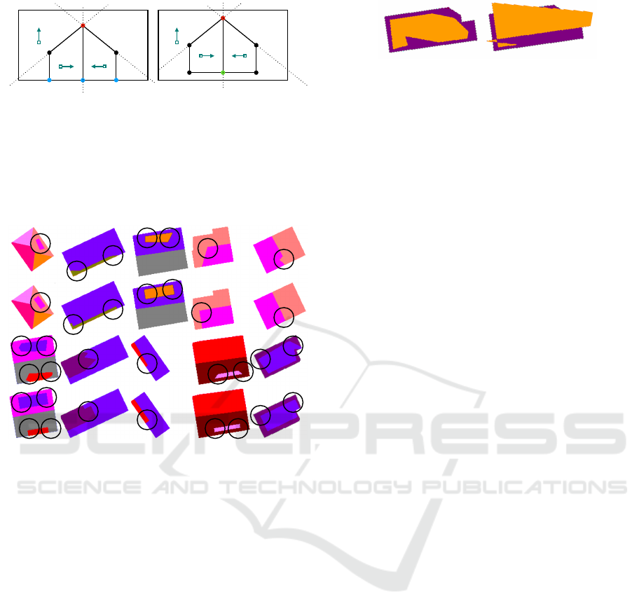
Figure 5: Typical roof, projected onto the 2D ground plane:
A dormer is placed in a surrounding roof facet. The red ver-
tex is an intersection point of three roof planes. Their facets
are adjacent to the vertex. Blue vertices lie on a cadastral
footprint edge. Green is used for other critical points that
are adjacent to more than two facets. Dotted lines corre-
spond with intersection lines between roof planes. Arrows
indicate gradient directions.
Figure 6: Examples for r oof layout si mplification with
ε = 6 pixels. Closed contours were optimized with the
min. edges goal (15) and all other contours were treated
with the min. length objective ( 11).
fixed. Here, we also consider a longest footprint di-
rection and its perpendicular direc tion but only when
a polyline separates two flat roofs. Othe rwise we use
the gradients of non-zero length of the two roof facets
that are separated by the polylin e to be simplified.
We also co nsider their perpendicular directions and
the direction of an in tersection line of the two facet
planes, if it exists. This results in a list of normals~r
l
.
The roof facet bo undaries form a graph. Be-
fore applying optimization proce dures, we reduce the
number o f edges with the Ramer-Douglas-Peucker al-
gorithm while keeping in particular the critical points
as vertices. We discuss several cases:
The first case deals with a clo sed polyline that sep-
arates exactly two roof facets. Ofte n, such a poly-
gon is a rectang le defining a dorme r. This poly-
gon is either simplified by the min. edges or by the
min. dist. objective. Minimizing th e length of the
polyline would result in polygons that are sligh tly too
small, see Figur e 3. The other cases d eal with open
polylines that have critical points as endpoints.
Open polylines can be simplified with any of th e
Figure 7: An example with self-intersection and intersec-
tion with the enclosing building footprint.
three objective functions. We need to determine how
to handle their endpoints.
• An en dpoint must remain in place, if it is an inter-
section point of three or more adja cent roof planes
or a vertex of the cadastral footprint.
• For each other endpoint that lies on a footprint
edge, we add a constraint that the simplified poly-
line must end on that line, cf. (1). In Figure 5, the
blue critical points have to stay on the footprint.
• In our test data (see next section) , the previous two
cases already cover over 90% of the contour seg-
ments that have more than one edge. In principle,
the remaining e ndpoints can be moved. However,
since we are optimizing contour segments itera-
tively, we must avoid undoing improvements that
have already been made. If such a remaining end-
point is used for the first time in an optimization
problem, its coordinates are allowed to vary by ε.
However, if it has already been used, it may be
moved by a maximum of ε on all the straight lines
that lie on the edges where it was the endpoint
in a result of a previous optimization problem. If
an endpoint alrea dy lies on two straight lines with
linearly independent directions, it is fixed.
The position of an end point of an open polyline
may depend on two optimization problems th at are
solved sequentially. This is much faster than solving
combined problems that deal with multiple polylines.
The resulting polylines may have self-intersec-
tions. Also inter sections with boundaries of enclosing
roof facets and the cadastral footprint are possible, see
Figure 7. Such intersections bec ome unlikely if small
distance bounds ε are used, conto urs ar e sampled with
sufficiently many points, and normal vectors fit with
the contour. We generally remove intersections in a
post-processing step.
4 EXPERIMENTS
We evaluated the approach for on e square kilome -
ter of the city center of Krefeld with 5,467 buildings
shown in Figure 8 on a computer with a 2.3 GH z dual-
core Intel Core i5 with 16 GB of RAM. T he corre-
sponding ALS point cloud was provided by GeoBasis
GRAPP 2024 - 19th International Conference on Computer Graphics Theory and Applications
208

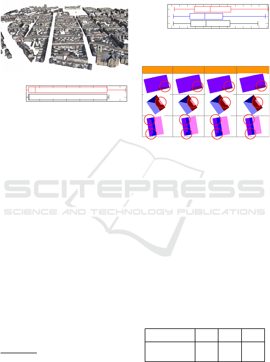
Figure 8: The final 3D model of one square kilometer.
0 10 20 30 40 50 60 70
min. edges
min. dist.
Figure 9: Running times for 111 closed contours with
existing solutions in seconds, red: 111 solutions for the
minimum distances goal (10), black: 95 solutions of the
min. edges objective (15).
NRW
2
. The parameters are set as follows: C = 1000,
α = C, β = ε, µ = 1, ε := 3 pixels. Since we want to
reduce complexity, the maximum number M of poly -
line vertices is chosen to be equal to the number S of
given vertices if the contour is not closed. Otherwise
we set M := S + 1 to ensure that the startpoin t and
endpo int of th e simplified polyline ar e the same. We
have integrated the MIPs into a workflow for cr eating
3D city models using the C-API of the IBM CPLEX
12.8.0. optimizer
3
. Instead of work ing w ith optimal
solutions, we are satisfied with a best solution found
within a time-limit of 60 seconds. This time-limit is
checked with a callback function that is invoked by
CPLEX at irregular time steps. Thu s, running times
may exceed 60 seco nds slightly. The optimization
problems had between 21 and 2,118 variables includ-
ing 6 to 1,813 binary variables. We u sed up to 60,796
constraints.
We simplified 111 closed polylines with the two
objective functions (10) and (15). In 33 a nd 34 prob-
lems, respectively, the time-limit was re ached. Nev-
ertheless, we o btained a feasible solu tion for all of
the problems when minimizing distances with the
min. dist. objective (10) , while no feasible solution
was obtained for 1 6 instances with the min. edges goal
(15). Th e reasons for this behavior are the same as for
open polylines and are discu ssed below. The running
times are comp ared in Figure 9.
Open polylin es had an average o f 18,352 fixed
endpo ints, 38,280 endpoints that were restricted to
2
https://www.bezreg-koeln.nrw.de/geobasis-nrw
3
https://www.ibm.com/de-de/analytics/
cplex-optimizer, the newer C PLEX version 22.1.1
showed almost exactly the same running times
0 0.004 0.008 0.012 0.016
. . .
60 80
min. edges
min. length
min. dist.
Figure 10: Running times for open contours with existing
solutions in seconds, red: minimum distances optimization
with (10), blue: minimum length objective (11), black: min-
imum number of edges goal (15).
input
min. dist.
min. length
min. edges
Figure 11: The three optimization goals may result in
slightly different roof layouts.
vary on edges, and 1,343 endpoints that we re allowed
to move freely with in the coordinate -wise tolerance ε.
Figure 10 compares the running times due to the dif-
ferent objectives. Problems with the min. dist. condi-
tion (10) took sligh tly longer to solve than problems
with the othe r two obje c tives. However, more feasible
solutions were found for this objective (10) than for
the other goals because distances we re not bounded
by ε, see Tab le 1. However, in some examp les this re-
sulted in larger changes which can be avoided by also
requirin g d
+
s
,d
−
s
,δ
+
s
,δ
−
s
≤ ε. In general, the qua lita-
tive results differ only slightly between the chosen o b-
jective functions, see Figure 11. If, unlike in our test
scenario, mod els are created interactively, all three
optimization goals can be offered as tools so that the
best fitting result can be selected.
Table 1: Feasible solutions for polylines with critical end-
points, found with the three objectives; problem instances
that have exceeded the time-limit also contribute to the
rows “feasible solutions” and “no solutions found”. How-
ever, apart from the small number of aborted problems with
reached time-limit, feasible solutions are optimal and “no
solution found” means that the associated problem really
has no solution.
min. min. min.
dist. length edges
feasible solutions 18,331 14,978 15,218
no solution found 10,591 13,665 14,180
time-li mit re ac hed 328 295 256
One reason for the significant number of problem
instances without fe a sible solu tions is that th e con-
Polyline Simplification with Predefined Edge Directions by Mixed Integer Linear Programs
209

tours do not sufficiently match with the pre scribed
directions defined by the roof plane gradients and
their intersections. This can be an effect of the re-
gion growing me thod applied previously. Especially,
it occu rs when small roof facets are not detected
by RANSAC, so that corresponding regions must be
filled with adjacent facets. T he maximum to le rance ε
was chosen to be sma ll eno ugh to avoid inconsisten-
cies, but the behavior does not change if the tolerance
is moderately increased from three to six pixels with-
out increasing the number of vertices M.
5 CONCLUSIONS
We have in troduced MIPs that modify p olylines un-
der directional constraints. The applicability of the
programs has been demonstrated in the context of 3D
modeling of building roofs. In this scenario, we had to
deal with a large number of contours. Therefo re, short
running times of the individual MIPs were important.
Each contour was alrea dy simplified so that it could
be described with a f ew sampled polyline vertices. In
most cases, the MIPs did not reduce the nu mber of
vertices. The maximum reduction was 21 vertices.
This resulted in MIP running times of a few millisec-
onds. When applying the MIPs to polylines with more
vertices, longer running times can be expected.
Polyline simplification based on normals is not
limited to 3D building reconstruction. An everyday
example is p ublic transport maps th at show general-
ized paths instead of exact ones.
ACKNOWLEDGEMENTS
The authors are grateful to Dagmar Schumacher for
proof-reading and to Udo Ha nnok and Philipp Blu-
menkamp from the Krefeld land registry office for
providing us with oblique aerial images.
REFERENCES
˚
Arøe, A. L. (2022). Detection of Edge Points of Building
Roofs from ALS Point Clouds. Norwegian University
of Science and Technology (PhD thesis), Trondheim.
Aronov, B., Asano, T., Katoh, N., Mehlhorn, K., and
Tokuyama, T. (2005). Polyline fitting of planar points
under min-sum criteria. In Fleischer, R. and Trippen,
G., editors, Proc. ISAAC 2004: Algorithms and Com-
putation, volume 3341 of LNCS, pages 77–88, Berlin,
Heidelberg. Springer.
Bode, L., Weinmann, M., and Klein, R. (2022). B oundED:
Neural boundary and edge detection in 3D point
clouds via local neighborhood statistics. arXiv,
arXiv.2210.13305:1–20.
Douglas, D. and Peucker, T. (1973). Algorithms for the re-
duction of the number of points required to represent
a digitized line or its caricature. The Canadian Car-
tographer, 10(2):112–122.
Funke, S., Mendel, T., Miller, A., Storandt, S ., and Wiebe,
M. (2017). Map simplification with topology con-
straints: Exactly and in practice. In Fekete, S.
and Ramachandran, V., editors, Proc. 19th Workshop
on Algorithm Engineering and Experiments 2017
(ALENEX17), pages 185–196, Red Hook, NY. Curran
Associates.
Goebbels, S. and Pohle-Fr¨ohlich, R. (2017). Quality en-
hancement techniques for building models derived
from sparse point clouds. In Proc. 12th International
Joint Conference on Computer Vision, Imaging and
Computer Graphics Theory and Applications – Vol-
ume 1: GRAPP, (VISIGRAPP 2017), pages 93–104.
INSTICC, SciTePress.
Gr¨oger, G., Kolbe, T. H ., Nagel, C., and H¨afele, K. H.
(2012). OpenGIS City Geography Markup Language
(CityGML) Encoding Standard. Version 2.0.0. Open
Geospatial Consortium.
Imai, H. and Iri, M. (1986). An optimal algorithm for ap-
proximating a piecewise linear function. Journal of
Information Processing, 9(3):159–162.
Lang, T. (1969). Rules for r obot draughtsmen. The Geo-
graphical Magazine, 42(1):50–51.
Li, L., Songa, N., Sun, F., Liu, X. , Wang, R., Yaoa, J., and
Cao, S. (2022). P oint2roof: End-to-end 3D building
roof modeling from airborne LiDAR point clouds. IS-
PRS Journal of Photogrammetry and Remote Sensing,
193:17–28.
Nauata, N. and Furukawa, Y. (2020). Vectorizing world
buildings: Pl anar graph reconstruction by primitive
detection and relationship inference. In Vedaldi,
A., Bischof, H., Brox, T., and Frahm, J., editors,
Proc. Computer Vision–ECCV 2020: 16th Euro-
pean Conference, Part VIII, number 12353 in LNCS,
Cham. Springer.
Pinheiro, A. M. G. and Ghanbari, M. (2010). Piecewise
approximation of contours through scale-space selec-
tion of dominant points. IEEE Transactions on Image
Processing, 19(6):1442–1450.
Ramer, U. (1972). An iterative procedure f or the polygonal
approximation of plane curves. Computer Graphics
and Image Processing, 1(3):244–256.
Reumann, K. and Witkam, A. (1973). Optimizing curve
segmentation in computer graphics. In Gunther, A.,
Levrat, B., and Lipps, H., editors, Proc. International
Computing Symposium, Davos, pages 467–472, New
York, NY. Elsevier.
Visvalingam, M. and Whyatt, J. D. (1992). Line generalisa-
tion by repeated elimination of the smallest area. Car-
tographic Information Systems Research Group, Uni-
versity of Hull.
Zhao, Z. and Saalfeld, A. (1997). Linear-time sleeve-fitting
polyline simplification algorithms. In Proc. AutoCarto
13, Seattle, WA, pages 214–223, Maryland. American
Congress on Surveying and Mapping & American So-
ciety for Photogrammetry and Remote Sensing.
GRAPP 2024 - 19th International Conference on Computer Graphics Theory and Applications
210