Variance Reduction of Resampling for Sequential Monte Carlo

Xiongming Dai

and Gerald Baumgartner

Division of Computer Science and Engineering, Louisiana State University, Baton Rouge, 70803, LA, U.S.A.

Keywords:

Resampling, Sequential Monte Carlo, Hidden Markov Model, Repetitive Ergodicity, Deterministic Domain.

Abstract:

A resampling scheme provides a way to switch low-weight particles for sequential Monte Carlo with higher-

weight particles representing the objective distribution. The less the variance of the weight distribution is, the

more concentrated the effective particles are, and the quicker and more accurate it is to approximate the hidden

Markov model, especially for the nonlinear case. Normally the distribution of these particles is skewed, we

propose repetitive ergodicity in the deterministic domain with the median for resampling and have achieved the

lowest variances compared to the other resampling methods. As the size of the deterministic domain M ≪ N

(the size of population), given a feasible size of particles under mild assumptions, our algorithm is faster than

the state of the art, which is veriﬁed by theoretical deduction and experiments of a hidden Markov model in

both the linear and non-linear cases.

1 INTRODUCTION

Sequential Monte Carlo (SMC) or Particle Fil-

ter (Gordon et al., 1993) is a set of Monte Carlo

methods for solving nonlinear state-space models

given noisy partial observations, which are widely

used in signal and image processing (S

arkk

a et al.,

2007), stock analysis (Casarin et al., 2006; Flury

and Shephard, 2011; Dai and Baumgartner, 2023a;

Dai and Baumgartner, 2023d), Bayesian inference

(Del Moral et al., 2006; Dai and Baumgartner, 2023b;

Dai and Baumgartner, 2023c) or robotics (Fox, 2001;

Montemerlo et al., 2002; Thrun, 2002). It updates

the predictions recursively by samples composed of

weighted particles to infer the posterior probability

density. While the particles will be impoverished as

the sample forwards recursively, it can be mitigated

by resampling where the negligible weight particles

will be replaced by other particles with higher weights

(Doucet et al., 2000; Del Moral et al., 2012; Doucet

et al., 2001).

In the literature, several resampling methods and

corresponding theoretical analysis (K

unsch et al.,

2005; Chopin et al., 2004; Douc and Moulines, 2007;

Gilks and Berzuini, 2001) can be found. The fre-

quently used algorithms are residual resampling (Liu

and Chen, 1998), multinomial resampling (Gordon

et al., 1993), stratiﬁed resampling (Smith, 2013),

https://orcid.org/0009-0001-8540-3276

https://orcid.org/0009-0007-1162-159X

and systematic resampling (Kitagawa, 1996; Arulam-

palam et al., 2002). A justiﬁed decision regarding

which resampling strategies to use might result in a

reduction of the overall computation effort and high

accuracy of the estimations of the objective. How-

ever, for resampling, most of these strategies traverse

repetitively from the original population, the negligi-

ble weight particles fail to be discarded completely,

although the diversity of the particle reserve, it causes

unnecessary computational load for a very heavily

skewed distribution of particles and affects the accu-

racy of estimations of the posterior distribution. From

the perspective of complexity and variance reduction

with promising estimation, we propose a repetitive

deterministic domain ergodicity strategy, where more

concentrated and effective particles are drawn to ap-

proximate the objective. Our proposal can be widely

used in large-sample approximations.

In this paper, we concentrate on the analysis of

the importance sample resamplings built-in SMC for

the hidden Markov model. In Section 2, we present a

brief introduction to SMC. Here, a brief introduction

to the hidden Markov model and the sequential im-

portance sampling method will be given. Our method

will be introduced in Section 3, where we introduce

the origin of our method, and how to implement each

step in detail, and then the theoretical asymptotic be-

havior of approximations using our method is pro-

vided. The practical experiments will be validated by

Section 4, where performance and complexity analy-

Dai, X. and Baumgartner, G.

Variance Reduction of Resampling for Sequential Monte Carlo.

DOI: 10.5220/0012252100003636

Paper published under CC license (CC BY-NC-ND 4.0)

In Proceedings of the 16th International Conference on Agents and Artiﬁcial Intelligence (ICAART 2024) - Volume 3, pages 34-41

ISBN: 978-989-758-680-4; ISSN: 2184-433X

sis are presented. The summary of our contributions

is outlined in Section 5.

2 RESAMPLING IN SMC FOR

HIDDEN MARKOV MODEL

Consider the state-space model, which is also known

as a hidden Markov model, described by

| X

t−1

∼ f (X

| X

t−1

), Y

| X

∼ g(y

| X

). (1)

The initial state X

∼ µ(X

), X

,(t = 1,2,...n) is

a latent variable to be observed, the measurements Y

are assumed to be conditionally independent given X

the most objective is to estimate X

The recursive Bayesian estimation can be used

and it is described as:

(a) Prediction:

π(X

| y

1:t−1

) =

f (X

| X

t−1

)π(X

t−1

| y

1:t−1

)dX

t−1

(2)

(b) Update:

π(X

| y

1:t

) =

g(y

| X

)π(X

| y

1:t−1

)

g(y

| X

)π(X

| y

1:t−1

)dX

. (3)

From (2) and (3) the integral part is unreachable,

especially, for high-dimensional factors involved, we

fail to get the close form of π(X

1:t

) (S

arkk

a, 2013;

Doucet and Johansen, 2009).

Sequential Monte Carlo is a recursive algorithm

where a cloud of particles are propagated to approx-

imate the posterior distribution π(X

0:t

| y

1:t

). Here,

we describe a general algorithm that generates at time

t, N particles

(i)

0:t

i=1

with the corresponding em-

pirical measure

π(X

0:t

| y

1:t

) =

∑

i=1

(i)

0:t

(dX

0:t

), a

discrete weighted approximation of the true posterior

π(X

0:t

1:t

), δ

(i)

0:t

(dX

0:t

) denotes the delta-Dirac mass

located at X

, dX

0:t

equals to X

0:t

−X

0:t

. The particles

are drawn recursively using the observation obtained

at time t and the set of particles

(i)

0:t−1

i=1

drawn

at time t −1, accordingly, where

π(X

0:t−1

| y

1:t−1

) ≈

π(X

0:t−1

| y

1:t−1

). The weights are normalized us-

ing the principle of importance sampling such that

∑

i=1

= 1. If the samples X

0:t

are drawn from an

importance density q(X

0:t

| y

1:t

), we have

∝

π(X

0:t

| y

1:t

)

q(X

0:t

| y

1:t

)

. (4)

Suppose at time step t −1, we have existed sam-

ples to approximate the current posterior distribution

π(X

0:t−1

| y

1:t−1

), if we get a new observation y

time t, a recursive approximation to π(X

0:t

| y

1:t

) with

a new set of samples can be obtained by importance

sampling, the corresponding factorization (Arulam-

palam et al., 2002) is described by

q(X

0:t

| y

1:t

) := q(X

| X

0:t−1

1:t

)q(X

0:t−1

| y

1:t−1

(5)

Then, we can get the new samples X

0:t

∼ q(X

0:t

1:t

) by propagating each of the existing samples

0:t−1

∼q(X

0:t−1

t−1

) with the new state X

∼q(X

0:t−1

). To derive the weight update equation, we

follow the ergodic Markov chain properties of the

model, the full posterior distribution π(X

0:t

| y

1:t

) can

be written recursively in terms of π(X

0:t−1

| y

1:t−1

g(y

) and f (X

t−1

) (Arulampalam et al., 2002):

π(X

0:t

| y

1:t

) =

p(y

| X

0:t

1:t−1

)p(X

0:t

| y

1:t−1

)

p(y

| y

1:t−1

)

1:t

∝ g(y

| x

) f (x

| x

t−1

)π

1:t−1

(6)

where π

1:t

is short for π(X

0:t

| y

1:t

). By substituting

(5) and (6) into (4), we have

∝

g(y

| X

) f (X

| X

t−1

)p(X

0:t−1

| y

1:t−1

)

q(X

| X

0:t−1

1:t

)q(X

0:t−1

1:t−1

)

= w

t−1

g(y

| X

) f (X

| X

t−1

)

q(X

| X

0:t−1

1:t

)

(7)

We assume the state X

is ergodic Markovian, thus,

= q(X

| X

0:t−1

1:t

) = q(X

| X

t−1

), from this

point, we only need to store the X

, and obtain the

thinning recursively update weight formula (Gordon

et al., 2004):

∝ w

t−1

g(y

| x

) f (x

| x

t−1

)

q(x

| x

t−1

)

. (8)

The corresponding empirical posterior ﬁltered density

π(X

| y

1:t

) can be approximated as

π(X

| y

1:t

) =

∑

i=1

(i)

(dX

). (9)

It can be shown that as N → ∞,

π(X

| y

1:t

) con-

verges to π(X

| y

1:t

Ideally, the importance density function should

be the posterior distribution itself, π(X

0:t

| y

1:t

). The

variance of importance weights increases over time,

which will decrease the accuracy and lead to degener-

acy that some particles make up negligible normal-

ized weights. The brute force approach to reduc-

ing the effect of degeneracy is to increase N as large

as possible. However, as the size of the sample in-

creases, the computation of the recursive step will

Variance Reduction of Resampling for Sequential Monte Carlo

also be exponentially costly. Generally, we can try

two ways to improve: (I) suitable importance density

sampling; (II) resampling the weights. Here we fo-

cus on the latter. A suitable measure of the degener-

acy of an algorithm is the effective sample size N

eff

introduced in (Arulampalam et al., 2002): N

eff

1+Var(w

∗i

)

, w

∗i

π(X

1:t

)

q(X

t−1

)

, while the close solu-

tion is unreachable, it could be approximated (Liu,

2008) by

eff

∑

i=1

)

. If the weights are uniform,

for each particle i = 1, 2,..., N, N

eff

= N; If

there exists the unique particle, whose weight is 1, the

remaining are zero, N

eff

= 1. Hence, small N

eff

eas-

ily leads to a severe degeneracy (Gordon et al., 2004).

We use

eff

as an indicator to measure the condition

of resampling for our experiments in section 4.

We will introduce our proposal based on the repet-

itive deterministic domain traverse in the next section.

3 REPETITIVE ERGODICITY IN

DETERMINISTIC DOMAIN

WITH MEDIAN FOR

RESAMPLING

3.1 Multinomial Sampling

A Multinomial distribution provides a ﬂexible frame-

work with parameters p

,i = 1,..., k and N, to mea-

sure the probability that each class i ∈ 1, ...,k has

been sampled N

times over N categorical indepen-

dent tests. It can be used to resample the tag in our

proposal in two steps. Firstly, we obtain the samples

from a uniform generator u

∼ U(0, 1],i = 1, ...,N;

secondly, we evaluate the index j of samples with

the generalized inverse rule, if the cumulative sum of

samples

∑

i=1

larger or equal to u

, this index j will

be labeled, then the corresponding sample w

will be

resampled, this event can be mathematically termed

as g

′

) = I

3.2 Deterministic Domain Construction

The population of weights is divided into two parts.

The ﬁrst part is the weights, larger than the average

, they are considered as the candidate ﬁrstly to

be sampled, we keep r



N ˆw



replicates of ˆw

for each i, where ˆw

is the renormalized unit. r

will be ﬁltered one by one from the population,

and the corresponding tag j will be saved into an

array. We ﬁnd, this part also follows the multinomial

distribution W

∼ Multinomial(M; ˆw

,... ˆw

), We

extract the samples from the population with the

rule of multinomial sampling shown in section 3.1.

This step is the ﬁrst layer of the traverse from the

population, we achieve the ancestor subset. Since the

distribution of these particles is very heavily skewed,

we extract the median of these particles to add to the

set of descendant particles. Then, we renormalized

the weights in the subset, and traverse again to

differentiate the larger weights and other units, until

we get the feasible size of the set to be considered

as the potential deterministic domain. The particles

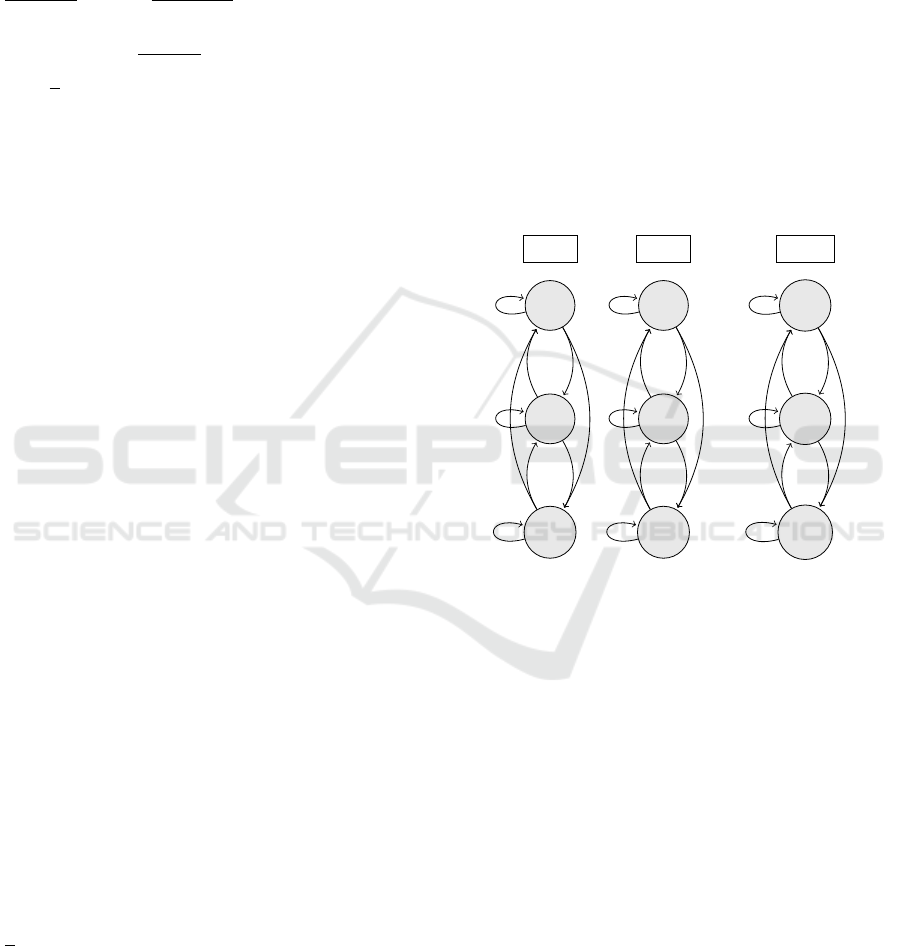
in this domain follow a very strict Markovian, the

evolution can be expressed as follows, where w

denotes the weight corresponding to the particle

(N)

at t.

t = 1

t = 2

t = T

T 2

T 1

T N

···

We deﬁne the integer part event, g

′

( ˆw

) = I

ˆw

= ˆw

similarly for the following repetitive part, ¯g( ¯w

) =

¯w

= ¯w

. We count the units involved in the occurrence

of the event g

′

( ˆw

) and ¯g( ¯w

), then extract these units

based on the tags j, which forms the ﬁnal determinis-

tic domain.

3.3 Repetitive Ergodicity in

Deterministic Domain with Median

Schema

Our goal is to retract and retain units with large

weights, while the remaining ones with low weights

can be effectively replaced in the populations. We set

the desired number of resampled units as the size of

populations under the premise of ensuring unit diver-

sity as much as possible.

We normalized all the units to keep the same

scaled level for comparison, after that, the units with

higher weights above the average level will appear as

real integers (larger than zero) by Ns = ﬂoor(N. ∗w),

ICAART 2024 - 16th International Conference on Agents and Artiﬁcial Intelligence

the remaining will be ﬁltered to zero. This is the pre-

requisite for the deterministic domain construction. In

Ns subset, there exist multiple categorical units, that

follow the multinomial distribution. We sample these

termed large units with two loops, the outer loop is to

bypass the index of the unit zero, and the inner loop

is to traverse and sample the subset where different

large units distribute, there more large weights will

be sampled multiple times.

The last procedure is to repetitively traverse in

the deterministic domain with median, where each

unit will be renormalized and the corresponding cu-

mulative summation is used to ﬁnd the index of the

unit with the rule of the inverse cumulative distribu-

tion function. Each desired unit will be drawn by the

multinomial sampler to rejuvenate the population re-

cursively. The complexity of our method is O(M). As

the size of the deterministic domain M ≪ N (the size

of population), given a feasible size of particles, our

algorithm is faster than the state of the art. The total

implement schema is shown in Algorithm 1.

3.4 Theoretical Asymptotic Behavior of

Approximations

3.4.1 Central Limit Theorem

Suppose that for each t ∈ [1,T ],

(1)

,...,

(M)

are in-

dependent, where

′

)

′

∈ [1,M] denotes the me-

dian of the originator particles. For others

(i)

,i ̸= m

′

belong to the deterministic domain; the probability

space of the sequence recursively changes with t for

sequential Monte Carlo, such a collection is called a

triangular array of particles. Let S

(1)

+ ... +

(M)

. We expand the characteristic function of each

(i)

to second-order terms and estimate the remainder

to establish the asymptotic normality of S

. Suppose

that both the expectation and the variance exist and

are ﬁnite:

(i)

) =

∈Ω

(i)

(dX

)q(X

,dX

t+1

) < ∞,

t,i

(i)

) = E[(X

(i)

−E(X

(i)

))

] < ∞.

(10)

Theorem 1 For each t the sequence

(1)

,...,

(M)

sampled from the originator particles X

(1)

,..., X

(N)

suppose that are independent, where

′

)

′

∈[1,M]

denotes the median of the originator particles. For the

rest

(i)

,i ̸= m

′

belong to the deterministic domain;

let Ψ be a measurable function and assume that there

Input: The input weight sequence:w; the

desired number of resampled

particles: N

Output: The resampled tag of the weight

sequence tag

if nargin==1 then

N ← length(w); // Desired size

end

M ← length(w);

w ← w/sum(w); // Normalization

tag ←zeros(1,N);

Ns ← ﬂoor(N. ∗w); // Integer parts

R ← sum(Ns);

i ← 1; // Extract deterministic part

j ← 0;

while j < M do

j ← j + 1;

count ← 1;

while count <= Ns(j) do

tag(i) ← j;

i ← i + 1;

count ← count + 1;

end

[W,I] = sort(w); // Median extraction

r = f loor((N + 1)/2);

tag(i) = I(r);

i = i + 1; // Deterministic domain

w ←tag/sum(tag);

q ← cumsum(w)

while i<=N do

sampl ← rand;

j ← 1;

while q(j)<sampl do

j ← j + 1; // Update the tag

end

tag(i) ←tag( j);

i ← i + 1;

end

Algorithm 1: Repetitive Deterministic Domain with

Median Traversal Resampling.

exists

⊂ K satisfying

x∈K

π(dx)E

∑

t=1

Ψ(X

)

2+ε

< ∞ (11)

and

sup

x∈K

∑

t=1

Ψ(X

)

< ∞,

[Ψ] :=

π(dx)E

∑

i=1

Ψ(X

(i)

)

< ∞.

(12)

is aperiodic, irreducible, positive Harris recur-

rent with invariant distribution π and geometrically

Variance Reduction of Resampling for Sequential Monte Carlo

ergodic, and if, in addition,

t,i

(Ψ) :=

π(dx)E





Ψ(

(i)

) −E

[Ψ]





< ∞,

:= lim

M→∞

∑

i=1

t,i

(Ψ),

(13)

{Ψ(

(i)

} satisﬁes

lim

M→∞

∑

i=1

Ψ(

(i)

) −E

[Ψ]

∼ N(0, s

). (14)

Proof Let Y

t,i

= Ψ(

(i)

) − E

[Ψ], by (Billingsley,

1995),



−

∑

k=0

(iy)



≤ min{

(y)

M+1

(M+1)!

2(y)

}, when

M = 2, we have



−(1 + iy −

)



≤ min{

}. (15)

We ﬁrst assume that Ψ(·) is bounded, from

the property of characteristic function, the left-hand

side can be written as



(iλY

t,i

)

−(1 −

t,i

(Ψ)

)



therefore, the corresponding character function

t,i

(λ) of Y

t,i

satisﬁes



t,i

(λ) −(1 −

t,i

(Ψ)

)



≤ E

min{

λY

t,i

λY

t,i

}

(16)

Note that the expected value exists and is ﬁnite, the

right-hand side term can be integrated by

t,i

≥εδ

t,i

√



min{

λY

t,i

λY

t,i

}



dx. (17)

As M → +∞,{Y

t,i

} →

0, then,

min{

λY

t,i

λY

t,i

}

→ 0, which satisﬁes

Lindeberg condition:

lim

M→∞

∑

i=1

t,i

≥εδ

t,i

√

t,i

dX = 0, (18)

for ε > 0,s

∑

i=1

t,i

(Ψ).

lim

M→∞



t,i

(λ) −(1 −

t,i

(Ψ)

)



= 0. (19)

By (26.11) in page 345 (Billingsley, 1995),

t,i

(λ) = 1 + iλE[X] −

E[X

] + o(λ

),λ → 0.

(20)

By Lemma 1 in page 358 (Billingsley, 1995),



∏

i=1

−λ

t,i

(Ψ)/2

−

∏

i=1

(1 −

t,i

(Ψ))



≤

∑

i=1



−λ

t,i

(Ψ)/2

−1 +

t,i

(Ψ)



≤

∑

i=1

t,i

(Ψ)

∞

∑

j=2

j−2

2 j−4

t,i

(Ψ)

≤

∑

i=1

t,i

(Ψ)e

t,i

(Ψ)

(21)

Thus,

∏

i=1

−λ

t,i

(Ψ)/2

∏

i=1

(1 −

t,i

(Ψ)) + o(λ

)

∏

i=1

−λ

t,i

(Ψ)/2

+ o(λ

)

= e

−

+ o(λ

(22)

The characteristic function

∏

i=1

t,i

(λ) of

∑

i=1

t,i

∑

i=1

Ψ(X

(i)

) −E

[Ψ]

is equal to

−

, thus, (14) holds.

4 EXPERIMENTS

In this part, the results of the comparison of these re-

sampling methods are validated from the experiments

with the linear Gaussian state space model and non-

linear state space model, respectively. We ran the ex-

periments on an HP Z200 workstation with an Intel

Core i5 and an #82 −18.04.1− Ubuntu SMP kernel.

4.1 Linear Gaussian State Space Model

This linear model is expressed by:

∼ µ(X

| X

t−1

∼ N(X

;φX

t−1

,δ

| X

∼ N(y

,δ

(23)

we keep parameters the same as (Dahlin and

Sch

on, 2019) to compare with the different resam-

pling methods. Where θ =

{

φ,δ

,δ

}

,φ ∈ (−1,1) de-

scribes the persistence of the state, while δ

,δ

denote

the standard deviations of the state transition noise

and the observation noise, respectively. The Gaus-

sian density is denoted by N(x; µ,δ

) with mean µ and

standard deviation δ > 0. In Figure 1, we use 20 par-

ticles to track the probability distribution of the state,

ICAART 2024 - 16th International Conference on Agents and Artiﬁcial Intelligence

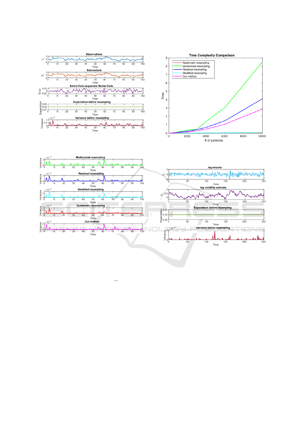
Figure 1: Repetitive deterministic traverse resampling for

linear Gaussian state space model.

Figure 2: Variance analysis for different resampling strate-

gies (note the different scales in the Variance axis).

composed of 100 different times, the ground truth is

from the Kalman ﬁlter (Welch et al., 1995), the er-

ror denotes the difference between the estimation by

SMC and the ground truth. Initially, the expectation

of weights for 20 particles is equal to

, which means

that these particles have equal functions to track the

state.

For the resampling procedure, we compare the

variance from different classical resampling methods,

shown in Figure 2. The variance from the determin-

istic traverse method is the smallest. Thus, the effec-

tive particles are more concentrated after resampling

based on our proposal.

The computational complexity is another factor

the resampling algorithms are compared on, Figure 3

shows the execution times for different particles dis-

tributed, generally, it depends on the machines and

random generator, during our simulations, the time

consumption is different under the same condition of

resampling method and number of particles. Further-

Figure 3: Time complexity analysis for different resampling

strategies.

Figure 4: (a) The daily log-returns. (b) The estimated log-

volatility with 95% conﬁdence intervals of the NASDAQ

OMXS30 index for the period from January 2, 2015 to Jan-

uary 2, 2016. (c) The expectation of weights for particles

before resampling. (d)The variance of weights for particles

before resampling.

more, we ﬁnd under the same resampling methods,

the time consumed for the small size of particles is

much more than that of the larger ones. The compu-

tational stability of particles with resampling methods

is very sensitive to the units from a speciﬁc popula-

tion. For safety, we conduct multiple experiments to

achieve the general complexity trend.

In Figure 3, all the experiments are conducted un-

der the same conditions, for large-size particles, the

stratiﬁed and systematic strategies are favorable. In

Table 1, we can ﬁnd under small-size particles(less

than 150), our method performs best.

Variance Reduction of Resampling for Sequential Monte Carlo

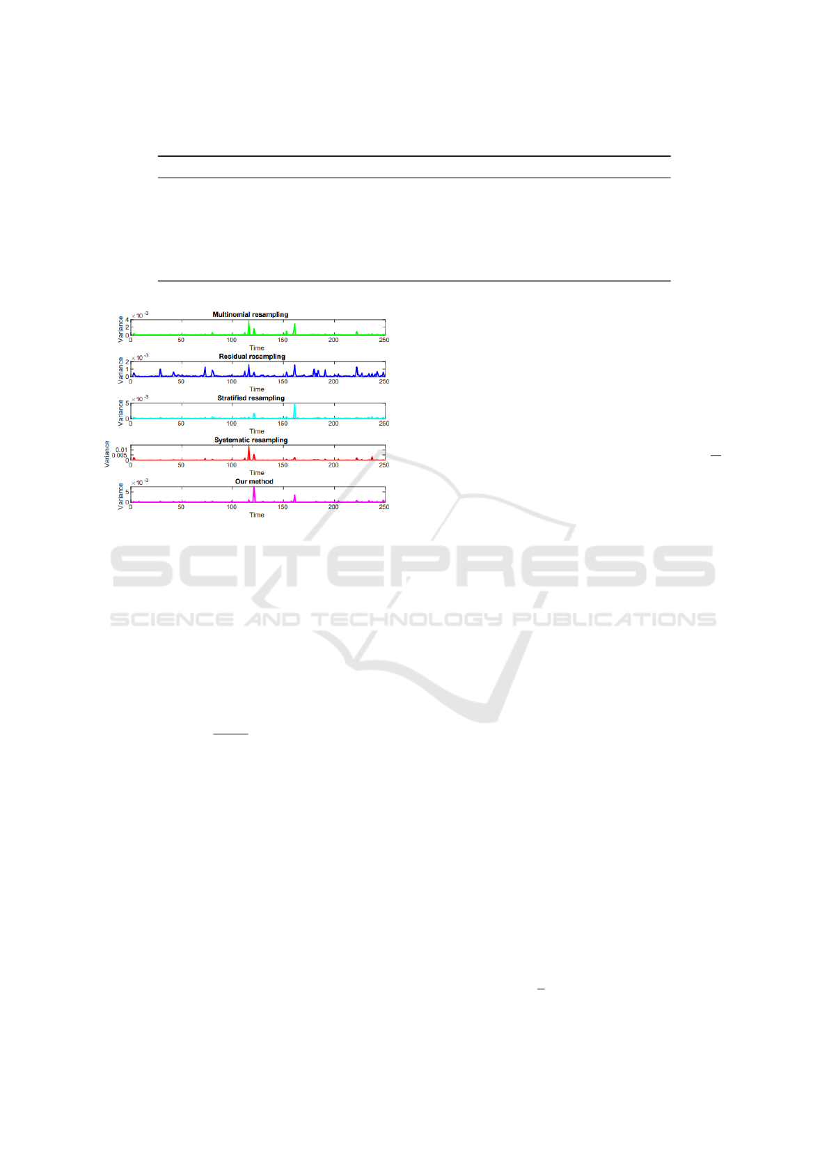
Table 1: Time complexity analysis of different resampling strategies.

# of particles Multinomial resampling Residual resampling Systematic resampling Stratiﬁed resampling Our method

5 0.0026 0.0021 0.0019 0.0023 0.0016

15 0.0036 0.0025 0.0022 0.0033 0.0018

50 0.0057 0.0027 0.0024 0.0047 0.0022

80 0.0087 0.0032 0.0029 0.0051 0.0027

100 0.0127 0.0038 0.0034 0.0067 0.0030

150 0.0161 0.0043 0.0038 0.0088 0.0036

Figure 5: Variance analysis of different resampling strate-

gies for nonlinear state space model (note the different

scales in the Variance axis).

4.2 Nonlinear State Space Model

We continue with a real application of our proposal to

track the stochastic volatility, a nonlinear State Space

Model with Gaussian noise, where log volatility con-

sidered as the latent variable is an essential element

in the analysis of ﬁnancial risk management. The

stochastic volatility is given by

∼ N(µ,

1 −ρ

| X

t−1

∼ N(µ + ρ(X

t−1

−µ),σ

| X

∼ N(0, exp(X

)τ),

(24)

where the parameters θ =

{

µ,ρ,σ

,τ

}

, µ ∈ R,ρ ∈

[−1,1], σ

and τ ∈ R

, denote the mean value, the

persistence in volatility, the standard deviation of the

state process and the instantaneous volatility, respec-

tively.

The observations y

= log(p

t−1

), also called

log-returns, denote the logarithm of the daily differ-

ence in the exchange rate p

, here, {p

}

t=1

is the

daily closing price of the NASDAQ OMXS30 index

(a weighted average of the 30 most traded stocks

at the Stockholm stock exchange). We extract the

data from Quandl for the period between January 2,

2015 and January 2, 2016. The resulting log-return

is shown in Figure 4. We use SMC to track the time-

series persistency volatility, large variations are fre-

quent, which is well-known as volatility clustering in

ﬁnance, from the equation (42), as |φ|is close to 1 and

the standard variance is small, the volatility clustering

effect easier occurs. We keep the same parameters

as (Dahlin and Sch

on, 2019), where µ ∼ N(0,1),φ ∼

T N

[−1,1]

(0.95,0.05

), δ

∼ Gamma(2,10), τ = 1.

We use 25 particles to track the persistency volatil-

ity, the expectation of weights of particles is

shown in Figure 4, it is stable as the same with Fig-

ure 1, the variance is in 10

−3

orders of magnitude un-

der random sampling mechanism.

In Figure 5, the variance from our proposal shows

the minimum value at different times, nearly all the

plots share the common multimodal feature at the

same time, it stems from the multinomial distribution

that both of them have when they resample a new unit.

5 CONCLUSIONS

Resampling strategies are effective in Sequential

Monte Carlo as the weighted particles tend to de-

generate. However, we ﬁnd that the resampling also

leads to a loss of diversity among the particles. This

arises because in the resampling stage, the samples

are drawn from a discrete multinomial distribution,

not a continuous one. Therefore, the new samples

fail to be drawn as a type that has never occurred

but stems from the existing samples by the repetitive

schema. We have presented a repetitive determinis-

tic domain with median traversal for resampling and

have achieved the lowest variances compared to other

resampling methods. As the size of the deterministic

domain M ≪N (the size of population), our algorithm

is faster than the state of the art, given a feasible size

of particles, which is veriﬁed by theoretical deduction

and experiments of the hidden Markov model in both

the linear and the non-linear case.

There is a special case in which the median of par-

ticles belong to a deterministic domain, the particles

with weight ˜w

≤

have been discarded, thus, the

ICAART 2024 - 16th International Conference on Agents and Artiﬁcial Intelligence

particle set after resampling is biased. Since the re-

sampling scheme is repeated in the scaling domain,

the skewed particles are discarded completely, al-

though the total variance obtained by our method is

minimized compared to other resampling methods.

Since these sample points are biased when used for

target tracking, it will affect the accuracy of the tar-

get to some extent. Alternatively, if we give a certain

permissible error threshold for target localization and

tracking, we can also try the feasibility of our method

in this threshold, because it will be solved in a shorter

time with the minimum total variance compared to

other methods.

The broader impact of this work is that it can

speed up existing sequential Monte Carlo applications

and allow more precise estimates of their objectives.

There are no negative societal impacts, other than

those arising from the sequential Monte Carlo appli-

cations themselves.

REFERENCES

Arulampalam, M. S., Maskell, S., Gordon, N., and Clapp,

T. (2002). A tutorial on particle ﬁlters for on-

line nonlinear/non-Gaussian Bayesian tracking. IEEE

Transactions on Signal Processing, 50(2):174–188.

Billingsley, P. (1995). Measure and probability.

Casarin, R., Trecroci, C., et al. (2006). Business Cycle and

Stock Market Volatility: A Particle Filter Approach.

Universit

a degli studi, Dipartimento di scienze eco-

nomiche.

Chopin, N. et al. (2004). Central limit theorem for se-

quential Monte Carlo methods and its application to

Bayesian inference. Annals of Statistics, 32(6):2385–

2411.

Dahlin, J. and Sch

on, T. B. (2019). Getting started with

particle Metropolis-Hastings for inference in nonlin-

ear dynamical models. Journal of Statistical Software,

88(2):1–41.

Dai, X. and Baumgartner, G. (2023a). Chebyshev particles.

arXiv preprint arXiv:2309.06373.

Dai, X. and Baumgartner, G. (2023b). Operator-

free equilibrium on the sphere. arXiv preprint

arXiv:2310.00012.

Dai, X. and Baumgartner, G. (2023c). Optimal camera con-

ﬁguration for large-scale motion capture systems.

Dai, X. and Baumgartner, G. (2023d). Weighted Riesz par-

ticles. arXiv preprint arXiv:2312.00621.

Del Moral, P., Doucet, A., and Jasra, A. (2006). Sequential

monte carlo samplers. Journal of the Royal Statistical

Society Series B: Statistical Methodology, 68(3):411–

436.

Del Moral, P., Doucet, A., and Jasra, A. (2012). On adap-

tive resampling strategies for sequential monte carlo

methods.

Douc, R. and Moulines, E. (2007). Limit theorems

for weighted samples with applications to sequential

Monte Carlo methods. In ESAIM: Proceedings, vol-

ume 19, pages 101–107. EDP Sciences.

Doucet, A., De Freitas, N., Gordon, N. J., et al. (2001). Se-

quential Monte Carlo methods in practice, volume 1.

Springer.

Doucet, A., Godsill, S., and Andrieu, C. (2000). On se-

quential Monte Carlo sampling methods for Bayesian

ﬁltering. Statistics and Computing, 10(3):197–208.

Doucet, A. and Johansen, A. M. (2009). A tutorial on parti-

cle ﬁltering and smoothing: Fifteen years later. Hand-

book of Nonlinear Filtering, 12(656-704):3.

Flury, T. and Shephard, N. (2011). Bayesian inference

based only on simulated likelihood: particle ﬁlter

analysis of dynamic economic models. Econometric

Theory, pages 933–956.

Fox, D. (2001). Kld-sampling: Adaptive particle ﬁlters and

mobile robot localization. Advances in Neural Infor-

mation Processing Systems (NIPS), 14(1):26–32.

Gilks, W. R. and Berzuini, C. (2001). Following a moving

target—Monte Carlo inference for dynamic Bayesian

models. Journal of the Royal Statistical Society: Se-

ries B (Statistical Methodology), 63(1):127–146.

Gordon, N., Ristic, B., and Arulampalam, S. (2004). Be-

yond the Kalman ﬁlter: Particle ﬁlters for tracking ap-

plications. Artech House, London, 830(5):1–4.

Gordon, N. J., Salmond, D. J., and Smith, A. F. (1993).

Novel approach to nonlinear/non-Gaussian Bayesian

state estimation. In IEE Proceedings F (Radar and

Signal Processing), volume 140, pages 107–113. IET.

Kitagawa, G. (1996). Monte Carlo ﬁlter and smoother for

non-Gaussian nonlinear state space models. Journal

of Computational and Graphical Statistics, 5(1):1–25.

unsch, H. R. et al. (2005). Recursive Monte Carlo ﬁl-

ters: algorithms and theoretical analysis. The Annals

of Statistics, 33(5):1983–2021.

Liu, J. S. (2008). Monte Carlo Strategies in Scientiﬁc Com-

puting. Springer Science & Business Media.

Liu, J. S. and Chen, R. (1998). Sequential Monte Carlo

methods for dynamic systems. Journal of the Ameri-

can Statistical Association, 93(443):1032–1044.

Montemerlo, M., Thrun, S., and Whittaker, W. (2002). Con-

ditional particle ﬁlters for simultaneous mobile robot

localization and people-tracking. In Proceedings 2002

IEEE International Conference on Robotics and Au-

tomation (Cat. No. 02CH37292), volume 1, pages

695–701. IEEE.

arkk

a, S. (2013). Bayesian Filtering and Smoothing. Cam-

bridge University Press.

arkk

a, S., Vehtari, A., and Lampinen, J. (2007). Rao-

Blackwellized particle ﬁlter for multiple target track-

ing. Information Fusion, 8(1):2–15.

Smith, A. (2013). Sequential Monte Carlo Methods in Prac-

tice. Springer Science & Business Media.

Thrun, S. (2002). Particle ﬁlters in robotics. In UAI, vol-

ume 2, pages 511–518. Citeseer.

Welch, G., Bishop, G., et al. (1995). An introduction to the

Kalman ﬁlter. Technical report, University of North

Carolina at Chapel Hill, Chapel Hill, NC, USA.

Variance Reduction of Resampling for Sequential Monte Carlo