Which Objective Function is Solved Faster in Multi-Agent Pathﬁnding?

It Depends

Svancara

, Dor Atzmon

, Klaus Strauch

, Roland Kaminski

and Torsten Schaub

Charles University, Czech Republic

Bar-Ilan University, Israel

University of Potsdam, Germany

Keywords:

Multi-Agent Pathﬁnding, Sum of Costs, Makespan, Search-Based Algorithm, Reduction-Based Algorithm.

Abstract:

Multi-agent pathﬁnding (MAPF) is the problem of ﬁnding safe paths for multiple mobile agents within a

shared environment. This problem ﬁnds practical applications in real-world scenarios like navigation, ware-

housing, video games, and autonomous intersections. Finding the optimal solution to MAPF is known to be

computationally hard. In the literature, two commonly used cost functions are makespan and the sum of costs.

To tackle this complex problem, various algorithms have been developed, falling into two main categories:

search-based approaches (e.g., Conﬂict Based Search) and reduction-based approaches, including reduction to

SAT or ASP. In this study, we empirically compare these two approaches in the context of both makespan and

the sum of costs, aiming to identify situations where one cost function presents more challenges than the other.

We compare our results with older studies and improve upon their ﬁndings. Despite these solving approaches

initially being designed for different cost functions, we observe similarities in their behavior. Furthermore,

we identify a tipping point related to the size of the environment. On smaller maps, the sum of costs is more

challenging, while makespan poses greater difﬁculties on larger maps for both solving paradigms, defying

intuitive expectations. Our study also offers insights into the reasons behind this behavior.

1 INTRODUCTION

Multi-agent pathﬁnding (MAPF) is the task of ma-

neuvering a group of agents within a shared envi-

ronment, ensuring they navigate without colliding.

This problem has practical applications in various

domains, including warehousing (Ma et al., 2017),

robotics (Bennewitz et al., 2002), navigation (Dresner

and Stone, 2008), and potentially the coordination of

autonomous vehicles in the foreseeable future.

Since the agents collaborate, there are situations

where an agent may prolong its path to facilitate an-

other’s passage, ultimately leading to a better global

solution. To enable such cooperation, a centralized

planner is typically employed, guaranteeing the opti-

mality of the plan according to a desired cost function.

Note that, decentralized planners exist but cannot en-

sure optimal solutions due to the problem’s inherent

combinatorial complexity (Alonso-Mora et al., 2010;

Sartoretti et al., 2019).

In this paper, we explore the behavior and perfor-

mance of two popular methods for achieving optimal

MAPF solutions: search-based and reduction-based

approaches, considering the two most commonly used

cost functions, makespan and the sum of costs. While

both approaches are capable of optimizing either cost

function it is noteworthy that each of them was orig-

inally designed with a speciﬁc cost function in mind.

Speciﬁcally, the search-based algorithm CBS was tai-

lored for optimizing the sum of costs (Sharon et al.,

2015), while the reduction-based solver was primar-

ily geared towards optimizing makespan (Surynek,

2012). Intuition might suggest that each solver ex-

cels at optimizing the cost function it was initially de-

signed for but we show that this is not always the case.

The contributions of this paper are threefold:

(1) We show that while both search-based and

reduction-based solvers can ﬁnd makespan and sum

of costs optimal solutions, on smaller maps it is more

challenging to ﬁnd the sum of costs optimal solution,

while on large maps it is more challenging to ﬁnd

the makespan optimal solution for both approaches.

We show this empirically and provide insight into the

workings of the algorithms that explain this behavior.

(2) We compare our results with a previous studies

which concludes that makespan is always easier for

Švancara, J., Atzmon, D., Strauch, K., Kaminski, R. and Schaub, T.

Which Objective Function is Solved Faster in Multi-Agent Pathﬁnding? It Depends.

DOI: 10.5220/0012249400003636

Paper published under CC license (CC BY-NC-ND 4.0)

In Proceedings of the 16th International Conference on Agents and Artiﬁcial Intelligence (ICAART 2024) - Volume 3, pages 23-33

ISBN: 978-989-758-680-4; ISSN: 2184-433X

both approaches (Surynek et al., 2016b; G

omez et al.,

2021). We arrive at different conclusions and explain

why the results are different, mainly focusing on the

size of the experimental setup.

(3) For the reduction-based solvers, we include

two different approaches to ﬁnd the sum of costs op-

timal solution based on previous work (Bart

ak and

Svancara, 2019). Again, we arrive at different con-

clusions, in terms of the performance of the proposed

models, and explain why the results are different. The

difference is again mainly due to the experiment size.

On the other hand, we do not deeply compare the

performance of the solvers against each other, as our

implementations are not state-of-the-art for all of the

solvers, and as such, the comparison would be unfair.

2 DEFINITIONS

The Multi-Agent Pathﬁnding problem (MAPF) (Stern

et al., 2019) is a pair (G, A), where G is an undi-

rected graph G = (V, E) and A is a list of n agents

A = (a

, . . . , a

). Each agent a

∈ A is associated with

a start vertex s

∈ V and a goal vertex g

∈ V . Time

is considered discrete and between two consecutive

timesteps, an agent can either move to an adjacent

vertex (move action) or stay at its current vertex (wait

action). The movement of an agent is captured by its

path. A path π

of agent a

is a list of vertices that

starts at s

and ends at g

. Let π

(t) be the vertex (i.e.

location) of a

at timestep t according to π

. There-

fore, π

(0) = s

, π

(|π

|) = g

, and for all timesteps t,

(π

(t), π

(t + 1)) ∈ E or π

(t) = π

(t + 1), i.e. at each

timestep agent a

either moves over an edge or waits

in its current vertex, respectively.

As there are several agents, we are interested

in the interaction of each pair of paths. A tuple



, a

, x, t



represents a conﬂict between paths π

and

at timestep t if π

(t) = π

(t) (vertex conﬂict at ver-

tex x = π

(t)) or π

(t) = π

(t + 1) ∧ π

(t) = π

(t + 1)

(swapping conﬂict over edge x = (π

(t), π

(t + 1))).

A plan Π is a list of n paths Π = (π

, . . . , π

), one for

each agent. A solution is a conﬂict-free plan Π, where

no two paths of distinct agents have any conﬂicts.

A solution is optimal if it has the lowest cost

among all possible solutions. The cost C(π

) of path

equals the number of actions performed in π

un-

til the last arrival at g

, not counting any subsequent

wait actions. Formally, C(π

) = max({0 < t ≤ |π

| |

(t) = g

, π

(t −1) ̸= g

} ∪ {0}). Note that waiting at

the goal counts towards the cost if the agent leaves the

goal at any time in the future.

There are two commonly used cost functions to

evaluate a plan’s Π quality: (1) sum of costs (SOC),

𝑔

𝑗

𝑠

𝑗

𝑠

𝑖

𝑔

𝑖

𝑠

𝑗

𝑔

𝑠

𝑔

𝑠

𝐵

𝑔

𝐴

𝑠

𝐷

𝐶

𝑔

𝑠

𝐸 𝐹 𝐺 𝐻 𝐼

Figure 1: Example of SOC and MKS optimal solutions.

which is the sum of costs of all paths (C

SOC

(Π) =

∑

C(π

)); (2) makespan (MKS), which is the maxi-

mum cost among all paths (C

MKS

(Π) = max

C(π

)).

Solving MAPF optimally for either sum of costs

or makespan is known to be NP-hard (Yu and LaValle,

2013; Surynek, 2010). Figure 1Example of SOC and

MKS optimal solutions. presents a MAPF problem in-

stance with two agents a

and a

. Here, the optimal

solution for sum of costs is π

= (s

, E, F, G, H, I, g

)

and π

= (s

, B, A, g

), which yields C

SOC

(Π) = 9 and

MKS

(Π) = 6. The optimal solution for makespan is

= (s

, A, B,C, D, g

) and π

= (s

, s

, B, A, g

which yields C

SOC

(Π) = 10 and C

MKS

(Π) = 5. This

illustrates that optimizing one cost function may in-

crease the other.

3 SEARCH-BASED SOLVER

Optimally solving MAPF can be naively performed

using a simple heuristic search algorithm, such as

A* (Hart et al., 1968), executing on a shared search

space containing all agents. In such a search space,

each node contains the locations of all agents at a spe-

ciﬁc timestep. The start node contains all start ver-

tices, the goal node contains all goal vertices, and a

transition between two nodes represents any possible

combination of movement of all agents. As the num-

ber of agents increases, the number of such combi-

nations increases exponentially. Therefore, problems

with more than a few agents become unsolvable in

practice when using such a coupled approach.

Conﬂict-Based Search (CBS) (Sharon et al., 2015)

is a prominent decoupled search-based algorithm for

optimally solving MAPF that overcomes the expo-

nential increase described above by ﬁnding paths for

the agents separately and resolving conﬂicts itera-

tively by imposing constraints on conﬂicting agents

until a conﬂict-free plan is found.

CBS builds a Constraint Tree (CT), where

each CT node N contains a set of constraints

constraints(N), a plan Π(N), and a cost cost(N) (i.e.

C(Π(N))). A constraint

⟨

, x, t

⟩

prohibits agent a

from occupying vertex x at timestep t or traversing

edge x between timesteps t and t + 1. The search of

a path for an agent under a set of constraints is called

a low-level search and can be performed by searching

ICAART 2024 - 16th International Conference on Agents and Artiﬁcial Intelligence

Algorithm 1: High level of CBS.

1 CBS (MAPF problem instance)

2 Init OPEN

3 Init Root with an initial plan and no

constraints

4 Insert Root into OPEN

5 while OPEN is not empty do

6 N ← Pop the node with the lowest cost in

OPEN // according to SOC or MKS

7 if Π(N) is conﬂict-free then

8 return Π(N)



, a

, x,t



← get-conﬂict(N)

10 N

← GenerateChild(N,

⟨

, x,t

⟩

)

11 N

← GenerateChild(N,



, x,t



)

12 Insert N

and N

into OPEN

13 return No Solution

14 GenerateChild (Node N, Constraint

⟨

′

, x,t

⟩

)

15 constraints(N

′

) ← constraints(N)∪{

⟨

′

, x,t

⟩

}

16 Π(N

′

) ← Π(N)

17 Update Π(N

′

) to satisfy constraints(N

′

)

18 cost(N

′

) ← C(Π(N

′

))

19 return N

′

in a space-time conﬁguration, e.g., using Space-Time

A* (Silver, 2005). Space-Time A* is similar to the

classical A*, but it also maintains time and can return

a path that satisﬁes a given set of constraints.

The search performed on the CT is called a high-

level search. The pseudo-code of the high-level search

of CBS is presented in Algorithm 1. The search

begins by initializing OPEN and a root node Root

with no constraints (lines 2-3). The plan Π(Root) is

planned by calling a chosen low-level solver for each

agent. The leaves of the CT are maintained in the pri-

ority queue OPEN, ordered by their costs (according

to sum of costs or makespan), and OPEN is initial-

ized with Root (line 4). Then, the high-level search

performs the following expansion cycle (lines 5-14).

CBS extracts the node N with the lowest cost from

OPEN (line 6) and performs a solution check. If Π(N)

is conﬂict-free, N is a solution, and its plan is returned

(lines 7-8). If Π(N) is not conﬂict-free, a conﬂict



, a

, x, t



in Π(N) is chosen to be resolved (line 9).

As both agents a

and a

cannot occupy x together at

timestep t, CBS generates two new nodes N

and N

(lines 10-11). When the new node N

′

is generated,

it sets constraints(N

′

) = constraints(N) ∪ {

⟨

′

, x, t

⟩

}

(line 15). Then, it calls the low-level solver to replan

for the constrained agent a

′

, and recomputes the up-

dated plan cost (lines 16-18). N

and N

are, therefore,

generated with the additional constraints

⟨

, x, t

⟩

and



, x, t



, respectively. If OPEN is empty, No Solution

is returned (line 13). Note that CBS can optimally

solve MAPF for either sum of costs or makespan

and the only modiﬁcation for this purpose is ordering

OPEN according to the selected cost function.

In recent years, different improvements were de-

veloped for CBS, including prioritizing conﬂicts (Bo-

yarski et al., 2015), heuristics for CBS (Felner et al.,

2018), and symmetry-breaking (Li et al., 2019). We

do not discuss these here as they all aim to improve

CBS only to minimize the sum of costs. Including

these improvements would most likely affect the re-

sults in favour of sum of costs, however, we aim to

explore the behaviour of the base algorithm.

4 REDUCTION-BASED SOLVERS

Reduction-based approaches translate the input prob-

lems into another formalism, such as Boolean satis-

ﬁability (SAT) (Surynek, 2017), answer set program-

ming (ASP) (Nguyen et al., 2017), or integer linear

programming (ILP) (Yu and LaValle, 2012). We de-

scribe reductions to SAT and ASP. However, all of the

reduction procedures are based on the idea of creating

variables representing agents’ positions at a time.

Reduction to SAT. To model the positions and

transitions of the agents, variables At(t, a

, v) and

Pass(t, a

, (u, v)) are created, representing that at time

t, agent a

is located at vertex v, and that at time

t, agent a

is moving along edge (u, v), respectively.

Note that loop edges (v, v) for all v ∈ V are added to E

to model wait actions. Given some bound on the num-

ber of timesteps (i.e., the makespan) T , the following

constraints are created. Note that several different en-

codings exist in the literature (Zhou and Bart

ak, 2017;

Surynek, 2017; As’in Ach’a et al., 2021). For this pa-

per, we follow the one in (Bart

ak and Svancara, 2019).

∀a

∈ A : At(0, a

, s

) (1)

∀a

∈ A : At(T, a

, g

) (2)

∀0 ≤ t ≤ T, a

∈ A, u, v ∈ V, u ̸= v :

¬At(t, a

, u) ∨ ¬At(t, a

, v) (3)

∀0 ≤ t < T, u ∈ V, a

∈ A :

At(t, a

, u) =⇒

(u,v)∈E

Pass(t, a

, (u, v)) (4)

∀0 ≤ t < T, (u, v) ∈ E, a

∈ A :

Pass(t, a

, (u, v)) =⇒ At(t + 1, a

, v) (5)

∀0 ≤ t ≤ T, v ∈ V, a

, a

∈ A, a

̸= a

¬At(t, a

, v) ∨ ¬At(t, a

, v) (6)

∀0 ≤ t < T, (u, v) ∈ E, a

, a

∈ A, a

̸= a

¬Pass(t, a

, (u, v)) ∨ ¬Pass(t, a

, (v, u)) (7)

Constraints (1) – (7) ensure that the movement

of each agent is valid and that there are no conﬂicts

Which Objective Function is Solved Faster in Multi-Agent Pathﬁnding? It Depends

among the agents. Speciﬁcally, (1) and (2) ensure that

each agent starts and ends at s

and g

respectively. (3)

forbids an agent to be located at two vertices at the

same time. (4) states that if an agent is present at a

vertex, it leaves through one of the outgoing edges.

(5) ensures that if an agent is moving along an edge,

it arrives at the correct vertex at the next timestep. To-

gether, constraints (1) – (5) ensure that each agent

is moving along a path. To make sure there are no

conﬂicts among the paths, (6) forbids vertex conﬂicts,

while (7) forbids swapping conﬂicts.

As the plan length is unknown in advance, T is

iteratively increased until a solvable formula is pro-

duced. This produces a makespan optimal solution.

Two important enhancements are used. Let

dist(u, v) denote the shortest distance between ver-

tices u and v and let D

= dist(s

, g

) be the shortest

distance from the start to the goal of agent a

. The

initial T is then set as max

∈A

as it is clear that at

least this number of timesteps is needed to ﬁnd a solu-

tion. Secondly, only variables representing reachable

positions are created. A variable At(t, a

, v) is created

only if dist(s

, v) ≤ t and dist(v, g

) < T − t, meaning

that there is enough time for a

to move from start s

vertex v and enough remaining time to move from v to

goal vertex g

. A variable Pass(t, a

, (u, v)) is created

only if both At(t, a

, u) and At(t + 1, a

, v) exist.

Changing the objective function is not as straight-

forward in the reduction-based approach as compared

to CBS. To model sum of costs, the same At(t, a

, v)

and Pass(t,a

, (u, v)) variables are created. As op-

posed to the makespan optimal version, we do not

create a global bound on timesteps T , but rather each

agent has their limit T

. The same constraints (1) – (7)

are used with a slight modiﬁcation to (2) as follows:

∀a

∈ A : At(T

, a

, g

) (8)

To limit the sum of costs, a numerical constraint is

introduced stating that at most k extra actions may be

used (Surynek et al., 2016a). An extra action refers

to an action that is performed after the timestep D

by agent a

. We iteratively increase k and each T

by one until a solvable formula is created. Speciﬁ-

cally, after δ iterations, the plan is allowed to contain

δ extra actions, however, since we do not know which

agent uses these actions, we increase all T

s so that any

agent can use them. It can be shown that this approach

yields a sum of costs optimal solution (Surynek et al.,

2016a), where the ﬁnal cost is C

SOC

(Π) = k +

∑

We refer to this model as iterative.

An alternative approach to ﬁnding the appropri-

ate k has been proposed (Bart

ak and Svancara, 2019).

First, a makespan optimal solution Π

MKS

is found.

This solution has some (most likely suboptimal) sum

of costs value C

SOC

(Π

MKS

). It can be shown that set-

ting k = C

SOC

(Π

MKS

) −

∑

is sufﬁcient to ﬁnd the

sum of costs optimal solution. The optimal solution is

found by a branch-and-bound search on sum of costs

values (i.e. the number of extra actions) in the interval

[0,C

SOC

(Π) −

∑

]. We refer to this model as jump.

Similar enhancements as the ones used for

makespan optimization are used for both iterative and

jump models. The initial T

is set as D

and only vari-

ables representing a reachable position are created.

Furthermore, variables At(t, a

, g

) are not created for

∈ A, t ≥ D

+k to prevent any agent entering a goal

of agent a

after it ﬁnishes their plan.

4.1 Reduction to ASP

For the reduction to ASP, we use the encoding in List-

ing 1 to model bounded MAPF problems. In the fol-

lowing, we only give a high level description of the

rules used in this encoding; we refer the interested

reader to (Gebser et al., 2015) for a precise ASP se-

mantics.

1 #program sum _of _co s ts .

2 h or i zo n ( A ,H + D ) :- dist ( A ,H ) , d el ta (D).

3 #program ma k es pan .

4 h or i zo n ( A ,H ) : - agent ( A ) , mak esp an (H).

5 #program ma pf .

6 time ( A, 1 ..T) : - hor izo n ( A,T ) .

8 { mo ve ( A ,U, V, T ): e dg e ( U ,V ) , r ea ch ( A,V ,T )} 1

9 :- reac h ( A, U ,T - 1) .

10 at ( A, V,0 ) : - st art ( A, V ), ag en t ( A ).

11 at ( A, V,T ) : - mo ve ( A ,_ , V, T ) .

12 at ( A, V,T ) : - at ( A, V ,T - 1) , no t mo ve ( A,V ,_, T ) ,

13 ti me ( A,T ) .

14 :- move ( A,U ,_ ,T ) , n ot a t ( A, U,T -1 ).

15 :- a t ( A,V,T ) , not re ac h ( A ,V ,T ).

16 :- { at ( A,V ,T )} != 1 , t im e ( A,T ) .

18 :- { at ( A,V ,T )} > 1 , ve rte x ( V ), time ( _ ,T ).

19 :- move ( _,U ,V ,T ) , mo ve ( _ ,V ,U, T ) , U < V .

20 :- goal ( A ,V ) , no t a t ( A,V ,H ), ho riz on ( A ,H ) .

Listing 1: ASP encoding for bounded MAPF.

The encoding assumes as input a MAPF problem

given by predicates vertex, edge, agent, start, and

goal. The objective function is given by predicate

makespan for the makespan objective, and predicates

dist and delta for the sum of costs objective. Fi-

nally, predicate reach gives reachable vertices at time

points computed as described in the previous section.

The rules in lines 1–6 setup the required timesteps and

horizons for each agent as determined by the objec-

tive function. In lines 8–9, we generate a set of move

candidates only considering reachable vertices; there

can be up to one move per agent. Based on this predi-

cate, the agent locations are inferred by the following

ICAART 2024 - 16th International Conference on Agents and Artiﬁcial Intelligence

three rules. The ﬁrst establishes the initial positions

of agents, the next speciﬁes the effects of moves, and

the last encodes inertia in case an agent is not moved.

The following three integrity constraints in lines 14–

16 prune invalid solution candidates. The ﬁrst dis-

cards candidates having moves without an agent at

its source, the second discards candidates with agents

at unreachable positions, and the last ensures that an

agent has exactly one position at all time points. In

the last block of rules in lines 18–20, we ensure that

a solution corresponds to a plan. The ﬁrst rule en-

sures that the solution has no vertex conﬂict, the sec-

ond that there is no swapping conﬂict, and the last one

that each agent reaches its goal vertex.

We implement the same approaches to compute

makespan and sum of costs optimal solutions (in-

cluding the iterative and jump variants) as described

above. To compute makespan optimal solutions, the

encoding can be used as is. However, for sum of costs,

additional rules are needed. The following three rules

are used to accumulate a penalty for each agent not

located at its goal vertex at a timestep:

pen al ty ( A,N ) :- dist ( A, N +1) , N >=0.

pen al ty ( A,T ) :- dist ( A, N ), at ( A,U ,T ),

not goal ( A ,U ) , T >= N .

pen al ty ( A,T ) :- pe nal ty ( A,T +1 ) , T >=0.

For the iterative approach, we then add the following

integrity constraints to ensure that a solution is indeed

sum of costs optimal:

bound ( H + D) : - H=#sum{ T ,A : dist ( A ,T )} , d elta (D ).

: - #sum{1 , A, T : p ena lt y ( A, T )} > B, bo und ( B ).

Finally, for the jump approach, we simply use ASP’s

inbuilt optimization facilities to minimize the accu-

mulated penalties:

#minimize{1 ,A,T : pe n al ty ( A, T ) }.

5 EXPERIMENTS

Instance Setup. To test and evaluate the behav-

ior of the search-based algorithm CBS and the two

reduction-based algorithms w.r.t. both described cost

functions, we created a set of experiments inspired

by the commonly used benchmark set (Stern et al.,

2019). We created a variety of 4-connected grid maps

with different obstacle structures and with increasing

size. There are two types of maps with regards to the

obstacle placement – empty, i.e. there are no obstacles

placed, and random, i.e., 20% of randomly selected

vertices are marked as impassable obstacles. The size

of the maps starts with grids of size 8 by 8 and in-

creases by 8 (i.e., 8 by 8, 16 by 16, 24 by 24, etc.)

Table 1: The number of solved instances. The results are

split based on the used cost function and based on the size

of the instance grid graph. For each solver and map size,

the most number of solved instances is highlighted.

CBS SAT ASP

mks soc mks

soc

iter

soc

jump

mks

soc

iter

soc

jump

8 196 171 461 218 194 457 243 241

16 362 270 1526 445 230 1660 461 359

24 373 313 1433 505 197 2088 572 415

32 323 375 873 564 114 1292 645 448

40 310 441 470 677 80 666 721 411

48 263 473 321 543 77 398 671 292

56 299 524 241 559 41 297 670 235

64 293 510 149 580 33 134 645 122

total 2419 3077 5474 4091 966 6992 4628 2523

until 64 by 64. As we show below, the increase in

size has a high impact on the performance of the al-

gorithms, for this reason, we created our own maps

with a ﬁner increment as opposed to using already ex-

isting instances from the benchmark set, which does

not contain such a set of maps.

For each map, we created 5 scenario ﬁles, result-

ing in 80 scenarios in total. Each scenario ﬁle con-

tains different start and goal locations of agents. The

intended use is to create an instance with one agent

from the scenario, and if solvable in the given time

limit, add further agents creating new instances. This

process is repeated until the solver is unable to solve

an instance with the given number of agents in the

given time limit. The time limit is set to 60 seconds

per instance. The number of agents in each scenario

ﬁle was chosen so that no solver was able to solve all

of the agents, with the exception of the 8 by 8 maps

which include only 50 agents. We mention this below

when relevant while describing the results.

The tests were performed on a desktop com-

puter with Intel® Core™ i5-6600 CPU @ 3.30GHz

× 4 and 16GB of RAM. We used an implementa-

tion of CBS from (Boyarski et al., 2015), for the

“at most K” constraint we used PBLib (Philipp and

Steinke, 2015), the underlying SAT solver used is

Kissat (Biere et al., 2020), the underlying ASP solver

used is Clingo (Kaminski et al., 2020). All source

codes and results are available online – https://github.

com/svancaj/mks vs soc.

Results. Table 1The number of solved instances.

The results are split based on the used cost function

and based on the size of the instance grid graph. For

each solver and map size, the most number of solved

instances is highlighted. shows the number of solved

instances each solver was able to solve within the time

limit. The results are split based on the solver used,

the optimized cost function (in case of reduction to

Which Objective Function is Solved Faster in Multi-Agent Pathﬁnding? It Depends

SAT and ASP, we present both of the described ap-

proaches for solving the sum of costs optimization),

and the size of the input instance map. We do not split

the results based on the obstacle structure as this does

not provide any signiﬁcant insights. We observed that

the results for empty and random maps are similar.

Based on the presented numbers, we see that for

the smaller maps (8 by 8 through 24 by 24), both

of the approaches were more successful using the

makespan optimization, while for the larger maps (40

by 40 and larger) the advantage heavily shifts to op-

timizing the sum of costs. The turning points are the

maps of size 32 by 32 for CBS and 40 by 40 for the

reduction-based solvers.

The jumping model was always outperformed by

the iterative model for both reductions, ASP and SAT.

The results were close only for maps of size 8 by 8.

As we already stated, the aim of this paper is

not to compare the algorithms against each other as

the performance may be affected by our implemen-

tation. Nevertheless, we can see that for the smaller

maps, the reduction-based approaches solve signiﬁ-

cantly more instances compared to CBS, especially

under the makespan objective. On the other hand, as

the size of the maps increases (from 40 by 40 onward)

the number of instances solved by the reduction-based

approaches decreases, while the number of instances

solved by CBS tends to increase under the sum of

costs optimization. The phenomenon that reduction-

based solvers struggle with large instances is explored

by other studies (Hus

ar et al., 2022), even though they

explore only the makespan optimization. The ten-

dency of CBS is intuitive: as there are fewer chances

for collision on large maps, fewer conﬂicts need to

be resolved and, thus, a smaller CT is created. But,

again, this is explored only for the sum of costs opti-

mization in the literature (Sharon et al., 2015).

We compare our results to the results presented

in a previous works focusing on empirical evalu-

ation of the sum of costs and makespan optimal

solvers (Surynek et al., 2016b). In the paper, one

of the main conclusions is that “results show that

the makespan optimal variant tends to be easier (ex-

cept for the EPEA* solver), all the other solvers are

faster in their makespan optimal conﬁguration.” The

experimental evaluation used grid maps of sizes 16

by 16 and a smaller set of experiments on maps of

size 6 by 6 and a 4-dimensional hypercube (such a

hypercube has 16 vertices). We see that on these

smaller maps, our results are comparable. However,

as we show above, we can extend these results and

observe a switch in performance as the maps’ size in-

creases. Similarly, a work focusing on ASP encodings

for MAPF (G

omez et al., 2021) concludes that “ASP-

makespan scales substantially better than ASP-cost”.

Again, the experiments are performed only on small

grid maps of size 20 by 20.

6 DISCUSSION

Search-Based CBS. As mentioned above, CBS

mainly performed better for minimizing sum of costs

than for minimizing makespan, except for tiny maps.

Here, we try to explain this phenomenon.

Let Π

SOC

and Π

MSK

denote the optimal solutions

for minimizing the sum of costs and makespan, re-

spectively, and C

SOC

(Π) and C

MSK

(Π) denote the sum

of costs and makespan of a given plan Π, respec-

tively. Clearly, C

SOC

(Π

SOC

) ≤ C

SOC

(Π

MSK

). Accord-

ing to (Boyarski et al., 2021), when a conﬂict is re-

solved, the sum of costs of the child node may in-

crease by one relative to the sum of costs of its par-

ent node. Conﬂicts that increase the sum of costs

in both child nodes are known as cardinal conﬂicts,

conﬂicts that increase the sum of costs in only one

child node are known as semi-cardinal conﬂicts, and

other conﬂicts are called non-cardinal conﬂicts (Bo-

yarski et al., 2015).

Therefore, any plan Π

′

can only

be found in the CT at a depth greater than or equal

to ∆

′

= C

SOC

(Π

′

) − C

SOC

(Π(Root)). ∆

′

can be

seen as a lower bound on the depth of the closest CT

node in the CT that contains plan Π

′

. As mentioned

above, C

SOC

(Π

SOC

) ≤ C

SOC

(Π

MSK

). By subtracting

SOC

(Π(Root)) from each side of the inequality, we

get ∆

SOC

≤ ∆

MSK

, i.e, the lower bound on the depth

of the optimal SOC solution is lower than or equal to

the one of the optimal makespan solution. Thus, it

may be found faster with fewer node expansions.

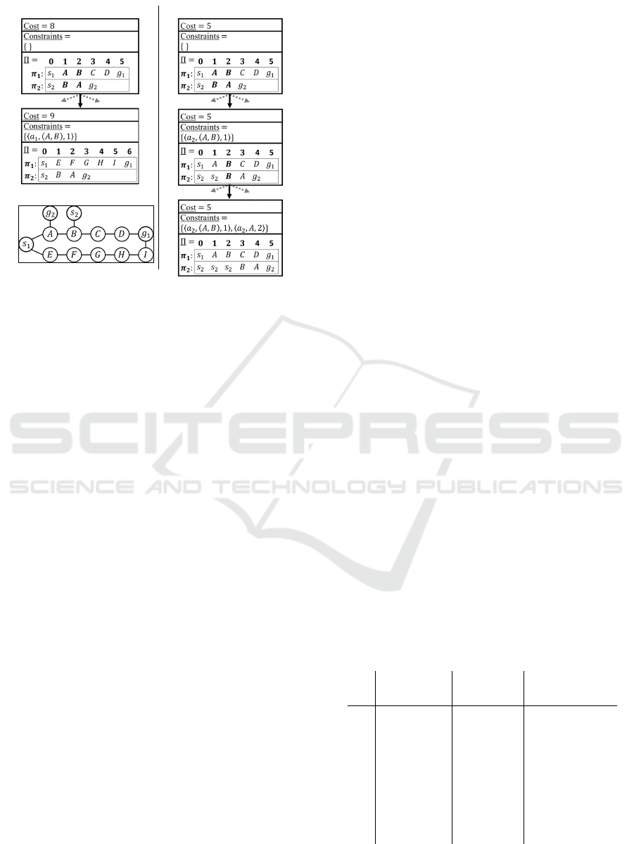
Figure 2CBS’s CTs for SOC (left) and MKS

(right). presents partial CTs for minimizing sum

of costs (left) and makespan (right) created when

CBS is executed on the problem instance shown

in Figure 1Example of SOC and MKS optimal

solutions.. The ﬁgure only presents the short-

est branches of the CTs leading to optimal solu-

tions. Here, C

SOC

(Root) = 8, C

SOC

(Π

SOC

) = 9, and

SOC

(Π

MSK

) = 10. Thus, ∆

SOC

= 1 and ∆

MSK

= 2,

corresponding to the depths of the optimal solutions.

While the lower bound on the depth of the op-

timal sum of costs is lower than that of the optimal

makespan, it may not always be the case that the op-

timal makespan solution is deeper in the CT than the

optimal sum of costs solution; it depends on the paths

the low-level solver returns, e.g., the low-level solver

It is shown (Boyarski et al., 2015) that resolving

conﬂicts in this order (cardinal, semi-cardinal, and non-

cardinal) often results in fewer CT node expansions.

ICAART 2024 - 16th International Conference on Agents and Artiﬁcial Intelligence

SOC

Makespan

Figure 1

Figure 2: CBS’s CTs for SOC (left) and MKS (right).

may return conﬂicting paths with non-cardinal con-

ﬂicts. Then the depth of the optimal solution may be

higher. Moreover, for CBS, some problem instances

are easier for sum of costs and some for makespan.

Figure 3Example of problem instances where

CBS performs better for SOC (left) and MKS (right).

presents two problem instances and their correspond-

ing CTs, where each CT node shows the sum of costs

and makespan of its plan. On the left instance, after

the conﬂict of the root is resolved, the sum of costs

and makespan increase in the left child CT node, and

only the sum of costs increases in the right one. As

the left node contains a conﬂict-free plan and the sum

of costs is equal for both nodes, an optimal sum of

costs solution is found, and the search can stop. How-

ever, to ﬁnd the optimal makespan solution, the right

node must be explored, as the makespan of that node

is lower. On the right instance, after the conﬂict of

the root is resolved, only the sum of costs in the left

CT node increases. Here, the optimal makespan solu-

tion is found in the left node, as both nodes have the

same makespan. However, to ﬁnd the optimal SOC

solution, the right node must be explored. Therefore,

the left instance is easier for ﬁnding the optimal sum

of costs solution and the right one is easier for ﬁnding

the optimal makespan solution.

While there are instances easier for either sum of

costs or for makespan, CBS still often performs bet-

ter for sum of costs. When resolving a conﬂict in

CBS, the sum of costs and makespan in the two child

CT nodes may either remain the same as their par-

ent or increase. Increasing the cost in the child nodes

usually reduces the size of the CT, as one of these

branches may not be explored, e.g., if the cost exceeds

the cost of the optimal solution. When the makespan

increases, the sum of costs always also increases, e.g.,

the left node of the left instance in Figure 3Example

of problem instances where CBS performs better for

SOC (left) and MKS (right).. However, when the sum

of costs increases, the makespan may not always in-

crease as well, e.g., the left node of the right instance.

Therefore, we conjecture that this also gives an ad-

vantage to sum of costs in CBS.

In the tiny maps (form size 8 by 8 to 24 by 24),

CBS performed slightly better for makespan than for

sum of costs. We conjecture that the reason is that

such maps are more crowded, the paths of the agents

are relatively short, and there is more than a single

agent inﬂuencing the makespan, i.e., multiple agents

have the longest path. Therefore, the makespan in-

creases more often in these maps when CBS resolves

a conﬂict between two agents.

Reduction to SAT. Both makespan and the sum of

costs optimizations pose speciﬁc challenges, which

we explain using the average number of variables in

instances solved by both the makespan optimal model

and iterative sum of costs optimal model shown in

Table 2Average number of variables (in thousands)

entering the SAT solver using the makespan optimal

model and the iterative sum of costs optimal model.

From left to right, the number of variables of the

last call, the number of times the SAT solver was in-

voked, and the cumulative number of variables across

all solver calls are listed.. Of course, other factors that

are hard to measure may play a role in performance in

the case of reduction-based solving, however, as we

show, the number of variables may provide an expla-

nation.

Table 2: Average number of variables (in thousands) enter-

ing the SAT solver using the makespan optimal model and

the iterative sum of costs optimal model. From left to right,

the number of variables of the last call, the number of times

the SAT solver was invoked, and the cumulative number of

variables across all solver calls are listed.

vars last call solver calls vars cumulative

mks soc mks soc mks soc

8 6 12 1,0 5,4 6 158

16 140 76 1,0 5,8 140 748

24 454 127 1,0 5,0 454 1269

32 1439 144 1,0 4,2 1439 1143

40 1685 130 1,0 4,5 1685 1183

48 1498 67 1,0 2,7 1498 451

56 1475 60 1,0 2,7 1475 382

64 1239 18 1,0 1,8 1239 53

The number of variables modeling the movement

Which Objective Function is Solved Faster in Multi-Agent Pathﬁnding? It Depends

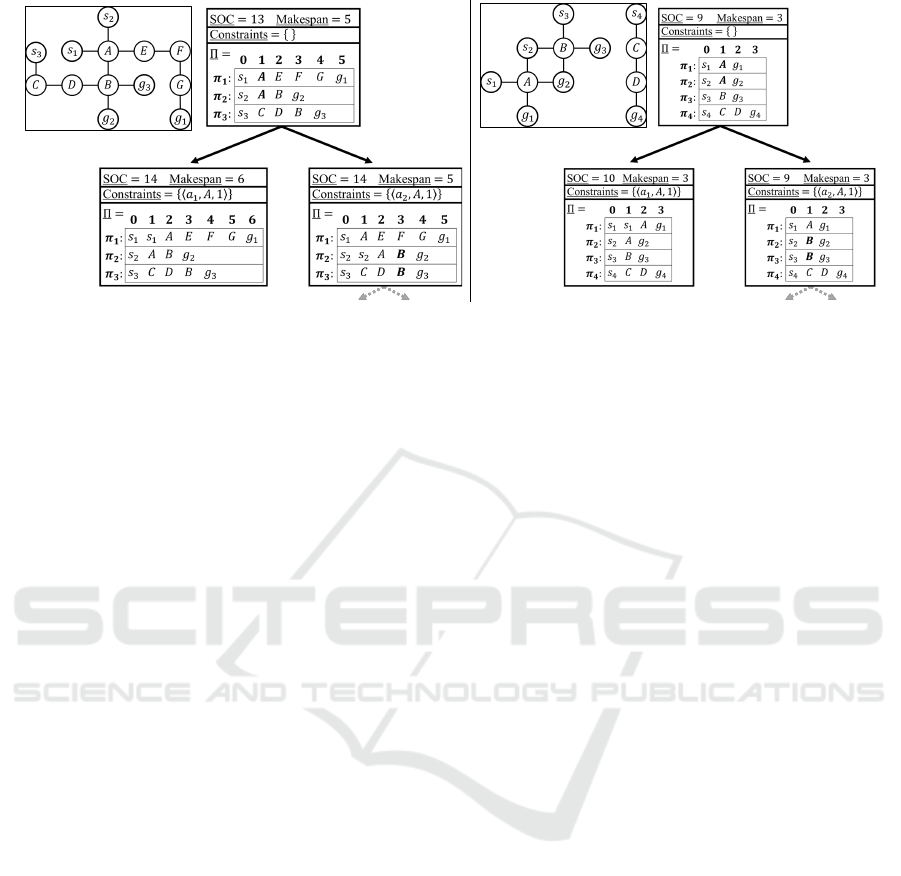
Figure 3: Example of problem instances where CBS performs better for SOC (left) and MKS (right).

of the agents depends on the number of agents |A|,

number of vertices |V |, and number of timesteps T .

Increasing |V | (i.e., increasing map size) increases

also T as the start and goal placement is random, it

is more likely that the start-goal distance is greater. In

the makespan optimization, there is a global time limit

T for all agents. This means that if the start-goal dis-

tance of agent a

is much lower than T , a

has enough

time and freedom to move around the map. For this

movement, variables have to be created and the un-

derlying solver has to assign them in compliance with

the constraints. These variables may be unnecessary

for ﬁnding the solution, however, to ensure that the

found solution is optimal, they have to be included.

The increase in the number of variables with the size

of the map can be seen in Table 2Average number of

variables (in thousands) entering the SAT solver using

the makespan optimal model and the iterative sum of

costs optimal model. From left to right, the number

of variables of the last call, the number of times the

SAT solver was invoked, and the cumulative number

of variables across all solver calls are listed.. The fact

that the number of variables decreases for map sizes

40 by 40 and onward is caused by both solvers not

being able to solve instances with a high number of

agents. On the other hand, as T is usually dictated

by a single agent with a large start-goal distance, T

is rarely increased as all conﬂicts are solved without

disturbing the critical agent. Again, this can be seen

in Table 2Average number of variables (in thousands)

entering the SAT solver using the makespan optimal

model and the iterative sum of costs optimal model.

From left to right, the number of variables of the

last call, the number of times the SAT solver was in-

voked, and the cumulative number of variables across

all solver calls are listed. in the number of solver calls,

which indicates how many times the bound on the cost

was increased.

In the sum of costs optimization, each agent has

a separate time limit T

. This means that the move-

ment of the agents is much more restricted and the

number of variables is lowered. On the other hand,

a numeric constraint “at most K” is introduced which

causes an overhead in terms of the number of vari-

ables. Table 2Average number of variables (in thou-

sands) entering the SAT solver using the makespan

optimal model and the iterative sum of costs optimal

model. From left to right, the number of variables

of the last call, the number of times the SAT solver

was invoked, and the cumulative number of variables

across all solver calls are listed. shows that the over-

head over the makespan model is most prominent in

the smallest maps. As the size of the map increases,

the makespan model overtakes the sum of costs model

due to the behavior explained above. Since the sum

of costs model poses a larger restriction on the move-

ment, the collisions among agents must be often re-

solved by increasing the cost function, meaning a new

call to the underlying solver (shown in Table 2Aver-

age number of variables (in thousands) entering the

SAT solver using the makespan optimal model and

the iterative sum of costs optimal model. From left

to right, the number of variables of the last call, the

number of times the SAT solver was invoked, and the

cumulative number of variables across all solver calls

are listed.). Since there are multiple solver calls, we

also present a cumulative number of variables across

all of the calls. These numbers more closely corre-

spond to the results in Table 1The number of solved

instances. The results are split based on the used cost

function and based on the size of the instance grid

graph. For each solver and map size, the most num-

ber of solved instances is highlighted.. Again, the fact

that the number of variables decreases for map sizes

40 by 40 and onward is caused by both solvers not

being able to solve instances with many agents.

Our results in Table 1The number of solved in-

stances. The results are split based on the used cost

ICAART 2024 - 16th International Conference on Agents and Artiﬁcial Intelligence

function and based on the size of the instance grid

graph. For each solver and map size, the most number

of solved instances is highlighted. also provide an in-

sight into the two different sum of costs optimal mod-

els – iterative and jump. In (Bart

ak and Svancara,

2019), the latter showed to outperform the former.

In our experiments, the iterative model always per-

formed better. The experiments in the original pub-

lication of the jump model were performed only on

small instances of sizes 8 by 8 up to 16 by 16, where

the model also performed the best in our experiments.

On these maps, the model can indeed outperform the

iterative model with improved implementation. As

stated, our implementation consists of hand-crafted

translation to SAT, while in the original paper, Picat

language is used (Zhou et al., 2015) to automatically

translate constraints to SAT and to minimize the sum

of costs. We suspect that the built-in libraries for min-

imization perform better than rebuilding the formula

from scratch with a different bound on the sum of

costs.

The jump model behaves differently as compared

to the iterative one. The number of solved instances

tend to decrease with the increase in map size for the

jump model, while the iterative model has a peak at

size 40 by 40. This is to be expected since the ﬁrst

step of the jump model is to ﬁnd the makespan optimal

solution and we showed that for the larger maps, it is

harder to ﬁnd the makespan optimal solution than the

sum of costs optimal solution. On the other hand, the

numerical constraints are still present and, as shown,

introduce a signiﬁcant overhead for the smaller maps.

In a sense, the jump model combines the hardest parts

of both optimizations.

On the other hand, the jump model performs fewer

solver calls to ﬁnd the appropriate k. The model may

be improved by ﬁnding a suboptimal solution ﬁrst (in-

stead of a makespan optimal one) to set the k.

Reduction to ASP. The results for the reduction to

ASP are similar to the ones for SAT. In Table 3Av-

erage number of variables, solve calls, and reachable

positions per instance for each cost function. Num-

bers for variables and positions are in thousands and

the number of variables is accumulated over all solve

calls., we see that the cumulative number of Boolean

variables follows a similar trend to that of SAT. How-

ever, the numbers are not directly comparable be-

cause they depend on the number of solved instances

and the ASP-based reduction solves slightly more in-

stances. The table also reports the number of reach-

able positions. We observe that this number is propor-

tional to the number of variables, which is to be ex-

pected because they directly inﬂuence the size of the

ground instances (the internal representation of the

encoding, closely related to a SAT formula, the solver

is working on). We observe that for the makespan ob-

jective, reachable positions increase for larger maps

but there is a drop for the largest maps. This can be

explained by the smaller number of instances solved

for larger maps; we can only solve for a low number

of agents. This behavior is even more pronounced for

the sum of costs objective. Furthermore, we observe

that there is a much higher number of solve calls for

smaller instances in this setting. This shows that we

can solve instances with more agents here. For larger

maps, the number of solve calls drops due to time-

outs coupled with a decrease in reachable positions.

This shows that the reachability optimization is espe-

cially effective for the sum of costs objective where

the shortest distances between start and goal vertices

are taken into account for each agent as opposed to

the makespan objective where all agents move within

the same ﬁxed horizon. Hence, we observe a much

smaller number of reachable positions and a larger

number of solved instances for the sum of costs ob-

jective as compared to the makespan objective.

Table 1The number of solved instances. The re-

sults are split based on the used cost function and

based on the size of the instance grid graph. For each

solver and map size, the most number of solved in-

stances is highlighted. shows that the jump model for

ASP performs worse than the iterative model. As dis-

cussed in the previous section, this can be improved

by changing the way the initial plan is computed. Fur-

thermore, we used the default conﬁguration of the

ASP solver in the benchmarks. We suspect that the

jump model would be faster than the iterative model

(at least for the smaller instances) if an alternative al-

gorithm for optimization is chosen, such as optimiza-

tion based on unsatisﬁable cores (Andres et al., 2012).

Finally, we comment on the difference in the num-

ber of solved instances between the SAT- and ASP-

based reductions. The instantiation of rules in the

ASP encoding is linear in the number of agents, while

for the reduction to SAT, the number of clauses for

conﬂicts is quadratic in the number of agents. Reduc-

ing the number of rule instances/clauses often has a

big impact on solving. We note that further size re-

ductions for the SAT model are possible as well.

7 CONCLUSION

We compared the behavior of the search-based al-

gorithm CBS and the reduction-based approaches

while optimizing MAPF under two cost functions –

makespan and sum of costs. We empirically showed

Which Objective Function is Solved Faster in Multi-Agent Pathﬁnding? It Depends

Table 3: Average number of variables, solve calls, and

reachable positions per instance for each cost function.

Numbers for variables and positions are in thousands and

the number of variables is accumulated over all solve calls.

vars cumulative solver calls reach pos

mks soc mks soc mks soc

8 12 264 1,0 7,0 2 67

16 189 436 1,0 5,3 28 119

24 692 699 1,0 5,1 102 196

32 2336 447 1,0 3,4 342 111

40 2900 273 1,0 2,7 426 60

48 2815 91 1,0 1,8 424 14

56 2646 180 1,0 2,3 396 37

64 1488 12 1,0 1,1 216 0,5

that on small-size maps, it is easier for both ap-

proaches to solve the makespan optimization, while

on larger maps, it is easier to solve the sum of costs

optimization. This is counter-intuitive since both of

the solving approaches were ﬁrst conceived for differ-

ent cost functions – search-based for the sum of costs

and reduction-based for makespan.

We provided insights into the phenomenon. For

CBS, the lower depth of the optimal makespan so-

lution is larger than or equal to that of the optimal

sum of costs solution, which may require more node

expansions when minimizing makespan. Moreover,

when the makespan increases at a child node due to

conﬂict resolution, the sum of costs also increases, but

not vice versa. Increasing that cost often reduces the

size of the CBS tree. Therefore, this also gives an ad-

vantage to the sum of costs. For the reduction-based

approaches, solving for sum of costs introduces over-

head for the numerical constraints. This overhead is

outweighed on larger maps by the freedom of move-

ment of the agents with less restricted paths. This

freedom is modeled by a large number of variables

that overwhelm the underlying solver.

We also compared our results with three previous

studies (Surynek et al., 2016b; Bart

ak and Svancara,

2019; G

omez et al., 2021) and showed that our results

are different from theirs due to the small-scale experi-

ments they used. On smaller maps, we observed sim-

ilar behavior as was reported in the studies, however,

on larger maps, the behavior diverged.

Based on our work, we propose open questions for

future work. The CBS algorithm may be improved for

makespan. When ﬁnding a new single-agent path, this

path does not have to be the shortest possible, if the

makespan is dictated by a path of a different agent.

This may reduce the number of future conﬂicts.

Furthermore, the jumping model may be improved

by changing the approach to ﬁnding the initial solu-

tion, as ﬁnding a makespan optimal solution ﬁrst and

then creating the numerical constraints combines the

hardest parts of both cost functions.

ACKNOWLEDGEMENTS

This work was funded by DFG grant SCHA 550/15,

by project 23-05104S of the Czech Science Founda-

tion, and by Charles University project 24/SCI/008.

REFERENCES

Alonso-Mora, J., Breitenmoser, A., Ruﬂi, M., Beardsley,

P. A., and Siegwart, R. (2010). Optimal reciprocal col-

lision avoidance for multiple non-holonomic robots.

In DARS, pages 203–216.

Andres, B., Kaufmann, B., Matheis, O., and Schaub, T.

(2012). Unsatisﬁability-based optimization in clasp.

In ICLP, pages 211–221.

As’in Ach’a, R. J., L

opez, R., Hagedorn, S., and Baier, J. A.

(2021). A new boolean encoding for MAPF and its

performance with ASP and maxsat solvers. In SoCS,

pages 11–19.

Bart

ak, R. and Svancara, J. (2019). On sat-based ap-

proaches for multi-agent path ﬁnding with the sum-

of-costs objective. In SoCS, pages 10–17.

Bennewitz, M., Burgard, W., and Thrun, S. (2002). Find-

ing and optimizing solvable priority schemes for de-

coupled path planning techniques for teams of mobile

robots. Robotics Auton. Syst., 41(2-3):89–99.

Biere, A., Fazekas, K., Fleury, M., and Heisinger, M.

(2020). CaDiCaL, Kissat, Paracooba, Plingeling and

Treengeling entering the SAT Competition 2020. In

Proceedings of the SAT Competition 2020 – Solver

and Benchmark Descriptions, pages 51–53.

Boyarski, E., Felner, A., Bodic, P. L., Harabor, D. D.,

Stuckey, P. J., and Koenig, S. (2021). f-aware conﬂict

prioritization & improved heuristics for conﬂict-based

search. In AAAI, pages 12241–12248.

Boyarski, E., Felner, A., Stern, R., Sharon, G., Tolpin,

D., Betzalel, O., and Shimony, S. E. (2015). ICBS:

improved conﬂict-based search algorithm for multi-

agent pathﬁnding. In IJCAI, pages 740–746.

Dresner, K. M. and Stone, P. (2008). A multiagent

approach to autonomous intersection management.

JAIR, 31:591–656.

Felner, A., Li, J., Boyarski, E., Ma, H., Cohen, L., Kumar,

T. K. S., and Koenig, S. (2018). Adding heuristics to

conﬂict-based search for multi-agent path ﬁnding. In

ICAPS, pages 83–87.

Gebser, M., Harrison, A., Kaminski, R., Lifschitz, V., and

Schaub, T. (2015). Abstract Gringo. Theory and Prac-

tice of Logic Programming, 15(4-5):449–463.

omez, R. N., Hern

andez, C., and Baier, J. A. (2021). A

compact answer set programming encoding of multi-

agent pathﬁnding. IEEE Access, 9:26886–26901.

ICAART 2024 - 16th International Conference on Agents and Artiﬁcial Intelligence

Hart, P., Nilsson, N. J., and Raphael, B. (1968). A formal

basis for the heuristic determination of minimum cost

paths. IEEE Transactions on Systems Science and Cy-

bernetics, 4:100–107.

Hus

ar, M., Svancara, J., Obermeier, P., Bart

ak, R., and

Schaub, T. (2022). Reduction-based solving of multi-

agent pathﬁnding on large maps using graph pruning.

In AAMAS, pages 624–632.

Kaminski, R., Romero, J., Schaub, T., and Wanko, P.

(2020). How to build your own asp-based system?!

CoRR, abs/2008.06692.

Li, J., Felner, A., Boyarski, E., Ma, H., and Koenig, S.

(2019). Improved heuristics for multi-agent path ﬁnd-

ing with conﬂict-based search. In IJCAI, pages 442–

449.

Ma, H., Li, J., Kumar, T., and Koenig, S. (2017). Lifelong

multi-agent path ﬁnding for online pickup and deliv-

ery tasks. In AAMAS, pages 837–845.

Nguyen, V., Obermeier, P., Son, T. C., Schaub, T., and

Yeoh, W. (2017). Generalized target assignment and

path ﬁnding using answer set programming. In IJCAI,

pages 1216–1223.

Philipp, T. and Steinke, P. (2015). Pblib – a library for en-

coding pseudo-boolean constraints into cnf. In Theory

and Applications of Satisﬁability Testing – SAT 2015,

volume 9340 of Lecture Notes in Computer Science,

pages 9–16. Springer International Publishing.

Sartoretti, G., Kerr, J., Shi, Y., Wagner, G., Kumar, T.

K. S., Koenig, S., and Choset, H. (2019). PRI-

MAL: pathﬁnding via reinforcement and imitation

multi-agent learning. IEEE Robotics Autom. Lett.,

4(3):2378–2385.

Sharon, G., Stern, R., Felner, A., and Sturtevant, N. R.

(2015). Conﬂict-based search for optimal multi-agent

pathﬁnding. Artiﬁcial Intelligence, 219:40–66.

Silver, D. (2005). Cooperative pathﬁnding. In AIIDE, pages

117–122.

Stern, R., Sturtevant, N. R., Felner, A., Koenig, S., Ma, H.,

Walker, T. T., Li, J., Atzmon, D., Cohen, L., Kumar,

T. K. S., Bart

ak, R., and Boyarski, E. (2019). Multi-

agent pathﬁnding: Deﬁnitions, variants, and bench-

marks. In SoCS, pages 151–159.

Surynek, P. (2010). An optimization variant of multi-robot

path planning is intractable. In AAAI, pages 1261–

1263.

Surynek, P. (2012). A sat-based approach to cooperative

path-ﬁnding using all-different constraints. In SoCS.

Surynek, P. (2017). Time-expanded graph-based proposi-

tional encodings for makespan-optimal solving of co-

operative path ﬁnding problems. Ann. Math. Artif. In-

tell., 81(3-4):329–375.

Surynek, P., Felner, A., Stern, R., and Boyarski, E. (2016a).

Efﬁcient SAT approach to multi-agent path ﬁnding un-

der the sum of costs objective. In ECAI, pages 810–

818.

Surynek, P., Felner, A., Stern, R., and Boyarski, E. (2016b).

An empirical comparison of the hardness of multi-

agent path ﬁnding under the makespan and the sum

of costs objectives. In SoCS, pages 145–147.

Yu, J. and LaValle, S. M. (2012). Multi-agent path planning

and network ﬂow. In WAFR, pages 157–173.

Yu, J. and LaValle, S. M. (2013). Structure and intractability

of optimal multi-robot path planning on graphs. In

AAAI, pages 1444–1449.

Zhou, N. and Bart

ak, R. (2017). Efﬁcient declarative solu-

tions in picat for optimal multi-agent pathﬁnding. In

ICLP, pages 11:1–11:2.

Zhou, N., Kjellerstrand, H., and Fruhman, J. (2015). Con-

straint Solving and Planning with Picat. Springer

Briefs in Intelligent Systems. Springer.

Which Objective Function is Solved Faster in Multi-Agent Pathﬁnding? It Depends