A Study of the Images Classification on the CIFAR10 Dataset Based

on CNNs

Xuanyi Shen

School of Electronic and Information Engineering, Tongji University, Shanghai, China

Keywords: Convolutional Neural Networks, Image Classification and Identification, Cifar10, Machine Learning,

Optimization Algorithm.

Abstract: Realizing the purpose of identifying and classifying the images relies on machine learning and deep learning

methods. It is about building the model and training and testing it. The model calculates the data in the layers

and nerve cells inside and creates the most suitable links and relationships between the images and labels.

According to the results summary and evaluation indicators, the parameters are adjusted to get the most ideal

optimization algorithm, with the highest accuracy and efficiency and least loss. In this paper, a Convolutional

Neural Network (CNN) model is built and used to work on the Cifar10 dataset. Its mission is to successfully

divide the pictures in the testing set into 10 classes, after being trained by the pictures in the training set and

find the most workable algorithm after adjusting to see how well CNNs indeed do while operating the

visualizing materials. About the results, it is easy to tell that this method is of great success. The accuracy of

it reaches as high as 87.29% while testing, with only the loss of 0.39. Additionally, the efficiency of it is also

high enough. To make the conclusion more scientific, this model is compared by the Naïve Bayes model, and

the CNN performs apparently rather better than the traditional ones when facing such complex data. Thus,

there is the conclusion that the CNN methods are quite capable of work of identifying and classifying the

images.

1 INTRODUCTION

The idea of the whole program and this paper

undoubtedly comes from today’s everyday life. As the

science and technology developing, it is obvious that

an increasing number of people become really into the

internet. Paying more attention to the websites and

software, it will be noticed that there are

miscellaneous user authentication applications when

browsing certain websites, including Steam, Google

and so on. So, the technology of images identifying

and classification is getting more and more attention

due to its wide application. Thus, the overarching goal

of this project is to build the most expeditious and

stable algorithm that can sifts out those irrelevant

figures and identify the correct type of photos.

In this study, the CNN models of the machine

learning methods, which are being well developed and

hot for computer science research workers across the

world to conduct some studies on them in recent

period, are used and studied to realize the purpose.

And here is its basic principle. Since the images

contain mountains of complex information, such as

pixels and colors, a large number of pictures from the

dataset, which have already been classified, are sent to

the machines and models together with their labels as

training sets to provide enough information for them.

Then these inputs are collected, preprocessed,

calculated, analyzed and remembered through the

layers of the models and the complicated math

formulas of them, which in this model works in the

way that seeing the pictures as matrixes and using the

operating formula developed based on convolution.

In this way, the model finds out the links between

input images and the aiming output values, the

classification labels. After all these training, a set of

different pictures is used as testing sets to see the

function of the model, with the results summary and

evaluation indicators displayed. And the further

adjustments are carried out in order to better the

accuracy and accelerate the learning path, until the

ideal model is built up.

About this paper, it is organized in the following

construction. After this introduction part, the next

section presents related work on the development and

current situation of the machine learning and CNN

114

Shen, X.

A Study of the Images Classiﬁcation on the CIFAR10 Dataset Based on CNNs.

DOI: 10.5220/0012798800003885

Paper published under CC license (CC BY-NC-ND 4.0)

In Proceedings of the 1st International Conference on Data Analysis and Machine Learning (DAML 2023), pages 114-118

ISBN: 978-989-758-705-4

models. Then the whole study is discussed specifically

next, including its methods, principles, used dataset,

results and current analysis on it. And the last part,

based on the entire paper, the conclusions are made

and some ideas of the future work directions and

suggested.

2 RELATED WORK

As the technology developing, machine learning and

deep learning have gradually developed for a quite

long period. They are based on different math

principles and formulas dealing with the numeric

input dataset. And their realization relies on the

optimization algorithms of different parameters. So, it

is noticeable that the algorithms are playing very vital

roles and various studies have been conducted to

researching on these.

At first, the traditional methods of machine

learning are only capable of operating on the data that

is not really complicated, such as Naïve Bayes and

SVM method. Their ways of operating the data are

more like stacking all the input data into its formulas

straightly and raising the accuracy through adjusting

the parameters. However, as the rapid development of

the times, especially when they begin to facing the

images data, they apparently fail to do the job

successfully. Thus, the more intelligent deep learning

methods are invented.

So, when here comes the deep learning, the ability

for the machines to operate those complex data

samples. The CNNs get the idea from the

neuroscience and the thought of nerve cell and layers

is insert in the method to enable it to have the ability

to create the links, which is obviously different with

the stiffly applying formulas that the traditional

methods do. Although the fundamental idea to build

this model also comes from the arithmetical operation

in math just like traditional ones, the reason why it

differs from other old ones is that it has the ability to

make links between the classes and labels and process

multiply every pictures in training batch.

Thus, the CNNs are now involved in almost every

aspect that the image identification is used, such as,

predicating the weather according to the satellite cloud

picture, the classification used in website to apart

human beings and AIs and the Face ID of the phones

etc. And it is always on a rapid developing path, with

many new architectures coming out with rather short

interval, like the VGG16 coming out 10 years ago and

the ResNet model 8 years ago (Laszlo and Nagy 2020

& Xie et al 2019). And there are various operating

methods like backpropagation, new gradient descents,

deep Residual learning and global average pooling

(Jing et al 2023 &

Hassan et al 2023).

Thus, this paper builds and tests the Convolutional

Neural Network models on a large dataset and

compares its outcomes with those of traditional

methods such as Naïve Bayes methods, aiming to see

its accuracy and efficiency.

3 METHDOLOGY

3.1 Building the Model

While using the Convolutional Neural Networks to

realize the image identification and classification, the

first step of the process is to load labeled images from

the CIFAR-10 dataset and to preprocess the data. The

data has already been segmented into training sets and

testing sets that can be straight insert in the program

without pre-processing. So, firstly, the pixel value of

each picture is scaled to between 0 and 1 by being

divided by 255.0. While the target variable, which are

the class names and labels of the images, are transform

into One-Hot Encoding.

Then, it is time to build the model, and this

program uses the Sequential model. In this model, the

convolution operation in the Convolutional Layers is

the core part of CNNs. In this program, the data are

inputted in the shape of (32,32,3). And by convolving

the images with the learnable kernels with the size of

(3,3), features are extracted from the image. Each

filter in kernels detects different local features, such as

edges or textures. And the formula of the convolution

in this program is S(i,j)=(I∗K)(i,j)=m∑n∑

I(i−m,j−n)⋅K(m,n), with S and I referring to the pixel

value of the output images and input images and K

referring to the kernels (Raheer and Humera 2019).

Also, in these layers, a non-linear activation

function, which is ReLU in this program, is applied to

introduce non-linearity and enhance the expressive

power of the model. The formula is

ReLU(x)=max(0,x), where x represents the input. The

convolution operation and the activation function are

all realized by Conv2D function in this program in

Python. And whenever a Conv2D layer is finished, the

BatchNormalization function is used to normalize the

features in the former layers to make the training

easier, faster and more stable (Biniz and Ayachi 2021).

Then, in the Pooling Layers, the pooling jobs are

done by max pooling in the size of (2,2), whose

formulas is MaxPooling2D(i,j,c)=m,nmax

(x(i+m),(j+n),c), with(i,j,c) referring the places in the

output images and x referring the amount in polling

(Park et al 2022). Through these, pooling operations

A Study of the Images Classiﬁcation on the CIFAR10 Dataset Based on CNNs

115

can help decrease the size of the feature maps while

preserving those features that are relatively more

important.

Then in order to raise the accuracy of the program

and realize more ideal outcomes, Convolutional

Layers and Pooling Layers with different filters

parameters, 32 64 128 individually, are used

alternately and circularly for a few times.

After all the steps above, the next layer is the

Flatten Layer. The aim of inserting it is to reshape the

outputs from the previous layers, which are multi-

dimensional arrays, into a single long vector. So that

they can be fed into subsequent fully connected layers

for further processing, because these layers can only

accept this kind of one-dimensional input.

Then here comes the Fully Connected Layers in

the model. These layers connect all the features of the

data. In this program, the two Dense functions with

different parameters, which are 128 and 10 in this

program and refer to the number of neurons in this

layer, are used as Fully Connected Layers to do the

linking job between the former layers that has been

built before and the current ones that are being built.

And the task for them in to successful put the neurons

from the two different layers together and create links

to enable them to work as an entirety.

Additionally, the activations of the two layers

above are also different, which are relu and softmax.

What is more, nearly after every layer, a Dropout

function with the parameter of 0.25 is used in this

program to prevent the model from overfitting, so that

the accuracy and the stability of the model can be

guaranteed. After these steps and layers, the model is

finally built.

3.2 Training and Testing

So, the next part is to train and test the model that has

been built. In this part, the training set is used to train

the model, to enable it to identify the pictures and do

the classification. The model is evaluated on the

testing set to measure its results, which are displayed

by printing the summary and the confusion matrix,

and its many performance metrics, including

accuracy, recall, loss and precision etc. And this can

help to judge and prediction how the model performs

when operating on a new set of data.

Then, the next job is to keep adjusting all the

parameters in the program and adding or decreasing

the number of layers according to the performance and

prediction, until the best and most accurate outcomes

are got and ready for analysis and conclusion.

4 RESULT

In this program, the dataset that is used is the widely-

used CIFAR-10dataset.

The CIFAR-10 dataset is got from the Kaggle and

can be imported in the program straightly from the

keras of tensorflow. The CIFAR-10 dataset is made up

of 60 thousand images in 10 different themes with

various colors, with exactly 6000 ones in every single

class, and each picture contains 32*32 pixels. The ten

classes are in a fixed order while using for the better

convenience, which is 'Airplane', 'Automobile', 'Bird',

'Cat', 'Deer', 'Dog', 'Frog', 'Horse', 'Ship', 'Truck', and

it may be mentioned in the following paper by using

the number zero to nine. And every picture can be

visible on the Kaggle or by coding (Iqbal and Qureshi

2023).

Using this dataset has its own convenience. In this

dataset, the images have already been divided into the

training and testing groups. 50 thousand training

pictures and 10 thousand test pictures have been pre-

prepared already in this dataset. What is more, it is

divided into five training lots and a test lot, each is

made up of 10 thousand images, which appear in a

stochastic combination every time being used.

Considering from the aspect of the classes, each one

of the ten classes provide one thousand images, which

are randomly selected as said before, to form the final

test batch. Meanwhile, the rest of the pictures in each

class are undoubtedly contained in those five training

batches in a random formed order that no one knows.

Also, unlike the testing one, the training lot have on

force on that the images from each class must be of

the same number. That means that there may not be

exactly 500 pictures in a single batch, but there are

undoubtedly exactly 5000 pictures in the whole

training part, the five lots.

First, the model should be evaluated according to

its summary of results and all of its evaluation

indicators. Taking all into consideration, the model is

quite successful. The analysis can be based on the

classification report of the testing results after the

attempting of each time.

From all the information in the Table 1, it can be

found out that all the evaluation indicators, the

precision, the recall and the f1-score, of all the ten

classes are totally of a very high level. There is only

one class having the least precision of 77%, while all

the other ones are above 80%, with some of them are

so high that they reach or even surpass ninety

percents. Also, it is easy to find out that except the

class 3, all the recalls and f1-scores are all at such a

high area that they are individually over or close to

80% and 85%. The least f1-score also occurs in the

DAML 2023 - International Conference on Data Analysis and Machine Learning

116

class 3. From all these, it can be reasonably speculated

that the model performs relatively worst in class 3. But

all this can be concluded into the overall high accuracy

of 87%. So, this report shows that this model of using

the CNN method to identify and classify the images

performs rather well and fits in the CIFAR-10 dataset

quite greatly.

Table 1: Classification Report.

Precision Recall F1-score

0 0.90 0.87 88%

1 0.94 0.96 95%

2 0.80 0.85 83%

3 0.85 0.67 75%

4 0.86 0.88 87%

5 0.88 0.77 82%

6 0.77 0.96 85%

7 0.92 0.92 92%

8 0.96 0.91 93%

9 0.89 0.94 92%

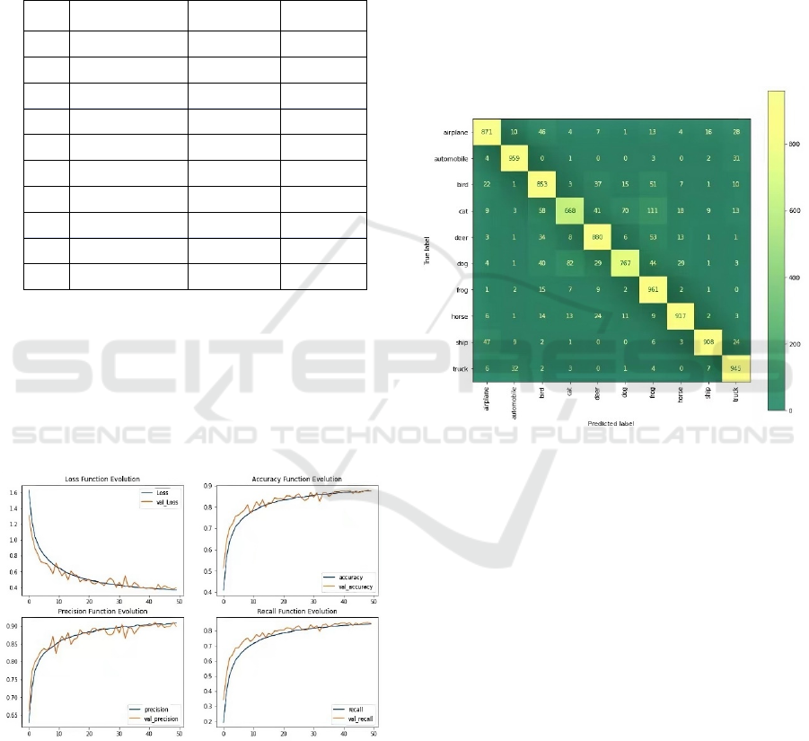
Additionally, beyond the information above, more

things can be found out from the Evolution Legend

Graphs. They are the curve graphs shows the changing

of the different parameters, including loss, accuracy,

precision and recall, during the training progresses,

whose rate can be somehow on behalf of the efficiency

of this model.

Figure 1: Evolution Legend Graphs (Photo/Picture credit:

Original).

From the graphs in Figure 1, the advantage and the

success of this model is more obvious. It is easy to

discover that the accuracy, precision and recall all

reach to a high and stable level rather fast during the

training, which is showed by the large slope in the

beginning of the graph., while the loss performs

exactly opposite. These shows that this CNN model

has a really good capability of learning on the

identification and classification of the pictures, at least

the pictures of the CIFAR10 dataset, which is just the

purpose of building it.

Additionally, the confusion matrix is used to have

further comparison and analysis, since that the

confusion matrix uses the variety and asymptote of the

shade of the colors to symbolize the number of every

situation. This enables the researchers to realize and

compare the results more intuitional and have more

meaning conclusions.

Figure 2: Confusion Matrix (Photo/Picture credit: Original).

From Figure 2, according to the obvious

distinguishment of the colors between yellow and

green, it is more visualized and easier to tell that how

well this CNN model performs while working on such

difficult pictures database. Except for the large

number of the right classified images, it can be found

that the model did worst on the ‘Cat’ and ‘Dog’

classes. And the reason for the weakness can be

assumed that this model performs not really well in

distinguishing cats and dogs and it may sometimes

identify the cats as frogs. And these are the current

problems that the model is facing now.

In searching for more conclusions and reach the

more helpful and in-depth outcomes, this model is

compared to a traditional machine learning model

based on the GaussianNB function of the Naïve

Bayesian method, with the data preprocessed by the

PCA (Chen et al 2018 & Zhang 2023). This is a

traditional classifier of operating the data and dividing

them into different classifications, according to the

A Study of the Images Classiﬁcation on the CIFAR10 Dataset Based on CNNs

117

simplified Bayes formular, which may be simplistic

while facing such difficult image data.

Table 2: Comparison.

Naïve Bayes CNN

Accuracy 35.25% 87.29%

recall 35.25% 84.97%

precision 35.47% 89.92%

According to TABLE II, the CNN has obviously

far higher three indicators than the Naïve Bayes. That

shows that when operating such complex data as

images, the CNN model performs rather better than

traditional ones, even still with great potential that

hasn’t been explored yet. The reason for the

distinction may be that the images data is too

complicate and it may contain nonlinear relationships

and high-dimensional feature space, which are all

great challenges for traditional models, such as Naïve

Bayes and SVM etc. But all those can be somehow

solved by CNN’s ability of deep feature learning,

which empowers CNNs to better capture hierarchical

patterns and structures within images.

5 CONCLUSION AND FUTURE

WORK

This study is research on building and using the CNN

models to train and test on the CIFAR-10 dataset and

comparing it with other traditional models. According

to the results, comparison and analysis that has been

done before, there are some current conclusions can

be made. The CNN model has a great capability of

recognizing, identifying and classifying the images. It

has a high accuracy on dividing them into different

classes and its speed of learning and training is rather

fast. Taking the traditional models into consideration,

the CNN models are better than them in nearly every

aspect. Thus, CNN is one of the most expeditious and

stable models that can be used to solve the image

recognition and classification problems.

For the future work, similar models with varying

parameters combination can be studied on the same or

even larger dataset to see if they can bring higher

accuracy and learning ability. Additionally, some

other operations can be studied and inserted into this

model, such as data processing ones, to better the

program to get higher accuracy and speed. So, the

future works based on this program can be brought out

from these aspects to build better models with higher

accuracy and efficiency.

REFERENCES

Laszlo C and A.M. Nagy, "Improving object recognition of

CNNs with multiple queries and HMMs,"

International Conference on Machine Vision (SPIE),

2020, pp. 2559393.

Q. Xie, K. Zhou and X. Fan, "A Scene Text Detection

Algorithm based on ResNet and Faster R-CNN,"

Proceedings of the 2019 International Conference on

Artificial Intelligence and Computer Science (AICS

2019), 2019, pp. 840-843.

R. Jing, R. Gao and M. Liu, et al, “A variable gradient

descent shape optimization method for transition tee

resistance reduction,” Building and Environment, vol.

244, no. 1, pp. 110735, 2023.

R. Hassan, M.M. Fraz, A. Rajput, et al, “Residual learning

with annularly convolutional neural networks for

classification and segmentation of 3D point clouds,”

Neurocomputing, vol. 526, no. 14, pp. 96-108, 2023.

Z. Raheer and S. Humera, “A study of the optimization

algorithms in deep learning,” in 2019 third

international conference on inventive systems and

control (ICISC), 2019, pp. 536-539.

M. Biniz, and R.E. Ayachi, “Recognition of Tifinagh

Characters Using Optimized Convolutional Neural

Network,” Sensing and Imaging, vol. 22, no. 28, pp.

109-118, 2021.

G.H. Park, J.H. Park and H.N. Kim, “Convolutional Neural

Network-Based Target Detector Using Maxpooling

and Hadamard Division Layers in FM-Band Passive

Coherent Location,” Journal of Electromagnetic

Engineering and Science, vol. 22, no. 1, pp. 21-27,

2022.

T. Iqbal, and S. Qureshi. "Reconstruction probability-based

anomaly detection using variational auto-

encoders," International Journal of Computers and

Applications, vol. 45, no. 3, pp. 231-237, 2023.

X. Chen, B. Fan, W. Yang, et al, “Air-Attack Weapon

Identification Model of Weighted Navie Bayes Based

on SOA,” Asia Pacific Institute of Science and

Engineering (APISE), in 2018 2nd International

Conference on Data Mining, Communications and

Information Technology (DMCIT), 2018, pp. 012054.

N. Zhang, Y. Zhong and S. Dian, “Rethinking unsupervised

texture defect detection using PCA,” Optics and

Lasers in Engineering, vol. 163, pp. 107470, 2023.

DAML 2023 - International Conference on Data Analysis and Machine Learning

118