A Comparison of the State-of-the-Art Evolutionary Algorithms with

Different Stopping Conditions

Jana Herzog

, Janez Brest

and Borko Bo

skovi

Faculty of Electrical Engineering and Computer Science,

University of Maribor, Koro

ska cesta 46, Maribor, Slovenia

Keywords:

Evolutionary Algorithms, Fixed-Budget Approach, Stopping Conditions.

Abstract:

This paper focuses on the comparison of the state-of-the-art algorithms and the inﬂuence of a stopping condi-

tion, the maximum number of function evaluations, on the optimization process. The main aim is to compare

the chosen state-of-the-art algorithms with different predetermined stopping conditions and observe if they are

comparable in reaching a certain quality of solution on a given set of benchmark functions. For this analysis,

the four most recent state-of-the-art evolutionary algorithms were chosen for comparison on the latest set of

benchmark functions. We utilized a ﬁxed-budget approach with different values of stopping conditions. Small

differences in the algorithms’ performances are observed and the obtained results are also statistically ana-

lyzed. Different values of the stopping conditions show different rankings of evolutionary algorithms without

the signiﬁcant difference. The possible reason for this is that their performances are very close.

1 INTRODUCTION

It is extremely demanding to improve an evolu-

tionary algorithm’s performance for a speciﬁc set

of benchmark functions. Various mechanisms can

be helpful in such tasks, for example mechanisms

such as population size reduction (Tanabe and Fuku-

naga, 2014), (Piotrowski et al., 2020), perturbation

techniques (Van Cuong et al., 2022), using multi-

ple mutation strategies (Zhu et al., 2023), multiple

crossover techniques (Bujok and Kolenovsky, 2022),

self-adaptive parameters (Brest et al., 2014) and re-

initialization mechanism (Meng et al., 2021). The

aim of these mechanisms is the same; to enhance and

reﬁne the algorithm’s performance to reach a better

quality of solutions, to increase the speed of con-

vergence, or to lower the runtime while considering

a ﬁxed-budget (Jansen, 2020) or a ﬁxed-target ap-

proach (Hansen et al., 2021).

With the ﬁxed target approach, we set a speciﬁc

value as a target value (quality of solution) and ob-

serve if it will be reached by a given algorithm. Here

we also observe the number of function evaluations or

runtime spent to reach the optimal or suboptimal tar-

https://orcid.org/0000-0001-5555-878X

https://orcid.org/0000-0001-5864-3533

https://orcid.org/0000-0002-7595-2845

get value. While, with the ﬁxed-budget approach, we

set a speciﬁc budget (number of function evaluations

or runtime) and observe the quality of the solution that

will be reached.

However, both approaches have some shortcom-

ings, for example with the ﬁxed-budget approach, the

algorithm is restricted to a certain number of func-

tion evaluations. This can hinder the algorithm’s abil-

ity to explore the search space fully and it can result

in solutions of suboptimal quality. Whereas for the

ﬁxed-target approach, a choice of targets may present

a challenge, since not every solver is able to reach the

wanted quality of solutions.

The main intention of every experiment is to reach

the optimal solution with the smallest possible num-

ber of function evaluations as possible, while also

observing the best quality of solutions. The maxi-

mum number of function evaluations or the budget

(in the ﬁxed-budget approach) is a common stop-

ping condition used in competitions, such as IEEE

Congress on Evolutionary Computation (CEC) Spe-

cial Sessions and Competitions on Real-Parameter

Single-Objective Optimization (A. W. Mohamed, A.

A. Hadi, A. K. Mohamed, P. Agrawal, A. Kumar,

P. N. Suganthan, 2020), (A. W. Mohamed, A. A.

Hadi, A. K. Mohamed, P. Agrawal, A. Kumar, P.

N. Suganthan, 2021). In the CEC competition, al-

most every year, a new set of benchmark functions

222

Herzog, J., Brest, J. and Boškovi

c, B.

A Comparison of the State-of-the-Art Evolutionary Algorithms with Different Stopping Conditions.

DOI: 10.5220/0012182200003595

In Proceedings of the 15th International Joint Conference on Computational Intelligence (IJCCI 2023), pages 222-229

ISBN: 978-989-758-674-3; ISSN: 2184-3236

is utilized to compare the newest proposed state-of-

the-art evolutionary algorithms under the same set

of conditions (A. W. Mohamed, A. A. Hadi, A. K.

Mohamed, P. Agrawal, A. Kumar, P. N. Suganthan,

2021). The problem occurs when some algorithms

are budget dependent (Tu

sar et al., 2017), mean-

ing that some of their parameters are set based on

the stopping condition maxFEs (maximum number of

function evaluations). Some of the evolutionary al-

gorithms use maxFEs as a control parameter in the

mechanism of the population size reduction. There,

it affects the population size and consequently inﬂu-

ences the optimization process. Examples of such

state-of-the-art algorithms are L-SHADE (Tanabe and

Fukunaga, 2014), iL-SHADE (Brest et al., 2016) and

MadDE (Biswas et al., 2021).

It is even more difﬁcult to predict algorithm’s per-

formance while using a different budget from the one

being used in the experiment of the given/cited pa-

per or competition (Hansen et al., 2021). Furthermore,

a programming language can play a signiﬁcant role

in determining the prevailing algorithm on a given

benchmark. This holds true in cases, when the ob-

served variable is runtime or speed (Herzog et al.,

2022), (Ravber et al., 2022).

The question which arises is following: how com-

parable are the state-of-the-art algorithms based on

different predetermined stopping conditions? Are

some of the state-of-the-art evolutionary algorithms

adapted for a certain stopping condition?

In this paper, it is shown how different predeter-

mined stopping conditions affect the chosen evolu-

tionary algorithms in reaching a certain quality of so-

lutions. For the purpose of this analysis, four state-

of-the-art algorithms were chosen: EA4eig (Bujok

and Kolenovsky, 2022), NL-SHADE-RSP (Biedrzy-

cki et al., 2022), NL-SHADE-LBC (Stanovov et al.,

2022), and S-LSHADE-DP (Van Cuong et al., 2022).

All four evolutionary algorithms were compared on

the CEC 2022 Benchmark functions. We present the

statistical analysis and describe how the ranking of

the chosen algorithms changes when a different maxi-

mum number of function evaluations is being applied.

We ran the algorithms with the original settings from

the competition (A. W. Mohamed, A. A. Hadi, A. K.

Mohamed, P. Agrawal, A. Kumar, P. N. Suganthan,

2021) and then we modiﬁed the maximum number of

function evaluations to see whether there are any dif-

ferences between the algorithms’ ranks or their per-

formances.

The paper is organized as follows. In Section 2,

the related work is described. In Section 3, the ex-

periment and analysis are provided. Section 4 ﬁnally

concludes our paper.

2 RELATED WORK

It is extremely difﬁcult to deduce, which algorithm

is the best for a chosen optimization problem. In this

section, we will present a few of the newer approaches

which tackle the stochastic algorithm’s analysis and

we will emphasize what they focus on.

The questions which occur in terms of the perfor-

mance analysis are for example the following, how

fast can an algorithm reach a wanted solution qual-

ity and with what budget this can be achieved (Bartz-

Beielstein et al., 2020). The answers are provided by

the ﬁxed-target or ﬁxed-budget approaches. One of

the most common measurements of evaluating an al-

gorithm is the number of function evaluations (NFEs).

For example, the aim of some methods is to achieve

the smallest number of function evaluations in reach-

ing the optimal solution. However, some of the anal-

yses focus more on the speed or runtime of the algo-

rithm (Herzog et al., 2022). The measurement of time

can be sensitive to some factors, such as the program-

ming language, hardware, or even of the workload of

the CPUs. This aspect makes algorithms more difﬁ-

cult to compare (Bartz-Beielstein et al., 2020).

However, all research is aimed towards establish-

ing a fair comparison of evolutionary algorithms and

choosing the best one for a given optimization prob-

lem. Furthermore, the analyses should be also aimed

towards choosing the best algorithm for real-world

problems (Bartz-Beielstein et al., 2020).

The anytime approach (Hansen, Nikolaus and

Auger, Anne and Brockhoff, Dimo and Tu

sar, Tea,

2022), argues that the appropriate measurement to

provide a quantitative and meaningful performance

assessment is the number of blackbox evaluations to

reach a predeﬁned target value. They call this mea-

sure the runtime of the algorithm. It is also budget-

free since the authors support the claim that bench-

marking for a single budget seems inefﬁcient. Fur-

thermore, it does not provide enough information

about the solver or the optimization problem. The

approach is able to assess the performance anytime.

The main focus is on using quantitative performance

measures on a ratio scale and runtime measurements.

It is no longer enough to choose only one algo-

rithm for a given set of benchmark functions (Wolpert

and Macready, 1997), but to choose the best algo-

rithm for each problem instance. This problem can

be mitigated by using the automated algorithm selec-

tion (Cenikj et al., 2022). This approach emphasizes

that different instances are best solved when different

algorithms are being used (Kerschke et al., 2019). Re-

searchers have been focusing mostly on the character-

istics of an algorithm, however the focus should also

A Comparison of the State-of-the-Art Evolutionary Algorithms with Different Stopping Conditions

223

be on the characteristics of an optimization problem.

In (Herzog et al., 2023), it is shown how to predict

a stopping condition for a speciﬁc optimization prob-

lem and stochastic solver with a certain probability.

The prediction model is based on the statistical distri-

bution of two variables (runtime and number of func-

tion evaluations). Based on the smaller dimensions

of an optimization problem and a chosen stochastic

solver, one is able to predict in what runtime or num-

ber of function evaluations a solution of wanted qual-

ity will be reached with any probability for larger di-

mensions.

An interest has been taken recently in exploratory

landscape analysis, which characterizes optimization

problem instances with numerical features, which de-

scribe different sides of the problem instances (Niko-

likj et al., 2022). The approaches changed also in

terms of not only choosing an algorithm suitable for a

benchmark but vice-versa. The SELECTOR (Cenikj

et al., 2022) approach focuses on selecting a represen-

tative set of benchmark functions to provide a repro-

ducible and replicable statistical comparison.

No matter which method is used, a solid statisti-

cal analysis should be its basis (Birattari and Dorigo,

2007). The most common approach to determine

whether there is a statistical signiﬁcance between two

solvers is using parametric or non-parametric statisti-

cal tests. However, for the parametric tests some as-

sumptions should be checked before applying them

to the data. These assumptions are: normality of the

data, homogeneity of variances and independence of

the observations (Carrasco et al., 2020). Violations

of these assumptions may lead to an incorrect conclu-

sion, which can result in misinterpretation due to the

lack of statistical knowledge.

Due to several pitfalls and mishaps, which can

occur with the incorrect use of the statistical tests,

the researchers have gained interest in Bayesian tech-

niques (Benavoli et al., 2017). Bayesian methods pro-

vide interpretable information based on the underly-

ing performance distribution (Calvo et al., 2019).

Researchers use established and novel methods

with the intention of determining which algorithm

prevails on a given set of benchmark functions. By

comparing different approaches using the benchmark

functions, researchers aim to identify the strengths

and weaknesses of each algorithm and gain compre-

hensive insights into their performances.

3 EXPERIMENT

In this section, we provide the experimental part of

this paper. The main aim of this section is to present

how modifying the stopping condition, the maxi-

mum number of function evaluations affects the al-

gorithms’ performance. The intention is also to deter-

mine through a statistical analysis whether the rank-

ing of the algorithms changes.

For this analysis, the four most recent state-of-

the-art algorithms were chosen. The chosen state-

of-the-art algorithms are the following: the win-

ner of the CEC 2022 Competition EA4eig (Bujok

and Kolenovsky, 2022) with Eigen crossover, NL-

SHADE-RSP (Biedrzycki et al., 2022), which uses

a midpoint of a population to estimate the opti-

mum, NL-SHADE-LBC (Stanovov et al., 2022) with

linear parameter adaptation bias and S-LSHADE-

DP (Van Cuong et al., 2022) with dynamic perturba-

tion for population diversity. The three solvers NL-

SHADE-RSP, NL-SHADE-LBC, and S-LSHADE-

DP were implemented in C++ programming lan-

guage, and only EA4eig was implemented in Mat-

lab 2021b. The experiment was carried out on a

personal computer with GNU C++ compiler version

9.3.0, Intel(R) Core(TM) i5-9400 with 3.2 GHz CPU

and 6 cores under Linux Ubuntu 20.04 for solvers NL-

SHADE-RSP, NL-SHADE-LBC and S-LSHADE-DP

and on a personal computer with Windows 11 in Mat-

lab 2021b for the solver EA4eig.

To compare these algorithms, we chose the CEC

2022 single-objective benchmark functions. All four

algorithms were used in the competition in 2022 and

ranked as the ﬁrst four. The benchmark consists of

12 functions: Shifted and fully Rotated Zakharov

Function, Shifted and fully Rotated Rosenbrock’s

Function, Shifted and fully Rotated Expanded Schaf-

fer’s f6 Function, Shifted and fully Rotated Non-

Continuous Rastrigin’s Function, Shifted and fully

Rotated Levy Function, Hybrid Function 1 (it con-

tains N = 3 functions), Hybrid Function 2 (N = 6),

Hybrid Function 3 (N = 5), Composition Function 1

(N = 5), Composition Function 2 (N = 4), Composi-

tion Function 3 (N = 5) and Composition Function 4

(N = 6). We made 30 independent runs for each algo-

rithm and for two dimensions D = 10 and D = 20.

We realize that the dimensions appear to be rela-

tively low, however these are the settings provided by

the competition’s technical report (A. W. Mohamed,

A. A. Hadi, A. K. Mohamed, P. Agrawal, A. Ku-

mar, P. N. Suganthan, 2021). We used different stop-

ping conditions for D = 10 and selected the follow-

ing values of maxFEs = 100,000; 200,000; 400,000

and 800,000 and for D = 20, we set the maxFEs =

500,000; 1,000,000; 2,000,000 and 4,000,000.

The algorithms were observed based on how the

average error of all 30 runs changes when the stopping

condition maxFEs is modiﬁed. For each run, we are

ECTA 2023 - 15th International Conference on Evolutionary Computation Theory and Applications

224

Table 1: Rankings of the solvers according to Fried-

man’s test and mean values for dimensions D = 10 with

maxFEs = 200,000, and D = 20 with maxFEs = 1,000,000

for the CEC 2022 benchmark functions.

Solver

Quality of Solutions

D = 10 D = 20

EA4eig 2.50 2.42

NL-SHADE-LBC 2.58 2.13

NL-SHADE-RSP 2.25 2.46

S-LSHADE-DP 2.67 3.00

recording the function error value after a certain num-

ber of function evaluations. Then we calculate the

average value of the errors of all runs. The statistical

analysis was done by using the non-parametric statis-

tical tests: Friedman’s test for ranking and Wilcoxon

signed-rank test for a pairwise analysis to determine

whether there is a signiﬁcant difference between the

mean values of the chosen evolutionary algorithms

when using different stopping conditions.

In hindsight, we were mainly interested whether

modifying the stopping criteria affects the ranking

of the algorithms. For this purpose, we applied

the Friedman’s test. This is a non-parametric test,

which can detect the statistical signiﬁcance among

all solvers. The Friedman’s test ranks the algorithms

from best to worst; the best-performing algorithm or

the algorithm with the lowest mean value (quality of

solution) should have the lowest rank and the largest

mean value should have the highest rank.

Firstly we initially executed the algorithms using

their original settings, which means the maxFEs for

D = 10 was set as the 200, 000 and for the D = 20 the

maxFEs was set as 1, 000, 000. We ranked the solvers

separately based on the dimension with Friedman’s

test. In Table 1, Friedman’s test detects that there

are no signiﬁcant differences between the solvers’ re-

sults, which means that their performances are com-

parable. The lowest rank is obtained by NL-SHADE-

RSP for D = 10 and NL-SHADE-LBC for D = 20.

The highest rank is obtained by S-LSHADE-DP for

both dimensions. Since there is no statistical signiﬁ-

cance between the solvers, the post-hoc procedure is

not needed.

To investigate the effect of decreasing the stopping

condition on the algorithms’ performance and rank-

ings, we did the following. We set the maxFEs to

a 100,000 for D = 10 and 500,000 for D = 20. As

shown in Table 2, the order of ranks changes. The

lowest rank is obtained by EA4eig for both dimen-

sions. The highest rank is obtained by S-LSHADE-

DP for D = 10 and by NL-SHADE-RSP for D = 20.

It was determined that there is no signiﬁcant differ-

ence between the solvers.

In Table 3, we show the ranking of the solvers for

Table 2: Rankings of the solvers according to Fried-

man’s test and mean values for dimensions D = 10 with

maxFEs = 100,000, and D = 20 with maxFEs = 500,000

for the CEC 2022 benchmark functions.

Solver

Quality of Solutions

D = 10 D = 20

EA4eig 2.08 2.00

NL-SHADE-LBC 2.21 2.21

NL-SHADE-RSP 2.79 3.21

S-LSHADE-DP 2.92 2.58

the increase of the stopping condition to maxFEs =

400,000 for D = 10 and maxFEs = 2,000,000 for D =

20. We notice that the lowest rank is obtained by NL-

SHADE-LBC for both dimensions. The highest rank

is obtained by S-LSHADE-DP for D = 10 and by NL-

SHADE-RSP for D = 20.

In Table 4, the ranking of the algorithms is shown

when maxFEs is increased to maxFEs = 800,000 for

D = 10 and maxFEs = 4,000,000 for D = 20. The

lowest rank is obtained by S-LSHADE-DP for D = 10

and by EA4eig for the D = 20. No matter the stopping

condition, there is no signiﬁcant difference between

the solvers. It can be observed that by increasing the

stopping condition, the differences between the ranks

of the algorithms get closer.

Additionally, we show the convergence graphs of

all four solvers for D = 20. We observed the aver-

age error and how it changes for a speciﬁc maximum

number of function evaluations. For the values on the

x-axis, we calculated them based on the rules from

CEC competition (A. W. Mohamed, A. A. Hadi, A.

K. Mohamed, P. Agrawal, A. Kumar, P. N. Suganthan,

2021). The convergence graphs are shown in Figs. 2

to 4. As it is shown in Figs. 2 to 4, the EAeig has a

good convergence rate at the beginning and reaches a

good solution, however, it slows down and is unable

to ﬁnd the optimal solution. The convergence graphs

are a good indicator of the inﬂuence of the stopping

condition on the algorithm, for example in Fig. 3, it

is clear that NL-SHADE-LBC reaches a better solu-

tion with a larger number of function evaluations than

other algorithms.

In Tables 5 to 9, we show each separate solver and

the quality of the solutions it has reached on a cer-

tain benchmark function for different stopping con-

ditions. It is evident that even with a high number

of function evaluations maximum number of function

evaluations, stochastic solvers do not converge to the

optimum for each benchmark function. Still, we sug-

gest using a bigger value as a maxFEs, since this will

enable the stochastic solvers to reach a better quality

of solutions.

A Comparison of the State-of-the-Art Evolutionary Algorithms with Different Stopping Conditions

225

Table 3: Rankings of the solvers according to the Fried-

man’s test and mean values for dimensions D = 10 with

maxFEs = 400,000, and D = 20 with maxFEs = 2,000,000

for the CEC 2022 benchmark functions.

Solver

Quality of Solutions

D = 10 D = 20

EA4eig 2.33 2.33

NL-SHADE-LBC 2.00 1.96

NL-SHADE-RSP 2.75 3.04

S-LSHADE-DP 2.92 2.67

Table 4: Rankings of the solvers according to the Fried-

man’s test and mean values for dimensions D = 10 with

maxFEs = 800,000, and D = 20 with maxFEs = 4,000,000

for the CEC 2022 benchmark functions.

Solver

Quality of Solutions

D = 10 D = 20

EA4eig 2.58 1.96

NL-SHADE-LBC 2.58 2.28

NL-SHADE-RSP 2.58 3.17

S-LSHADE-DP 2.25 2.89

Table 5: Average errors obtained on the 12 benchmark func-

tions for the D = 10 for different stopping conditions for

EA4eig.

EA4eig

1E + 05 2E + 05 4E + 05 8E + 05

0 0 7.97E-03 0

6.64E-01 1.46 1.33E+00 1.20E+00

0 0 0 0

9.29E-01 1.26028 4.64E-01 3.98E-01

0 0 0

5.99E-02 0.0174 3.64E-03 1.57E-03

0 0 8.01E-03 0

3.75E-01 7.09E-02 7.19E-02 2.51E-02

1.86E+02 1.86E+02 1.86E+02 1.86E+02

1.00E+02 1.00E+02 1.00E+02 1.00E+02

9.25E-09 0 0 0

1.47E+02 1.47E+02 1.47E+02 1.47E+02

4 CONCLUSION

In this paper, we focused on comparison of the state-

off-the-art algorithms by utilizing the ﬁxed-budget

approach. The approach is usually used when com-

paring the evolutionary algorithms and their perfor-

mances. An algorithm needs to reach a wanted solu-

tion in the given budget (number of function evalua-

tions). This number is predetermined. Since state-of-

the-art algorithms use maxFEs as an additional pa-

rameter, which inﬂuences the optimization process,

for example in the mechanism such as, the popula-

tion linear size reduction, it is also important how

we set it. We followed the CEC 2022 competition

Table 6: Average errors obtained on the 12 benchmark func-

tions for the D = 10 for different stopping conditions for

NL-SHADE-LBC.

NL-SHADE-LBC

1E + 05 2E + 05 4E + 05 8E + 05

0 0 0 0

0.133 0.133 0.133 0.133

0 0 0 0

4.2 1.79 1.3 0.829

0 0 0 0

0.19 0.012 0.02 0.156

0.02 0 0 0

0.28 0.046 0.0176 2.74E-02

2.29E+02 2.29E+02 2.29E+02 1.86E+02

1.03E+02 100 100.12 100.113

0 0 0 0

164.9241 165 164.925 164.85

Table 7: Average errors obtained on the 12 benchmark func-

tions for the D = 10 for different stopping conditions for

NL-SHADE-RSP.

NL-SHADE-RSP

1E + 05 2E + 05 4E + 05 8E + 05

0 0 0 0

12.62 9.27 6.53 5.59

0 8.48 3.76E-01 0.0817

0.31 1.80E-01 0.06 0.046

0 3.70E-06 0 0

0.64 2.20E-01 0.11 0.06

2.29E+02 2.29E+02 2.28E+02 2.29E+02

1.42E+00 1.30E-01 4.11E-01 4.40

0 0 3.29E-07 0

164.95 1.60E+02 164.34 163.60

with the four state-of-the-art evolutionary algorithms

EA4eig, NL-SHADE-LBC, NL-SHADE-RSP, and S-

LSHADE-DP. Through our experiment, we estab-

lished that the ranks of the algorithms change with in-

creasing and/or decreasing the maxFEs. However, we

show that there is no statistical signiﬁcance between

them. This indicates that the solvers are comparable

and close in their performances. Therefore, it is dif-

ﬁcult to choose the best performing algorithm for the

selected benchmark. In future work, our focus will

be on comparing the stochastic solvers, whose perfor-

mances are very close.

Table 8: Rankings of the solvers according to the Fried-

man’s test and mean values for dimensions D = 10 and the

maxFEs = 800,000, and D = 20 maxFEs = 4,000,000 for

the CEC 2022 benchmark functions.

Solver

Quality of Solutions

D = 10 D = 20

EA4eig 2.58 1.96

NL-SHADE-LBC 2.58 2.28

NL-SHADE-RSP 2.58 3.17

S-LSHADE-DP 2.25 2.89

ECTA 2023 - 15th International Conference on Evolutionary Computation Theory and Applications

226

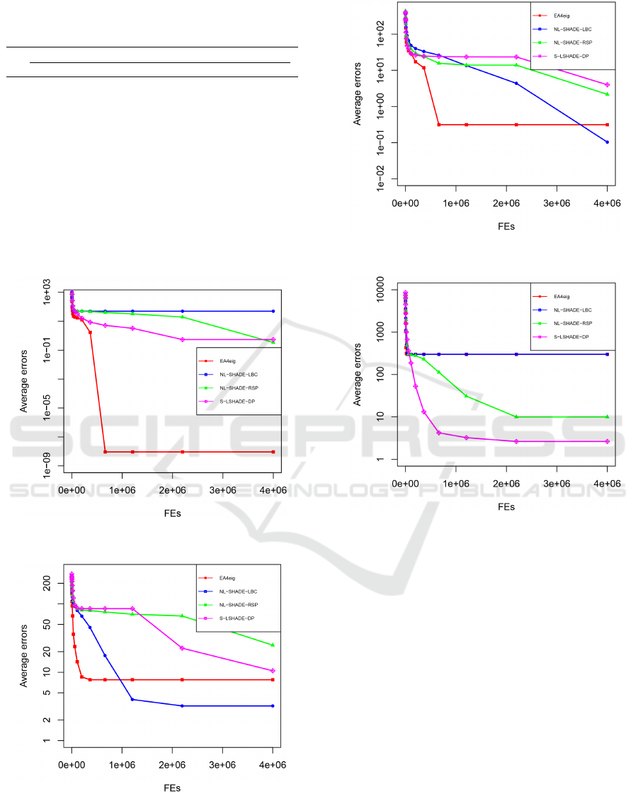
Table 9: Average errors obtained on the 12 benchmark func-

tions for the D = 10 for different stopping conditions for

S-LSHADE-DP.

S-LSHADE-DP

1E + 05 2E + 05 4E + 05 8E + 05

0 0 0 0

6.28 4.72 3.54 3.00

0 0 0 0

2.66E-01 2.60E-01 2.43E-01 2.28E-01

0 0 0 0

1.49E+00 1.89E-01 1.20E01 0.02E-01

2.29E+02 2.27E+02 2.22E+02 2.06E+02

1.37E+00 1.25E-02 0 0

0 0 0 0

1.62E+02 1.62E+02 1.61E+02 1.61E+02

Figure 1: The convergence graph of all four chosen solvers

on CEC 2022 Benchmark function f

for the D = 20.

Figure 2: The convergence graph of all four chosen solvers

on CEC 2022 Benchmark function f

for D = 20.

Figure 3: The convergence graph of all four chosen solvers

on CEC 2022 Benchmark function f

for D = 20.

Figure 4: The convergence graph of all four chosen solvers

on CEC 2022 Benchmark function f

for D = 20.

ACKNOWLEDGEMENTS

This work was supported by the Slovenian Research

Agency (Computer Systems, Methodologies, and In-

telligent Services) under Grant P2-0041.

REFERENCES

A. W. Mohamed, A. A. Hadi, A. K. Mohamed, P. Agrawal,

A. Kumar, P. N. Suganthan (December 2021). Prob-

lem Deﬁnitions and Evaluation Criteria for the CEC

2022 Special Session and Competition on Single Ob-

jective Bound Constrained Numerical Optimization.

Technical report, Nanyang Technological University,

Singapore.

A. W. Mohamed, A. A. Hadi, A. K. Mohamed, P. Agrawal,

A. Kumar, P. N. Suganthan (November 2020). Prob-

lem Deﬁnitions and Evaluation Criteria for the CEC

A Comparison of the State-of-the-Art Evolutionary Algorithms with Different Stopping Conditions

227

2021 Special Session and Competition on Single Ob-

jective Bound Constrained Numerical Optimization.

Technical report, Nanyang Technological University,

Singapore.

Bartz-Beielstein, T., Doerr, C., Berg, D. v. d., Bossek,

J., Chandrasekaran, S., Eftimov, T., Fischbach, A.,

Kerschke, P., La Cava, W., Lopez-Ibanez, M., et al.

(2020). Benchmarking in optimization: Best practice

and open issues. arXiv preprint arXiv:2007.03488.

Benavoli, A., Corani, G., Dem

sar, J., and Zaffalon, M.

(2017). Time for a change: a tutorial for compar-

ing multiple classiﬁers through Bayesian analysis. The

Journal of Machine Learning Research, 18(1):2653–

2688.

Biedrzycki, R., Arabas, J., and Warchulski, E. (2022). A

version of nl-shade-rsp algorithm with midpoint for

cec 2022 single objective bound constrained prob-

lems. In 2022 IEEE Congress on Evolutionary Com-

putation (CEC), pages 1–8. IEEE.

Birattari, M. and Dorigo, M. (2007). How to assess and

report the performance of a stochastic algorithm on a

benchmark problem: mean or best result on a number

of runs? Optimization letters, 1:309–311.

Biswas, S., Saha, D., De, S., Cobb, A. D., Das, S., and

Jalaian, B. A. (2021). Improving Differential Evolu-

tion through Bayesian Hyperparameter Optimization.

In 2021 IEEE Congress on Evolutionary Computation

(CEC), pages 832–840. IEEE.

Brest, J., Mau

cec, M. S., and Bo

skovi

c, B. (2016). iL-

SHADE: Improved L-SHADE algorithm for single

objective real-parameter optimization. In 2016 IEEE

Congress on Evolutionary Computation (CEC), pages

1188–1195. IEEE.

Brest, J., Zamuda, A., Fister, I., and Boskovic, B. (2014).

Some improvements of the self-adaptive jde algo-

rithm. In 2014 IEEE Symposium on Differential Evo-

lution (SDE), pages 1–8. IEEE.

Bujok, P. and Kolenovsky, P. (2022). Eigen crossover in

cooperative model of evolutionary algorithms applied

to cec 2022 single objective numerical optimisation.

In 2022 IEEE Congress on Evolutionary Computation

(CEC), pages 1–8. IEEE.

Calvo, B., Shir, O. M., Ceberio, J., Doerr, C., Wang, H.,

ack, T., and Lozano, J. A. (2019). Bayesian per-

formance analysis for black-box optimization bench-

marking. In Proceedings of the Genetic and Evolu-

tionary Computation Conference Companion, pages

1789–1797.

Carrasco, J., Garcia, S., Rueda, M., Das, S., and Herrera,

F. (2020). Recent trends in the use of statistical tests

for comparing swarm and evolutionary computing al-

gorithms: Practical guidelines and a critical review.

Swarm and Evolutionary Computation, 54:100665.

Cenikj, G., Lang, R. D., Engelbrecht, A. P., Doerr, C.,

Koro

sec, P., and Eftimov, T. (2022). Selector: se-

lecting a representative benchmark suite for repro-

ducible statistical comparison. In Proceedings of the

Genetic and Evolutionary Computation Conference,

pages 620–629.

Hansen, N., Auger, A., Ros, R., Mersmann, O., Tu

sar, T.,

and Brockhoff, D. (2021). COCO: A platform for

comparing continuous optimizers in a black-box set-

ting. Optimization Methods and Software, 36(1):114–

144.

Hansen, Nikolaus and Auger, Anne and Brockhoff, Dimo

and Tu

sar, Tea (2022). Anytime performance as-

sessment in blackbox optimization benchmarking.

IEEE Transactions on Evolutionary Computation,

26(6):1293–1305.

Herzog, J., Brest, J., and Bo

skovi

c, B. (2023). Analysis

based on statistical distributions: A practical approach

for stochastic solvers using discrete and continuous

problems. Information Sciences, 633:469–490.

Herzog, J., Brest, J., and Bo

skovi

c, B. (2022). Performance

Analysis of Selected Evolutionary Algorithms on Dif-

ferent Benchmark Functions. In Bioinspired Opti-

mization Methods and Their Applications: 10th Inter-

national Conference, BIOMA 2022, Maribor, Slove-

nia, November 17–18, 2022, Proceedings, pages 170–

184. Springer.

Jansen, T. (2020). Analysing stochastic search heuristics

operating on a ﬁxed budget. Theory of evolutionary

computation: recent developments in discrete opti-

mization, pages 249–270.

Kerschke, P., Hoos, H. H., Neumann, F., and Trautmann, H.

(2019). Automated algorithm selection: Survey and

perspectives. Evolutionary computation, 27(1):3–45.

Meng, Z., Zhong, Y., and Yang, C. (2021). Cs-de: Coop-

erative strategy based differential evolution with pop-

ulation diversity enhancement. Information Sciences,

577:663–696.

Nikolikj, A., Trajanov, R., Cenikj, G., Koro

sec, P., and

Eftimov, T. (2022). Identifying minimal set of Ex-

ploratory Landscape Analysis features for reliable

algorithm performance prediction. In 2022 IEEE

Congress on Evolutionary Computation (CEC), pages

1–8. IEEE.

Piotrowski, A. P., Napiorkowski, J. J., and Piotrowska,

A. E. (2020). Population size in particle swarm op-

timization. Swarm and Evolutionary Computation,

58:100718.

Ravber, M., Moravec, M., and Mernik, M. (2022). Primer-

java evolucijskih algoritmov implementiranih v ra-

zli

cnih programskih jezikih. Elektrotehniski Vestnik,

89(1/2):46–52. (In Slovene).

Stanovov, V., Akhmedova, S., and Semenkin, E. (2022).

NL-SHADE-LBC algorithm with linear parameter

adaptation bias change for CEC 2022 Numerical Op-

timization. In 2022 IEEE Congress on Evolutionary

Computation (CEC), pages 01–08. IEEE.

Tanabe, R. and Fukunaga, A. S. (2014). Improving the

search performance of SHADE using linear popula-

tion size reduction. In 2014 IEEE congress on evolu-

tionary computation (CEC), pages 1658–1665. IEEE.

sar, T., Hansen, N., and Brockhoff, D. (2017). Anytime

benchmarking of budget-dependent algorithms with

the COCO platform. In IS 2017-International mul-

ticonference Information Society, pages 1–4.

Van Cuong, L., Bao, N. N., Phuong, N. K., and Binh, H.

T. T. (2022). Dynamic perturbation for population di-

versity management in differential evolution. In Pro-

ECTA 2023 - 15th International Conference on Evolutionary Computation Theory and Applications

228

ceedings of the Genetic and Evolutionary Computa-

tion Conference Companion, pages 391–394.

Wolpert, D. H. and Macready, W. G. (1997). No free lunch

theorems for optimization. IEEE transactions on evo-

lutionary computation, 1(1):67–82.

Zhu, X., Ye, C., He, L., Zhu, H., and Chi, T. (2023). En-

semble of Population-Based Metaheuristics With Ex-

change of Individuals Chosen Based on Fitness and

Lifetime for Real Parameter Single Objective Opti-

mization.

A Comparison of the State-of-the-Art Evolutionary Algorithms with Different Stopping Conditions

229