TEAM: A Parameter-Free Algorithm to Teach Collaborative Robots

Motions from User Demonstrations

Lorenzo Panchetti

1 a

, Jianhao Zheng

1 b

, Mohamed Bouri

1 c

and Malcolm Mielle

2 d

Ecole Polytechnique F

erale de Lausanne (EPFL), Lausanne, Switzerland

Schindler AG, EPFL Lab, Lausanne, Switzerland

ﬂ

Keywords:

Learning from Demonstration, Cobots, Probabilistic Movement Primitives, Industrial Applications.

Abstract:

Learning from demonstrations (LfD) enables humans to easily teach collaborative robots (cobots) new motions

that can be generalized to new task conﬁgurations without retraining. However, state-of-the-art LfD methods

require manually tuning intrinsic parameters and have rarely been used in industrial contexts without experts.

We propose a parameter-free LfD method based on probabilistic movement primitives, where parameters are

determined using Jensen-Shannon divergence and Bayesian optimization, and users do not have to perform

manual parameter tuning. The cobot’s precision in reproducing learned motions, and its ease of teaching and

use by non-expert users are evaluated in two ﬁeld tests. In the ﬁrst ﬁeld test, the cobot works on elevator door

maintenance. In the second test, three factory workers teach the cobot tasks useful for their daily workﬂow.

Errors between the cobot and target joint angles are insigniﬁcant—at worst

0.28

deg—and the motion is

accurately reproduced—GMCC score of 1. Questionnaires completed by the workers highlighted the method’s

ease of use and the accuracy of the reproduced motion. Public implementation of our method and datasets are

made available online.

1 INTRODUCTION

Collaborative robots (cobots) are built to improve so-

ciety by helping people without replacing them. To

become an integrated part of our work, human work-

ers must be able to teach cobots new tasks in a short

time, making the robot a new tool in their toolbox.

However, programming the cobot is most of the time

done by experts and cobots cannot adapt to new task

conﬁgurations, instead repeating learned patterns.

Learning from demonstration (LfD) (Rana et al.,

2020)—a branch of learning focused on skill transfer

and generalization through a set of demonstrations—

enables cobots to learn and adapt motions from a set

of demonstrations. State-of-the-art LfD methods re-

quire either manually tuning intrinsic parameters or a

large amount of data, and have thus rarely been used

in industrial contexts without experts, since manual

tuning and data collection are time-consuming and

error-prone. In this paper, we present TEAM (

ach

a robot

rm to

ove), a novel method to learn from

https://orcid.org/0009-0004-9657-7249

https://orcid.org/0000-0003-4430-3049

https://orcid.org/0000-0003-1083-3180

https://orcid.org/0000-0002-3079-0512

demonstrations without manual tuning of intrinsic pa-

rameters during training.

The main contributions of this paper are:

•

A parameter-free framework to learn motions from

a set of demonstrations, using a generative model

to ﬁnd a generalized trajectory, and attractor land-

scapes to reproduce the motion between different

start and target joint angles.

•

An optimization strategy of the attractor land-

scape’s intrinsic parameters through Bayesian op-

timization.

•

Improvement on the selection of the number of

Gaussian Mixture Models through a series of one-

tailed Welch’s t-tests, based on the Jensen-Shannon

divergence.

•

Experimental validation of TEAM in two ﬁeld tests

showing that our method can be used by non-expert

robot users.

A complete overview of the methodology is shown

in Figure 1.

570

Panchetti, L., Zheng, J., Bouri, M. and Mielle, M.

TEAM: A Parameter-Free Algorithm to Teach Collaborative Robots Motions from User Demonstrations.

DOI: 10.5220/0012159700003543

In Proceedings of the 20th International Conference on Informatics in Control, Automation and Robotics (ICINCO 2023) - Volume 1, pages 570-577

ISBN: 978-989-758-670-5; ISSN: 2184-2809

Dynamic Time

Warping

Demonstrations:

Gaussian mixture

model (GMM) and

regression (GMR)

Number of components

K found using JS

divergence approach

Damped Spring Models

Model parameters α

and N found through

Bayesian optimization

Attractor landscape TrajectoryStart and target joint angles

Aligned demonstrations

GMR

Model parameters

Figure 1: A set of demonstrations is recorded by a user

and the motion is generalized through GMR. The system is

modelled as a set of damped spring models that generalize

the motion. Given start and target joint angles, model’s

parameters are used to generate new trajectories reproducing

the motion taught by demonstrations. All system parameters

are automatically optimized, and no expert knowledge is

needed.

2 RELATED WORK

Rana et al. (2020) present a large-scale study bench-

marking the performance of motion-based LfD ap-

proaches and show that Probabilistic Movement Primi-

tives (ProMP) (Paraschos et al., 2013) methods are the

most consistent on tasks with positional constraints.

ProMP is a general probabilistic framework for learn-

ing movement primitives that allows new operations,

including conditioning and adaptation to changed task

variables.

Calinon et al. (2007) ﬁt a mixture of Gaussians

on a set of demonstrations and generalize the motion

through Gaussian Mixture Regression (GMR) (Cohn

et al., 1996). Trajectories are computed by optimiz-

ing an imitation performance metric. However, joint

conﬁgurations are not constrained to the demonstra-

tion space, which can lead to the exploration of unsafe

areas.

Kulak et al. (2021) propose to use Bayesian

Gaussian mixture models to learn ProMP. While their

method reduces the number of demonstrations needed

to learn a representation with generalization capabili-

ties, the method parameters must be manually set for

all experiments.

Ijspeert et al. (2013) and Schaal (2006) use Dynam-

ical Movement Primitives (DMP) to model complex

motions through nonlinear dynamical systems. DMP

is scale and temporal invariant, convergence is proven,

but the parameters of the system must be manually

tuned.

Pervez et al. (2018) propose a method that general-

izes motion outside the demonstrated task space. Each

demonstration is associated with a dynamical system,

and learning is formulated as a density estimation prob-

lem. However, parameters must be set empirically for

all dynamical systems.

Recent works have leveraged advances in deep

learning. To tackle the challenging problem of model

collapse, (Zhou et al., 2020) propose using a mixture

density network (MDN) that takes task parameters as

input and provides a Gaussian mixture model (GMM)

of the MP parameters. During training, their work

introduces an entropy cost to achieve a more balanced

association of demonstrations to GMM components.

Pahi

cet al. (2020) propose to train a neural net-

work to output the parameters of the DMP model from

an image, before learning the associated forcing term.

Pervez et al. (2017) use deep neural networks to learn

the forcing terms of the DMP model for vision-based

robot control. Both methods involve a convolutional

neural network learning task-speciﬁc features from

camera images. Sanni et al. (2022) estimate the corre-

lation between visual information and ProMP weights

for reach-to-palpate motion. The average error in task

space is around 3 to 5 centimeters which is too high for

our application. Yang et al. (2022) use reinforcement

learning to learn a latent action space representing

the skill embedding from demonstrated trajectories

for each prior task. Tosatto et al. (2020) provide a

complete framework for sample-efﬁcient off-policy

RL optimization of MP for robot learning of high-

dimensional manipulation skills. All methods based on

deep or reinforcement learning require a large amount

of data. E.g., Sanni et al. (2022) show the robot the

reach-to-palpate motion 500 times, Pervez et al. (2017)

acquire 50 demonstrations for a single task, and Yang

et al. (2022) uses around 80K trajectories.

3 METHOD

3.1 Overview

To learn a motion, a set of demonstrations is ﬁrst col-

lected by the user. In our work, the cobot is taught by

manual guidance—see the image in the demonstration

box of Figure 1. A demonstration stores the cobot’s

joint angles recorded while the cobot is shown the

task and the robot is controlled in joint space to avoid

singularities during the motion of the redundant robot

arm. As in previous work by Calinon et al. (2007),

demonstrations are aligned in time using dynamic time

warping (Sakoe and Chiba, 1978).

The ﬁrst step of our method consists in ﬁnding the

best Gaussian mixture model (GMM) ﬁt on the demon-

TEAM: A Parameter-Free Algorithm to Teach Collaborative Robots Motions from User Demonstrations

571

strations dataset and calculates the Gaussian Mixture

Regression (GMR)—i.e. the generalized trajectory.

Section 3.2 shows how to use the Jensen-Shannon

(JS) divergence (Lin, 1991) to ﬁt the GMM and GMR

without user input. From the GMR, the motion is rep-

resented as a set of damped spring models; Section 3.4

shows how to estimate the optimal parameters of the

models through Bayes optimization. Finally, the op-

timal motion is computed by the attractor landscape,

given initial and goal cobot joint angles.

3.2 Gaussian Mixture Model and

Gaussian Mixture Regression

Given a set of demonstrations, a GMM is ﬁtted on

each degree of freedom—each of the cobot’s joints.

Maximum likelihood estimation of the mixture param-

eters is done using Expectation Maximization (EM)

(Dempster et al., 1977).

The number of mixture model components

critical to obtaining a GMM leading to a smooth GMR.

While Calinon et al. (2007) used the BIC criterion

to determine the optimal value

—denoted

∗

in our

work—Pervez et al. (2017) showed that BIC overﬁts

the dataset without a manually tuned regularization

factor. We propose a novel strategy to ﬁnd

∗

without

any manual thresholds, based on cross validation, the

JS divergence, and statistical analysis.

For

k = 2

until

k = c

—with

the maximum num-

ber of components in the GMM—50 cross validations

are performed over the demonstration dataset using the

JS divergence as a measure of similarity between the

GMMs generated from the train and test splits. The

mean

and standard deviation

of the JS diver-

gences for each

are stored in the set

s(k) → (m

, s

)

∗

is initialized as the value in

with the minimum

. For each key

k ∈ s

, a serie of one-tailed Welch’s

t-tests (Welch, 1947) with

α = 0.05

—i.e. there is a 5%

chance that the results occurred at random—is used

to evaluate whether

is a more optimal number of

components than the current value of

∗

. First, we test

if the JS divergence of

is strictly greater than that of

∗

. The null hypothesis H1 and alternative hypothesis

H2 are:

Hypothesis 1 (H1): k − k

∗

≤ 0

Hypothesis 2 (H2): k

∗

− k < 0

If the null hypothesis is rejected,

is strictly greater

than

∗

and

is not the optimal number of components.

If we fail to reject the null hypothesis, we then test if

is strictly less than

∗

. The null hypothesis H3 and

alternative hypothesis H4 are:

Data: demonstrations set D

Result: k

∗

1 s ← empty map;

2 for k = 2 until k = c do

3 res ← empty list;

4 for 1 to 50 do

5 Sample datapoints of D in two equal

sets D

and D

;

6 G

← GMM with k components ﬁtted

on D

;

7 G

← GMM with k components ﬁtted

on D

;

8 Add JSdivergence(G

, G

) to res;

9 end

10 m

, s

← mean(res), std(res);

11 s(k) ← (m

, s

);

12 end

13 k

∗

← component in s with the lowest mean;

14 for key k, value (m

, s

) ∈ s do

15 if H1 is not rejected then

16 if H3 is rejected or s

< s

∗

then

17 k

∗

← k;

18 end

19 end

20 end

21 return k

∗

Algorithm 1: Algorithm used to determine the best number

of components for the GMM.

Hypothesis 3 (H3): k

∗

− k ≤ 0

Hypothesis 4 (H4): k − k

∗

< 0

If the null hypothesis is rejected,

∗

is strictly greater

than

, and

is the optimal number of components. If

we failed to reject both H1 and H3, no conclusions as

to whether

∗

is the best estimate can be drawn,

and

∗

is set to the most stable number of components:

∗

= k if and only if s

is lower than s

∗

The process to determine the optimal number of

Gaussians is detailed in Algorithm 1.

3.3 Damped Spring Model

TEAM uses the damped spring model formulated by

Ijspeert et al. (2013): :

τ˙z = α

(β

(g − y) −z) + f

˙y = z

(1)

where

is a time constant,

is the nonlinear forcing

term,

and

are positive constants, and

is the

target joint angles. The forcing term

of Equation (1)

is used to produce a speciﬁc trajectory—i.e. the GMR.

Since

is a nonlinear function, it can be represented

ICINCO 2023 - 20th International Conference on Informatics in Control, Automation and Robotics

572

as a normalized linear combination of basis functions

(Bishop, 2006):

f (x) =

∑

i=1

(x)ω

∑

i=1

(x)

(g − y

)v (2)

where

are ﬁxed radial basis functions,

are the

weights learned during the ﬁt,

is the goal joint an-

gles, and

is the system velocity.

is the number

of ﬁxed radial basis function kernels

(x)

. Detailed

derivations, and methods to compute

and the joint

dynamics, are found in Ijspeert et al. (2013).

3.4 Parameters Optimization

For

to monotonically converge towards the target

, the system must be critically damped on the GMR

by choosing the appropriate values of

and

. As

shown by Ijspeert et al. (2013),

can be expressed

with respect to

4β

= α

. Thus, only two pa-

rameters control the tracking of the reference and the

stability: the number of radial basis functions

and

the constant

. In the previous state-of-the-art (e.g.

Ijspeert et al. (2013) and Pervez et al. (2018)),

and

are empirically chosen by the user. Instead, TEAM

uses Bayesian optimization (BO) (Garnett, 2022) to

determine α

and N and avoid manual tuning.

The error to minimize is the sum of both the root

mean squared error with respect to the GMR and the

distance of the trajectory endpoint with respect to the

goal reference:

f (α

, N) =

∑

t=1

(y(α

, N, t) − y

(t))

+ ||y(α

, N, T ) − y

(T )||

(3)

where

y(α

, N, t)

is the joint angles at time

obtained

with DMP parameters

and

(t)

is the GMR

joint angles at time

, and

|| · ||

is the

-norm. The

acquisition function is the expected improvement (EI):

(x) := E

[ f (x) − f

∗

] (4)

where

[·|x

1:i

]

indicates the expectation taken under

the posterior distribution given evaluations of

f (x)

x = x

, ...,x

. The acquisition function retrieves the

point in the search space that corresponds to the largest

expected improvement and uses it for the next eval-

uation of the objective function

f (x)

. The point

minimizing the value of

f (x)

corresponds to the op-

timal combination of

and

. The optimization is

stopped when two successive query points are equal.

rail

opening tool

lock

Figure 2: The cobot faces the test elevator door used for

evaluation of TEAM in a maintenance scenario.

4 EVALUATION

We evaluate our method in two real-world scenarios,

using a 6-axis ABB GoFa CRB 15000 cobot

—pose

repeatability at the maximum reach and load is 0.05

mm. In the ﬁrst scenario, the cobot works alone to

do maintenance operations on an elevator door. This

scenario is used to evaluate the stability of the method—

both the parameter selection and its robustness to start

and goal angle changes. The second scenario pertains

to the ease of use of our method for non-expert users:

three Schindler workers teach the cobot a set of tasks

needed to drill elevator pieces on Schindler’s factory

line.

The desired workﬂow for ﬁeld technicians is one

where, for a given task, the cobot ﬁrst learns the motion

and then reproduces the motion on the factory line

without having to be trained again. Hence, for each

task, a set of demonstrations is recorded by a user and

the cobot learns the motion using TEAM. Then, using

the previously trained model, the cobot reproduces the

task multiple times with different start joint angles.

To measure the cobot’s accuracy in reaching the

target joint angles, we measure the mean absolute er-

ror

between the goal joint

and actual end joint

angles:

∑

i=1

− g

(5)

with

the number of joints. To measure the quality

of the reproduced motion, we use the Generalized

Multiple Correlation Coefﬁcient (GMCC) proposed by

Urain et al. (2019), a measure of similarities between

trajectories that is invariant to linear transformations.

Code, datasets, and metrics can be found online.

4.1 Door Maintenance Dataset

The 5 tasks of elevator door maintenance dataset:

https://new.abb.com/products/robotics/

collaborative-robots/crb-15000

https://github.com/SchindlerReGIS/team

TEAM: A Parameter-Free Algorithm to Teach Collaborative Robots Motions from User Demonstrations

573

Table 1: JS divergence repeatability over 50 runs.

Task T1 T2 T3 T4 T5

Median nb GMM

5 ±0.40 3 ±0 4 ±0 3 ± 0 4 ±0.27

Table 2: Comparison between grid search (GS) and Bayesian

optimization (BO). Statistics over 50 runs.

Task T1 T2 T3 T4 T5

GS minimum

12.84 73.91 30.88 36.58 26.44

BO minimum

12.84

±0

74.22

±0.61

30.98

±0.40

36.68

±0.27

26.44

±0.05

GS time [s]

2348.97 2600.96 2427.34 2149.50 1848.20

BO median

time [s]

19.39

±3.63

27.40

±10.17

12.40

±2.40

26.11

±18.54

12.53

±1.99

GS calls

3750 3750 3750 3750 3750

BO calls

23.14

±3.88

34.20

±10.85

16.96

±2.73

32.98

±18.97

20.14

±2.58

• T 1

: open and lock the door using a custom opening

tool. The lock is now in the middle of the rail.

• T 2: grab the cleaning tool.

• T 3

: clean the rail while avoiding the lock. The

cobot must aim for both ends of the rail with the

brush since most dust accumulates there.

• T 4: drop the cleaning tool on its support.

• T 5

: grab the opening tool, close the door, and

combine the two pieces of the opening tool.

The maintenance setup can be seen in Figure 2.

4.1.1 Evaluation of the Parameters’

Repeatability

A repeatability analysis of the parameters

, and

is done on the data collected for the door maintenance

scenario.

Repeatability of

Using the JS Divergence: the

method described in Section 3.2 is run 50 times for

each task in the maintenance dataset—with a minimum

of 2 Gaussians and a maximum of 9. As seen in Ta-

ble 1, the median number of Gaussians for each dataset

varies only by a small standard deviation, showing that

the selection of the number of Gaussian components

is stable.

Damped Spring Model Parameters: we compare BO

with grid search (GS) for 50 runs per task in the main-

tenance dataset. One can see in Table 2 that BO con-

verges 100 times faster than GS and to the same global

optimum. Optimization took an average of 19.57s on

an Intel Core i5 10

Gen and there is a reduction by

a factor of at least 100 in the number of iterations

needed—it should be noted that larger standard devi-

ations in the running time are usually due to larger

outliers with a median time around 20s.

In conclusion, we ﬁnd that the JS divergence and

BO lead to a stable selection of

, and

, and can

be used as sensible replacements for the manual tuning

previously done by expert users.

4.1.2 Adaptability

Table 3 shows the number of demonstrations recorded

for each task, with the average training times and error

metrics.

The complexity of DTW is

O((M − 1)L

)

, with

the number of demonstrations in the dataset and

the longest demonstration length, GMM and GMR are

O(KBD

)

where

is the number of datapoints in the

dataset,

the data dimensionality, and

the number

of GMM components. The Gaussian Process of the

BO is

O(R

)

with

being the number of function

evaluations—Table 2 shows that

is at worse around

34.20 ± 10.85

. As seen in Table 3, in the maintenance

scenario, the maximum training time is under 4min—

the longest training time is 203.33 ± 4.32s for T 2.

Once a model is trained, the accuracy of the re-

produced trajectory is evaluated by computing 30 re-

productions and calculating the GMCC between the

reproduced trajectory and the GMR. For each repro-

duction, the target joint angles are the same as the last

joint angles of the GMR, and the start joint angles are

the same as the GMR, with the addition of a zero mean

Gaussian noise with standard deviation of

, and

degrees. For each noise value, the average GMCC

and

per task are shown in Table 3. One can see that,

regardless of the noise value, GMCCs and

are very

close to

and

respectively, showing that the cobot

accurately reproduces the demonstrated motion and

reaches the target joint angles. E.g., Figure 3 shows

the regression trajectory and reproduction per joint

with Gaussian noise with standard deviation of 20 deg:

the trajectory of each joint is conserved regardless of

the noise added to the start joint angles.

4.2 Field Tests and User Study

To validate that the cobot can be used by non-expert

users in a professional setting, we conducted ﬁeld tests

at the Schindler headquarters with three Schindler ﬁeld

workers working on the production line. None of the

workers had worked with a cobot before. To ensure

realism of the tasks, the ﬁeld workers designed four

test scenarios that would reduce their workload if the

robot can easily be taught how to perform the task:

• F1

: ﬁnd a metal piece, grab and place it on a

drilling machine.

• F2

: ﬁnd a metal piece, grab and place it on a

drilling machine while avoiding an obstacle.

ICINCO 2023 - 20th International Conference on Informatics in Control, Automation and Robotics

574

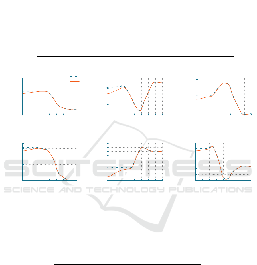
Table 3: This table presents the training time and error metrics for the maintenance tasks— 30 runs per task.

Noise Task T1 T2 T3 T4 T5

Number of demonstrations 6 4 4 4 3

Average demonstration duration [s] 33.19 ± 2.38 36.37± 2.28 32.93 ± 3.00 28.17± 3.33 26.19 ± 1.05

Training time [s] 184.08 ± 2.45 203.33 ± 4.32 185.82 ± 3.07 162.89 ± 4.56 148.59 ± 4.51

GMCC 1.00 ± 0.00 1.00 ± 0.00 1.00 ± 0.00 1.00 ± 0.00 1.00 ± 0.00

1 deg e

[deg] 0.14 ± 0.00 0.19 ± 0.00 0.30 ± 0.00 0.01 ± 0.00 0.05 ± 0.00

GMCC 1.00 ± 0.00 1.00 ± 0.00 1.00 ± 0.00 1.00 ± 0.00 1.00 ± 0.00

5 deg e

[deg] 0.14 ± 0.00 0.19 ± 0.00 0.30 ± 0.00 0.01 ± 0.00 0.05 ± 0.00

GMCC 1.00 ± 0.00 1.00 ± 0.00 1.00 ± 0.00 1.00 ± 0.00 1.00 ± 0.00

10 deg e

[deg] 0.14 ± 0.00 0.19 ± 0.00 0.28 ± 0.00 0.01 ± 0.00 0.05 ± 0.00

GMCC 1.00 ± 0.00 1.00 ± 0.00 1.00 ± 0.00 1.00 ± 0.00 1.00 ± 0.00

20 deg e

[deg] 0.14 ± 0.00 0.19 ± 0.00 0.28 ± 0.00 0.015 ± 0.00 0.05 ± 0.00

−80

−50

−20

0 5 10 15 20 25 30 35 40

joint angle (deg)

time (s)

regression

reproduction

(a) Joint 1

−20

−10

0 5 10 15 20 25 30 35 40

time (s)

(b) Joint 2

−30

−10

0 5 10 15 20 25 30 35 40

time (s)

−80

−60

−40

−20

0 5 10 15 20 25 30 35 40

joint angle (deg)

time (s)

(d) Joint 4

−85

−80

−75

−70

−65

−60

−55

−50

−45

−40

0 5 10 15 20 25 30 35 40

time (s)

(e) Joint 5

120

150

180

0 5 10 15 20 25 30 35 40

time (s)

(f) Joint 6

Figure 3: Reproduction and regression joint angles evolution on an example of the

T 1

task. Start joint angles of the reproduction

are computed by adding Gaussian noise with 20deg standard deviation on the regression initial joint angles. The reproduced

trajectory reproduces the regression’s motion and reach the target joint angles.

Table 4: This table presents error metrics for the factory scenario—dataset consisted of 3 to 4 demonstrations.

Task F1 F2 F3 F4

Number of reproductions 31 30 33 20

GMCC 0.99 ± 0.02 0.99 ± 0.00 0.99 ± 0.01 1.00 ± 0.00

Joints error e

[deg] 0.00 ± 0.00 0.02 ± 0.02 0.04 ± 0.05 0.02 ± 0.02

• F3

: ﬁnd a metal frame, grab and place it on a

drilling machine while rotating the piece.

• F4

: ﬁnd a wooden plank, grab one side while the

worker grabs the other, and place it together on a

drilling machine.

A custom app on a smartphone was used by the work-

ers to interact with the robot in an intuitive manner.

The app consists of two main pages: one to record

demonstrations and train a model, and another page

to give the robot a target position and start the task

reproduction. After a short training on how to use the

app, three to ﬁve demonstrations were recorded per

user, per task. To calculate the metric, each task was

reproduced around 10 times per user, apart from

where only two users participated—hence

repro-

ductions. Detection of the different objects is done

using template matching (Brunelli, 2009).

Table 4 shows the GMCC and

for all tasks, cal-

culated for 30 reproductions of the motion for each

task. The error metrics results are similar to the ones

presented in Section 4.1, with GMCC averaging

0.99

and

deg; demonstrating accurate task reproduc-

tion in a realistic scenario.

TEAM: A Parameter-Free Algorithm to Teach Collaborative Robots Motions from User Demonstrations

575

(a) User 1, day 1

(b) User 1, day 2

(d) User 3

Figure 4: After use, the cobot is evaluated by each of the users on: safety (S), easiness to teach (T), entertainment (E), reaching

the target joint angles (A), and task completion (C). In blue the results for the task F1, F2, and F3, and in red the results for the

collaborative task F4. One can see the collaborative task, where the user carries a piece of wood with the robot, is more difﬁcult

than other task were the cobot works next to the user.

The ﬁeld tests were conducted over two days and,

at the end of each day, the workers answered a ques-

tionnaire to evaluate the cobot’s performance. In the

survey, users rate the following statements on a scale

from 1 to 5, corresponding to strongly disagree, dis-

agree, neutral, agree, and strongly agree:

• The cobot learned the correct motion.

• I felt safe operating the cobot.

• The cobot reached the goal point accurately.

• Teaching the cobot a motion was simple.

• Teaching the cobot a motion was entertaining.

The radar plots in Figure 4 present survey results.

While users showed satisfaction with the cobot’s preci-

sion and motion performance, the complexity of hold-

ing the beam and moving the cobot while showing

the motion in F4 led to a lower score for easiness of

teaching compared to other tasks.

5 LIMITATIONS AND FUTURE

WORK

TEAM doesn’t consider elements of the environment

during the motion. This create confusion for the work-

ers not understanding why the cobot does not avoid

obstacles, making it harder for them to trust the cobot.

Future work will look at integrating visual information

through cameras to update the motion depending on

the environment.

Another way that TEAM could be improved is by

being able to update the attractor landscape of a motion

incrementally. Future work will look into making

the process incremental, giving workers the ability to

correct existing motions learned by the cobot.

6 SUMMARY

A method to learn motions from demonstrations requir-

ing no manual parameter tuning has been developed.

Given a set of demonstrations aligned in time, the

motion is generalized using GMM and the reference

trajectory is extracted with GMR. Since BIC criterion

can lead to over-ﬁtting of the GMM, it is proposed to

instead use the Jensen-Shannon divergence to deter-

mine the optimal number of GMM components. The

cobot DOFs are represented as damped spring models

and the forcing term is learned to adapt the motion to

different start and goal joint poses. Parameters of the

spring model are found using Bayesian optimization.

TEAM is extensively evaluated in two ﬁeld tests

where the cobot performs tasks related to elevator door

maintenance, and works in realistic scenarios with

Schindler ﬁeld workers. The precision in joint angles

and motion reproduction quality are evaluated, and the

experiments show that the cobot accurately reproduces

the motions—GMCC and mean average error for the

ﬁnal joint angles are around

and

respectively. Fur-

thermore, feedback collected from the ﬁeld workers

shows that the cobot is positively accepted since it is

easy to teach and easy to use.

REFERENCES

Bishop, C. M. (2006). Pattern recognition and machine

learning (information science and statistics).

Brunelli, R. (2009). Template matching techniques in com-

puter vision: Theory and practice.

Calinon, S., Guenter, F., and Billard, A. (2007). On learning,

representing, and generalizing a task in a humanoid

robot. IEEE Transactions on Systems, Man, and Cy-

bernetics, Part B (Cybernetics), 37:286–298.

Cohn, D. A., Ghahramani, Z., and Jordan, M. I. (1996).

Active learning with statistical models. In NIPS.

ICINCO 2023 - 20th International Conference on Informatics in Control, Automation and Robotics

576

Dempster, A. P., Laird, N. M., and Rubin, D. B. (1977).

Maximum likelihood from incomplete data via the em

algorithm. Journal of the Royal Statistical Society:

Series B (Methodological), 39(1):1–22.

Garnett, R. (2022). Bayesian Optimization. Cambridge

University Press. in preparation.

Ijspeert, A. J., Nakanishi, J., Hoffmann, H., Pastor, P., and

Schaal, S. (2013). Dynamical Movement Primitives:

Learning Attractor Models for Motor Behaviors. Neu-

ral Computation, 25(2):328–373.

Kulak, T., Girgin, H., Odobez, J.-M., and Calinon, S. (2021).

Active learning of bayesian probabilistic movement

primitives. IEEE Robotics and Automation Letters,

6:2163–2170.

Lin, J. (1991). Divergence measures based on the shannon

entropy. IEEE Transactions on Information Theory,

37(1):145–151.

Pahi

c, R., Ridge, B., Gams, A., Morimoto, J., and Ude,

A. (2020). Training of deep neural networks for the

generation of dynamic movement primitives. Neural

networks : the ofﬁcial journal of the International

Neural Network Society, 127:121–131.

Paraschos, A., Daniel, C., Peters, J., and Neumann, G.

(2013). Probabilistic movement primitives. In NIPS.

Pervez, A. and Lee, D. (2018). Learning task-parameterized

dynamic movement primitives using mixture of gmms.

Intelligent Service Robotics, 11:61–78.

Pervez, A., Mao, Y., and Lee, D. (2017). Learning deep

movement primitives using convolutional neural net-

works. 2017 IEEE-RAS 17th International Conference

on Humanoid Robotics (Humanoids), pages 191–197.

Rana, M. A., Chen, D., Ahmadzadeh, S. R., Williams, J.,

Chu, V., and Chernova, S. (2020). Benchmark for

skill learning from demonstration: Impact of user ex-

perience, task complexity, and start conﬁguration on

performance. 2020 IEEE International Conference on

Robotics and Automation (ICRA), pages 7561–7567.

Sakoe, H. and Chiba, S. (1978). Dynamic programming

algorithm optimization for spoken word recognition.

IEEE Transactions on Acoustics, Speech, and Signal

Processing, 26:159–165.

Sanni, O., Bonvicini, G., Khan, M. A., L

opez-Custodio,

P. C., Nazari, K., and AmirM.Ghalamzan, E. (2022).

Deep movement primitives: toward breast cancer ex-

amination robot. ArXiv, abs/2202.09265.

Schaal, S. (2006). Dynamic Movement Primitives -A Frame-

work for Motor Control in Humans and Humanoid

Robotics, pages 261–280. Springer Tokyo, Tokyo.

Tosatto, S., Chalvatzaki, G., and Peters, J. (2020). Con-

textual latent-movements off-policy optimization for

robotic manipulation skills. 2021 IEEE International

Conference on Robotics and Automation (ICRA), pages

10815–10821.

Urain, J. and Peters, J. (2019). Generalized multiple correla-

tion coefﬁcient as a similarity measurement between

trajectories. In 2019 IEEE/RSJ International Confer-

ence on Intelligent Robots and Systems (IROS), pages

1363–1369.

Welch, B. L. (1947). The generalization of ‘student’s’ prob-

lem when several different population varlances are

involved. Biometrika, 34:28–35.

Yang, Q., A. Stork, J., and Stoyanov, T. (2022). Mpr-

rl: Multi-prior regularized reinforcement learning for

knowledge transfer. IEEE Robotics and Automation

Letters, pages 1–8.

Zhou, Y., Gao, J., and Asfour, T. (2020). Movement primitive

learning and generalization: Using mixture density

networks. IEEE Robotics & Automation Magazine,

27:22–32.

TEAM: A Parameter-Free Algorithm to Teach Collaborative Robots Motions from User Demonstrations

577