Lyapunov Function Computation for Linear Switched Systems:
Comparison of SDP and LP Approaches
Stefania Andersen
1 a
, Elias August
2 b
, Sigurdur Hafstein
1 c
and Jacopo Piccini
2 d
1
University of Iceland, Faculty of Physical Sciences, Dunhagi 5, 107 Reykjavik, Iceland
2
Reykjavik University, Department of Engineering, Menntavegur 1, 102 Reykjavik, Iceland
Keywords:
Switched Systems, Lyapunov Functions, Semidefinite Programming, Linear Programming, Visualisation
Software.
Abstract:
For a switched system, of which each subsystem is linear, the exponential stability of the origin is equivalent
to the existence of a common Lyapunov function (CLF) for all the subsystems. A popular approach to search
for the latter is by means of solving a linear matrix inequality (LMI) using semidefinite programming (SDP).
Another approach is to use linear programming (LP). The contribution of this work is twofold. First, we
compare the SDP approach to the LP approach, with and without a certain preconditioning of system matrices.
And, second, we present a software tool to visualise the conditions for a CLF. As the problem of investigating
the stability of the origin is a very difficult one and sufficient and necessary conditions using the system
matrices are only known for exponential stability of planar systems, a tool to visualise the original data in
some meaningful form is potentially of great use for the full understanding of the problem.
1 INTRODUCTION
In science and engineering, one often uses ordinary
differential equations (ODEs) for modelling, that is,
the temporal behaviour of the state variables is quan-
tified through a differential equation of the following
form,
˙
x = f(x), x ∈ R
n
. (1)
If system (1) has an equilibrium point x
0
, that is,
f(x
0
) = 0, which, without loss of generality, can be
assumed to be at the origin, then one often studies the
linearised system given by
˙
x = Ax, A := Df(0), x ∈R
n
. (2)
According to the Hartman-Grobman theorem (Gr
¨
une
and Junge, 2016), its solutions have the same qual-
itative behaviour close to the origin as system (1)
whenever the real parts of the eigenvalues of Df(0)
are nonzero; here Df(0) ∈R
n×n
denotes the Jacobian-
matrix of f at the origin.
In different engineering applications, such as
power electronics, automotive control, robotics, and
a
https://orcid.org/0000-0001-6747-775X
b
https://orcid.org/0000-0001-9018-5624
c
https://orcid.org/0000-0003-0073-2765
d
https://orcid.org/0000-0002-4180-8140
air traffic control (Veer and Poulakakis, 2020), it is
useful to consider a switched linear system of the fol-
lowing form,
˙
x = A
m
x, m ∈ P , x ∈ R
n
. (3)
The switching between the systems
˙
x = A
m
x is
modelled through switching signal σ: [0, ∞) → P .
Moreover, in hybrid systems, switching is due to
the interaction between the dynamics of individual
continuous-time subsystems and the discrete-time dy-
namics of the switching (Goebel et al., 2012). An-
other common source of switched systems is uncer-
tainty quantification in continuous-time systems and
the associated differential inclusions (Aubin and Cel-
lina, 1984; Clarke, 1990). In this paper, we will only
consider arbitrary switching between a finite number
of systems; that is, P is finite and σ: [0, ∞) →P is ar-
bitrary, except for the (technical) assumption that the
number of switching times is finite on any finite time-
interval.
The transition matrix for system (2) is t 7→exp[At];
that is, a solution starting at ξ ∈R
n
at time zero will be
at exp[At]ξ at time t. Correspondingly, the transition
matrix for (3) with switching signal σ is
t 7→exp[A
σ(t
k
)
(t −t
k
)] ·exp[A
σ(t
k−1
)
(t
k
−t
k−1
)]·
···exp[A
σ(t
1
)
(t
2
−t
1
)] ·exp[A
σ(t
0
)
(t
1
−t
0
)],
Andersen, S., August, E., Hafstein, S. and Piccini, J.
Lyapunov Function Computation for Linear Switched Systems: Comparison of SDP and LP Approaches.
DOI: 10.5220/0012084100003546
In Proceedings of the 13th International Conference on Simulation and Modeling Methodologies, Technologies and Applications (SIMULTECH 2023), pages 61-70
ISBN: 978-989-758-668-2; ISSN: 2184-2841
Copyright
c
 2023 by SCITEPRESS – Science and Technology Publications, Lda. Under CC license (CC BY-NC-ND 4.0)
61

where the t
0
,t
1
,t
2
, . . . ,t
k
are the switching times and
t > t
k
> t
k−1
> . . . > t
1
> t
0
= 0.
Asymptotic stability of system (2) is equivalent to
exponential stability; that is, there exist constants α >
0 and c ≥ 1 such that
∥φ(t,ξ)∥≤ c∥ξ∥exp[−tα] for all t ≥ 0, (4)
where φ(t, ξ) := exp[At]ξ. Note that the origin is
asymptotically stable, if and only if the real-parts of
all eigenvalues of A are negative. In this case, matrix
A is said to be Hurwitz.
The origin is said to be exponentially stable for
switched system (3) under arbitrary switching if and
only if, for every switching signal σ with a finite num-
ber of switching times on every finite interval, there
exist constants α > 0 and c ≥ 1 such that inequality
(4) holds for
φ
σ
(t,ξ) :=exp[A
σ(t
k
)
(t −t
k
)] ·exp[A
σ(t
k−1
)
(t
k
−t
k−1
)]
···exp[A
σ(t
1
)
(t
2
−t
1
)] ·exp[A
σ(t
0
)
(t
1
−t
0
)]ξ.
For planar systems (n = 2) and switching only be-
tween two different systems (|P | = 2), the exponen-
tial stability of the origin can be characterised through
matrices A
1
and A
2
, where P = {1, 2}. The ori-
gin is exponentially stable if and only if all pair-
wise convex combinations of A
1
, A
2
, A
−1
1
, and A
−1
2
are Hurwitz (Cohen and Lewkowicz, 1993; Liber-
zon, 2003). However, unless the matrices A
m
have
some very special structure, for instance, if they all
commute (Agrachev and Liberzon, 2001), determin-
ing stability remains an open problem.
A sufficient condition for exponential stability of
the origin of (3) is the existence of a quadratic com-
mon Lyapunov function (QCLF) for the subsystems.
Computing a QCLF numerically by solving the linear
matrix inequality (LMI) (Khalil, 2002; Boyd et al.,
1994) given by
P ≻ 0, PA
m
+ A
T
m
P ≺ 0, ∀m ∈ P , (5)
is a frequent approach. Here, P ≻ 0 means that
P ∈ R
n×n
is symmetric and positive definite . How-
ever, even in the case n = |P | = 2 it is possible that an
arbitrarily switched system has an exponentially sta-
ble equilibrium at the origin, but there does not exist a
QCLF for the system. Numerous methods to compute
different kinds of common Lyapunov function (CLF)
have been proposed in the literature; for example,
see (Giesl and Hafstein, 2015). One method is to use
linear programming (LP) to parametrise piecewise
linear Lyapunov functions (Brayton and Tong, 1979;
Brayton and Tong, 1980; Blanchini, 1995; Blan-
chini and Carabelli, 1994; Blanchini and Miani, 2008;
Wang and Michel, 1996; Polanski, 1997; Polanski,
2000; Ohta, 2001; Ohta and Tsuji, 2003; Yfoulis
and Shorten, 2004; Andersen et al., 2023), another
one is to use semidefinite programming (SDP) to
parametrise higher-order polynomial Lyapunov func-
tions (Prajna and Papachristodoulou, 2003; Piccini
et al., 2023). Regarding the theoretical foundations
on the existence of CLFs of specific kind, see for ex-
ample (Molchanov and Pyatnitskiy, 1986; Molchanov
and Pyatnitskiy, 1989; Goebel et al., 2006; Mason
et al., 2006; Mason et al., 2022).
The remainder of the paper is organised as fol-
lows. In Section 2, we first introduce the SDP ap-
proach and then apply it to an important problem from
the literature in Section 2.1. Since we find only a few
solutions and often encounter numerical problems, in
Section 2.2, we create a large set of switched systems
of lower dimension to test the approach. In Section 3,
we repeat the investigation of Section 2.2 using the
LP approach and compare the results obtained from
the two approach. In Section 4, we introduce the LP
approach. Our LP approach heavily relies on precon-
ditioning the problem, for which we use a visualisa-
tion app that we developed and present it in Section 5.
Finally, we conclude the paper in Section 6.
2 NUMERICAL STUDY: SDP
In this section, we investigate the stability of all
switched linear systems defined by (3) and all the sub-
sets P ̸=
/
0 of a given superset Q . Specifically, for
each switched system, we use SDP to search for a
QCLF that solves the LMIs given by
P −εI
n
⪰ 0, (6)
A
T
m
P + PA
m
+ εI
n
⪯ 0, ∀m ∈ P ⊆ Q . (7)
Here, I
n
is the n-dimensional identity matrix and ε > 0
is a small constant.
We use two simple tricks to speed up the com-
putation. First, if there is not a solution for P then
there cannot be a solution for any superset P
∗
⊇ P .
Second, a necessary condition for a solution to ex-
ist for a particular subset P , is that any combination
e
A :=
∑
m∈P
λ
m
A
m
, λ
m
> 0 for all m ∈ P , is Hurwitz.
The reason for this is that
e
A
T
P + P
e
A ≺ 0 (8)
has a solution P ≻ 0, if and only if
e
A is Hurwitz, and
e
A
T
P + P
e
A =
∑
m∈P
λ
m

A
T
m
P + PA
m

. (9)
Thus, if
e
A is not Hurwitz then we know that there can-
not be a solution to (6)-(7), because otherwise the left-
hand-side of (9) would be negative definite (≺) with
SIMULTECH 2023 - 13th International Conference on Simulation and Modeling Methodologies, Technologies and Applications
62

Table 1: Overview of 5D results. PT: Solution reported
and passed test, FP: False positive (solution reported but
did not pass test), I: Infeasible, O: Numerical issues, lack of
progress, and other, and T: Total number of LMIs problems.
The effect of not considering supersets of a set P , for which
the LMI problem is infeasible, greatly reduces the number
of computations, which is reflected in the low numbers re-
ported under T. The tolerance parameter ε = 10
−3
appears
reasonable and ε = 10
−16
does not. However, more solu-
tions are found with ε = 10
−16
.
Solver ε PT FP I O T
MOSEK
10
−3
5 0 6 9 20
SDPT3 13 29 0 4 46
SeDuMi 0 0 1 9 10
MOSEK
10
−16
8 999 0 0 1007
SDPT3 18 1 7 30 56
SeDuMi 0 0 0 10 10
the P ≻ 0 from the solution, which is a contradiction
to there not being a solution P ≻ 0 to (8). There-
fore, as a cheap test to eliminate unnecessary com-
putations, for subset P , we first check if
∑
m∈P
A
m
is
Hurwitz, i.e. λ
m
= 1 for all m ∈ P . If it is not Hurwitz
then we do not need to attempt to solve (6)-(7) for this
particular P .
We use YALMIP (L
¨
ofberg, 2004), a MAT-
LAB (MATLAB, 2022) toolbox, and search for a so-
lution for all possible P ⊆ {1, 2, . . . , 20} using the
solvers SeDuMi (Sturm, 1999), MOSEK (MOSEK
ApS, 2019), and sdpt3 (Toh et al., 1999). All solvers
are used with their default parameters and tolerances.
We additionally verify that the solution satisfies (5),
to identify false positives, that is, whether a solver re-
ports a solution that does not satisfy the constraints.
2.1 Badly Conditioned 5D Systems
First, we study ten five-dimensional systems
from (Bakhshande et al., 2020). These switched
systems are high-gain observers and the system ma-
trices are very badly conditioned. Computationally,
these systems are extremely challenging. However,
as such high-gain observers are used in applications
with great success, understanding their dynamics is
of much interest.
The results can be seen in Table 1. With ε = 10
−3
,
a reasonable value to ensure positive definiteness,
SPDT3 finds 13 solutions, MOSEK finds 5, and Se-
DuMi does not find a solution. None of the solvers
reports a solution that does not fulfil (5), that is, a
false positive. With ε = 10
−16
, a value that is close to
machine precision, we get unexpected results: SPDT3
finds 18 solutions and MOSEK finds 8, SeDuMi does
not find a solution. With the tolerance parameter ε set
that unreasonably low, we expected the solvers to de-
liver P ≈ 0 as a feasible solution and we certainly did
not expect them to find more true solutions than with
the reasonable tolerance parameter ε = 10
−3
. No-
tably, SeDuMi did not report a single false positive
and SDPT3 only 1. More in accordance to our expec-
tation MOSEK reported all LMIs feasible; note that
with ε = 0 they are with the trivial solution P = 0.
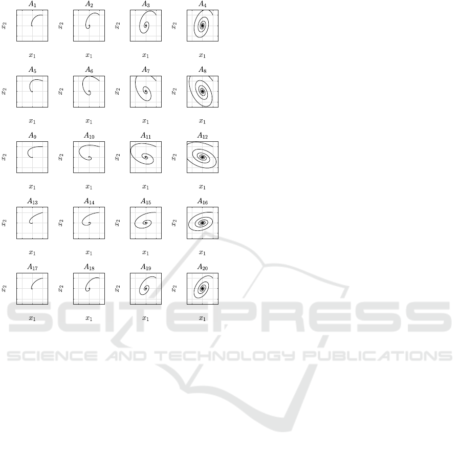
2.2 Planar Systems
We generated twenty linear systems in the plane, con-
structed as follows. We define vectors
θ =

0
9π
40
9π
20
27π
40
9π
10

,
d =

1 2.1544 4.6416 10

,
and the counter-clockwise rotation function
R(θ) =

cos(θ) −sin(θ)
sin(θ) cos(θ)

.
Vector θ is linearly spaced on [0, 0.9π] and d is log-
arithmically, base 10, spaced on [1, 10]. For j =
1, 2, 3, 4, 5 and k = 1, 2, 3, 4, we then define matrices
V
j
=

R(θ
j
)

1
1

R

θ
j
+
π
3


1
1

and E
k
=

−1 −d
k
d
k
−1

.
Finally, we set
A
k+4( j−1)
= V
j
E
k
V
−1
j
(10)
and consider the switched systems (3) with these A
m
and
/
0 ̸= P ⊆ Q = {1, 2, . . . , 20}.
Note that the eigenvalues of A
k+4( j−1)
are λ =
−1±d
k
√
−1 and, thus, the origin is exponentially sta-
ble for each of the linear systems with the same rate
of attraction. The rotation speed, however, is different
for different k. Trajectories for these systems, starting
at (1, 1), are drawn in Fig. 1.
For some subsets
/
0 ̸= P ⊆ Q , the origin is an
exponentially stable equilibrium of the correspond-
ing switched system, for example, for all singe ele-
ment P ; however, for other subsets P the origin is
unstable. The results of our computations are sum-
marised in Table 2. For the reasonable tolerance pa-
rameter ε = 10
−3
, all solvers deliver identical results.
We also tried the (unreasonable) tolerance parameter
ε = 10
−16
that surprisingly delivered more useful so-
lutions for the badly conditioned 5D systems. How-
ever, for the planar systems the results are less inter-
esting. MOSEK and SDPT3 report all LMIs as fea-
sible, however, not simply by reporting P = 0 as a
solution as one might expect for such a low tolerance
and, indeed, do find all 1279 solutions. SeDuMi is un-
affected by the low tolerance and delivers exactly the
Lyapunov Function Computation for Linear Switched Systems: Comparison of SDP and LP Approaches
63

-1 0 1
-1
0
1
-1 0 1
-1
0
1
-1 0 1
-1
0
1
-1 0 1
-1
0
1
-1 0 1
-1
0
1
-1 0 1
-1
0
1
-1 0 1
-1
0
1
-1 0 1
-1
0
1
-1 0 1
-1
0
1
-1 0 1
-1
0
1
-1 0 1
-1
0
1
-1 0 1
-1
0
1
-1 0 1
-1
0
1
-1 0 1
-1
0
1
-1 0 1
-1
0
1
-1 0 1
-1
0
1
-1 0 1
-1
0
1
-1 0 1
-1
0
1
-1 0 1
-1
0
1
-1 0 1
-1
0
1
Figure 1: Trajectories of the systems
˙
x = A
m
x, m =
1, 2, . . . , 20, starting at (1, 1). The matrices A
m
are defined
in (10).
same results as with ε = 10
−3
. One way to interpret
these results, together with the results for the badly
conditioned 5D-systems, is that one should use a tol-
erance that seems unreasonably low, like ε = 10
−16
,
and then verify the reported solutions. Spotting the
false positives is computationally very cheap and one
might get solutions that are missed with a seemingly
more reasonable tolerance parameter.
3 NUMERICAL STUDY:
COMPARING LP AND SDP
As discussed in the introduction, the switched linear
system (3) with an exponentially stable equilibrium
at the origin does not necessarily possess a QCLF.
To investigate how limiting QCLFs are in practice,
we compared the results from the last section for the
planar systems with the LP approach from (Andersen
et al., 2023) to search for a common piecewise lin-
ear Lyapunov function. The LP problems were solved
using Gurobi (Gurobi Optimization, LLC, 2023). At
least in theory, there always exists a piecewise linear
Lyapunov function for the system (3), if the origin is
exponentially stable, cf. (Goebel et al., 2006; Mason
et al., 2006; Mason et al., 2022). Thus a priori, we ex-
pected that the LP approach will be able to compute
CLFs for more subsets P ⊆ Q = {1, 2, . . . , 20} than
the LMI approach.
Table 3 compares the performance between the
two approaches. As we can see for |P | > 1, the LP
approach is always able to generate more common
piecewise linear Lyapunov function than the SDP ap-
proach and the difference is larger, the more elements
P has. Indeed, for |P | = 2, the SDP approach can af-
firm the stability of 75% of the systems that the LP
approach successfully asserts as stable, but this ratio
decreases to 50% for |P | = 3 and 33% for |P | = 4;
for |P | = 8, the ratio is down to 2% and, for systems
with |P | > 8, the SDP approach is not able to affirm
the stability of any system.
Comparing the approaches with three-
dimensional systems form the appendix we get
similar results (see Table 4).
4 PRECONDITIONING FOR THE
LP APPROACH
In the LP approach from (Andersen et al., 2023), to
search for a piecewise linear CLF for the switched
linear system (3), a neighbourhood of the origin must
first be triangulated. Then a LP is created, whose vari-
ables are the values of the piecewise linear CLF to be
parametrised for the system. The number of the con-
straints of the LP problem is the number of simplices
in the triangulation times the dimension. The vertices
of the simplices of the triangulation are put on the in-
teger grid z ∈ Z
n
, ∥z∥
∞
= K, where K ∈ N is a pa-
rameter that determines the resolution, or fineness, of
the triangulation. The triangulation with resolution
parameter K is denoted T
K
. To count the total num-
ber of simplices in the triangulation T
K
for a given
dimension n, note that ∥z∥
∞
= K has 2
n
sides. To see
this, note that by fixing one component z
i
of z to K
or −K we have fixed the side. Since z has n compo-
nents, there are 2
n
ways to do this. Each side then
has (2K)
n−1
hypercubes of dimension n −1 and each
hypercube leads to (n −1)! different simplices. Thus,
the number of simplices as a function of dimension n
and resolution parameter K is given by
Number of simplices = 2
n
(2K)
n−1
(n −1)!.
We can see that the number of simplices grows very
fast with the dimension (curse of dimensionality).
For a more visual image of the number of simplices
needed, see Table 5.
SIMULTECH 2023 - 13th International Conference on Simulation and Modeling Methodologies, Technologies and Applications
64

Table 2: Overview of 2D results. PT: Solution reported and passed test, FP: False positive (solution reported but did not
pass test), I: Infeasible, and T: Total number of LMIs problems. The tolerance parameter ε = 10
−3
appears reasonable and
ε = 10
−16
does not. Note the effect of the simplification of not considering supersets of a set P , for which the LMI problem
is infeasible. With ε = 10
−3
only 1,366 LMIs have to be solved instead of 2
20
−1 = 1, 047, 296, i.e. for every subsets P ̸=
/
0
of Q .
Solver ε PT FP I T
MOSEK
10
−3
1279 0 87 1366
SDPT3 1279 0 87 1366
SeDuMi 1279 0 87 1366
MOSEK
10
−16
1279 1,047,296 0 1,048,575
SDPT3 1279 1,047,296 0 1,048,575
SeDuMi 1279 0 87 1366
Table 3: Ratio, in percentage, of the two-dimensional problems from Section 2.2 successfully solved using SDP to problems
successfully solved using LP.
# of matrices # sys. solved using SDP # sys. solved using LP SDP / LP LP / tot. total # of sys.
1 20 20 100% 100% 20
2 104 142 73.24% 74.74% 190
3 260 522 49.81% 45.79% 1, 140
4 370 1092 33.88% 22.54% 4, 845
5 316 1458 21.67% 9.404% 15, 504
6 160 1261 12.69% 3.253% 38, 760
7 44 696 6.322% 0.8978% 77,520
8 5 233 2.146% 0.1850% 125, 970
9 0 42 0% 0.02501% 167,960
10 0 3 0% 0.001624% 184, 756
11 0 0 ⋆ 0% 167, 960
If the LP approach from (Andersen et al., 2023)
is to be applicable in dimensions larger than n = 3
or n = 4, then some reduction in the number of sim-
plices is clearly needed. A promising preconditioning
approach was presented in (Andersen et al., 2023).
The idea is to make a coordinate transform such
that V(x) = ∥x∥
2
is closer to fulfilling the conditions
of a Lyapunov function. To compute such a coordi-
nate transform we first solve the Lyapunov equation
A
T
m
P
m
+ P
m
A
m
= −I
n
∀m ∈ P .
Since the individual subsystems
˙
x = A
m
x have an ex-
ponentially stable equilibrium at the origin, the ma-
trices A
m
are Hurwitz and these equations all have
a positive definite solution P
m
≻ 0. Thus, for each
subsystem
˙
x = A
m
x, the function V
m
(x) = x
T
P
m
x is
a quadratic Lyapunov function. We then define the
matrix
R :=
∑
m∈P
λ
m
P
m
as a convex combination of the P
m
, that is, λ
m
≥ 0 for
all m ∈ P and
∑
m∈P
λ
m
= 1.
Next, we use the coordinate transform x 7→
R
1
2
x; that is, we replace the matrices A
m
by
e
A
m
:=
R
1
2
A
m
R
−
1
2
. We call this procedure preconditioning of
the switched system (3). Note that if |P | = 1 then
V (x) =
p
x
T
I
n
x = ∥x∥
2
is a Lyapunov function for
the transformed system. In Figure 2 we show how
trajectories of two systems are altered through pre-
conditioning the switched system.
In many cases, one can compute a piecewise lin-
ear CLF for switched system (3) with fewer simplices,
that is, with a lower K in the triangulation T
K
. How-
ever, it is not transparent how to choose the λ
m
in the
convex combination. In Fig. 3, we investigate this for
two examples from the three-dimensional linear sys-
tems outlined in the appendix. In both cases, we con-
sider two systems,
˙
x = A
r
x and
˙
x = A
s
x, the coordi-
nate transform
R
λ
= λP
r
+ (1 −λ)P
s
,
which corresponds to λ
r
= λ and λ
s
= 1 −λ, and re-
port the lowest resolution parameter K, for which we
could compute a piecewise linear CLF for the system.
For r = 6 and s = 9, we see the typical case: Pre-
conditioning allows us to compute a Lyapunov func-
tion using considerably fewer simplices. However,
there are also cases, where preconditioning is not of
advantage or where it is even counterproductive, as it
is for r = 3 and s = 12, shown in the lower panel of
Fig. 3. However, usually the preconditioning has the
Lyapunov Function Computation for Linear Switched Systems: Comparison of SDP and LP Approaches
65

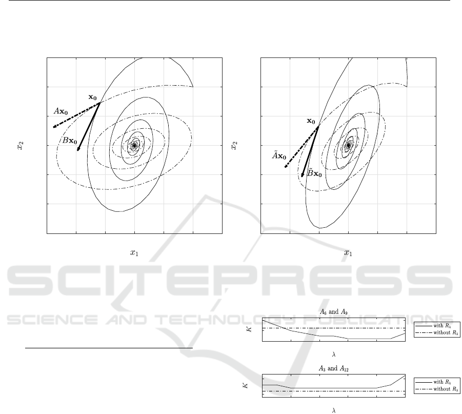
Table 4: Ratio, in percentage, of the three-dimensional problems from the Appendix successfully solved using SDP to prob-
lems successfully solved using LP.
# of matrices # sys. solved using SDP # sys. solved using LP SDP / LP LP / tot. total # of sys.
1 12 12 100% 100% 12
2 9 10 90% 15.15% 66
3 1 3 33.33% 1.36% 220
4 0 0 ⋆ 0 495
-1.5 -1 -0.5 0 0.5 1 1.5
-1.5
-1
-0.5
0
0.5
1
1.5
(a) Angle is 37.11
◦
.
-1.5 -1 -0.5 0 0.5 1 1.5
-1.5
-1
-0.5
0
0.5
1
1.5
(b) Angle is now 20.97
◦
.
Figure 2: Exemplary angle between vector fields x 7→ Ax and x 7→Bx (a) and the transformed (or preconditioned) vector fields
x 7→
˜
Ax and x 7→
˜
Bx (b) at a point x
0
.
Table 5: Some examples of the number of simplices in the
triangulation T
K
in different dimensions n.
n K Number of simplices in T
K
2 5 40
2 10 80
2 50 400
2 100 800
3 5 1,600
3 10 6,400
3 50 160,000
3 100 640,000
4 5 96,000
4 10 768,000
4 50 96,000,000
4 100 768,000,000
5 5 7,680,000
5 10 122,880,000
5 50 7.68 ·10
10
5 100 1.2288 ·10
12
effect of reducing the number of simplices needed,
but how to chose the optimal parameter λ remains an
open problem. Note that this problem is of much prac-
tical value for systems of higher dimensions, where
the number of simplices possible in the LP is the lim-
0 0.2 0.4 0.6 0.8 1
20
40
60
0 0.2 0.4 0.6 0.8 1
50
100
Figure 3: Lowest resolution factor K that delivers a piece-
wise linear CLF as a function of λ for two example sets
for three-dimensional systems. The number of simplices
needed is 64K
2
. While 64 ·45
2
= 129, 600 simplices are
needed without preconditioning, we get a solution with
64 ·25
2
= 40, 000 simplices for λ ∈[0.6, 0.9] for P = {6, 9}
(upper figure). For P = {3, 12}, we have the untypical case
that the preconditioning is counterproductive (lower figure).
The first example possesses a QCLF while the second does
not.
iting factor. Understanding what effect the precon-
ditioning of the systems has, is one of the main rea-
sons for developing the app AngleAnalysis discussed
in the next section.
SIMULTECH 2023 - 13th International Conference on Simulation and Modeling Methodologies, Technologies and Applications
66

5 THE AngleAnalysis APP
As known from the literature and seen in the pre-
ceding sections, the stability of the origin of (3) for
a given set of matrices, is far from transparent. To
better visualise the problem for two given matrices
A, B ∈ R
n×n
, n = 2, 3, we developed the application
AngleAnalysis, which visualises the angles given by
∠(Ax, Bx) := arccos

⟨
Ax, Bx
⟩
∥Ax∥∥Bx∥

between vector fields x 7→ Ax and x 7→ Bx (see Fig. 2
(a)).
In the following, we explain in some detail how
this angle relates to the stability of the origin, which
is equivalent to the existence of a CLF for the sys-
tems
˙
x = Ax and
˙
x = Bx. Consider (3) and the def-
inition of a Lyapunov function. Lyapunov function
V : R
n
→R
+
is such that V (
¯
x) = 0 if and only if
¯
x = 0
is an equilibrium point, and the directional derivative
along any system trajectory is strictly negative; that
is,
⟨
∇V (x), A
m
x
⟩
< 0 for all m ∈ P and x ̸= 0.
Intuitively, since a CLF must fulfil
⟨
∇V (x), Ax
⟩
<
0 and
⟨
∇V (x), Bx
⟩
< 0, that is, ∠(∇V (x), Ax) > 90
◦
and ∠(∇V(x), Bx) > 90
◦
, for all x ̸= 0, this condition
is more difficult to satisfy for vector fields x 7→ Ax
and x 7→ Bx if ∠(Ax, Bx) tends to be large. In other
words, the smaller the angle between Ax and Bx for
a particular x ∈ R
n
, the more “space” there is to put
the gradient ∇V (x), and it should be easier to con-
struct a function V : R
n
→ [0, ∞), whose gradient ful-
fills ∠(∇V (x), Ax) > 90
◦
and ∠(∇V (x), Bx) > 90
◦
,
for all x ̸= 0.
It is also helpful to look at the two extreme cases,
when there is a point
ˆ
x ∈ R
n
, for which the angle be-
tween A
ˆ
x and B
ˆ
x is 180
◦
, and when the angle is 0
◦
for
all x ∈ R
n
. In the former case, there exists a constant
c > 0 such that A
ˆ
x = −cB
ˆ
x, and a Lyapunov function
V such that
⟨
∇V (x), Ax
⟩
< 0 and
⟨
∇V (x), Bx
⟩
< 0
cannot exists, since assuming that there is one leads
to the following contradiction:
⟨
∇V (x), Ax
⟩
=
⟨
∇V (x), −cBx
⟩
= −c
⟨
∇V (x), Bx
⟩
.
Hence, there cannot exist a CLF for the systems
˙
x = Ax and
˙
x = Bx. In the other extreme case, if
∠(Ax, Bx) = 0
◦
for all x ∈ R
n
then every Lyapunov
function for
˙
x = Ax is a Lyapunov function for
˙
x = Bx
and vice versa.
The AngleAnalysis app takes in any two matri-
ces A ∈ R
n×n
and B ∈ R
n×n
and visualises the angle
(a) (b)
Figure 4: Angle visualisation for matrices from (Andersen
et al., 2023) with a = 0.1 and b = 13.25 (a) without pre-
conditioning, (b) with λ
a
= 0.2 and λ
b
= 0.8. A piecewise
linear CLF was obtained for the preconditioned system us-
ing a much lower resolution K than without.
Table 6: Maximum, minimum, mean and standard devia-
tion of the angles between the trajectories of A
6
and A
9
at
(x, y, z) ∈ [−1, 1]
3
where x = x
1
, y = x
2
and z = x
3
are 30
points, evenly spaced on the interval.
λ
6
λ
9
Max Min Mean Std K
N/A N/A 176.0 2.97 77.5 43.0 45
0.7 0.3 176.5 1.02 105.3 30.4 25
0 1 176.8 0.83 82.5 37.7 60
∠(Ax, Bx) through a heat-map, where dark colors in-
dicate small angles and bright colors indicate large an-
gles. For n = 2, the heat-map is plotted in the square
[−1, 1]
2
. For n = 3, the heat-map is plotted in the
square [−1, 1]
2
×{z}, where the parameter z = x
3
can
be continuously varied in the interval [−1, 1].
As discussed in Section 4, effect of the precondi-
tioning on the LP problem is not intuitive. For some
systems, for example the ones in (Andersen et al.,
2023), the app gives clear indication of whether one
can expect a reduction in the number of simplices, see
Figure 4. However, in other cases the stability prop-
erties or preconditioning benefits are not transparent.
Figures 5 and 6 show the angle heat map without pre-
conditioning and with two different preconditionings.
The resulting angle statistics can be found in tables 6
and 7. In neither case the app gives a clear indica-
tion of whether one can expect stability under arbi-
trary switching. The reason is that even though it is
locally not difficult to put gradients ∇V (x) that fulfil
∠(∇V (x), Ax) > 90
◦
and ∠(∇V (x), Bx) > 90
◦
, then
V : R
n
→ [0, ∞) has to be a continuous function on
R
n
, and the problem of the existence of a CLF is a
highly non-local one.
Table 7: Maximum, minimum, mean and standard devia-
tion of the angles between the trajectories of A
3
and A
12
at
(x, y, z) ∈ [−1, 1]
3
where x = x
1
, y = x
2
and z = x
3
are 30
points, evenly spaced on the interval.
λ
3
λ
12
Max Min Mean Std K
N/A N/A 143.0 1.04 74.2 25.2 60
0.7 0.3 136.3 1.14 70.0 20.0 70
1 0 151.9 1.38 64.2 23.0 110
Lyapunov Function Computation for Linear Switched Systems: Comparison of SDP and LP Approaches
67

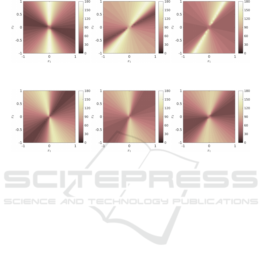
(a) (b) (c)
Figure 5: Angle visualisation for A
3
and A
12
at z = 0. (a) Without preconditioning, (b) with λ
6
= 0.7 and λ
9
= 0.3, (c) with
λ
6
= 0 and λ
9
= 1. Corresponding angle data can be found in Table 6.
(a) (b) (c)
Figure 6: Angle visualisation for A
3
and A
12
at z = 0. (a) Without preconditioning, (b) with λ
3
= 0.7 and λ
12
= 0.3, (c) with
λ
3
= 1 and λ
12
= 0. Corresponding angle data can be found in Table 7.
6 CONCLUSIONS
We compared different semidefinite programming
(SDP) solvers for computing quadratic common Lya-
punov functions (QCLFs) for a variety of switched
linear systems. In particular we tried different param-
eters ε > 0 to force positive definiteness A ≻0 through
A ⪰ εI
n
and got the somewhat surprising results that
very small ε performed better in some examples. We
compared QCLF to piecewise linear CLF computed
by solving linear programming (LP) problems. As
expected the LP approach is able to assert stability
for more switched systems than the SDP approach.
The disadvantage of the LP approach is that a trian-
gulation of the state-space is needed, which results
in a very high number of simplices in higher dimen-
sions. To leverage this problem a certain precondi-
tioning of the systems has been suggested. However,
how to chose the parameters of the preconditioning is
far from transparent. We developed the app Angle-
Analysis to get visual information about the effect of
the preconditioning and gave examples of its use.
In summary, we presented state-of-the art ap-
proaches to determine the stability of switched sys-
tems. While the SDP approach is faster, it solves the
problem far less often than the more time-intensive
approach using LP. As mentioned in the introduction,
extending the SDP approach to higher-order polyno-
mial Lyapunov functions seems promising, as it is
less conservative. Finally, as shown in this paper
preconditioning greatly accelerates the LP approach.
Thus, in the future, we will continue investigating ef-
ficient methods for obtaining suitable precondition-
ing, in particular, for switched systems of higher or-
der.
ACKNOWLEDGEMENTS
Submitted 03/15/2023. This work was supported
in part by the Icelandic Research Fund under Grant
228725-051 and has received funding from European
Union’s Horizon 2020 research and innovation pro-
gramme under grant agreement no. 965417.
REFERENCES
Agrachev, A. and Liberzon, D. (2001). Lie-algebraic sta-
bility criteria for switched systems. SIAM J. Control
Optim., 40(1):253–269.
SIMULTECH 2023 - 13th International Conference on Simulation and Modeling Methodologies, Technologies and Applications
68

Andersen, S., Giesl, P., and Hafstein, S. (2023). Common
Lyapunov functions for switched linear systems: Lin-
ear programming-based approach. IEEE Control Sys-
tems Letters, 7:901–906.
Aubin, J.-P. and Cellina, A. (1984). Differential Inclusions.
Springer.
Bakhshande, F., Bach, R., and S
¨
offker, D. (2020). Ro-
bust control of a hydraulic cylinder using an observer-
based sliding mode control: Theoretical development
and experimental validation. Control Engineering
Practice, 95:104272.
Blanchini, F. (1995). Nonquadratic Lyapunov functions for
robust control. Automatica, 31(3):451–461.
Blanchini, F. and Carabelli, S. (1994). Robust stabiliza-
tion via computer-generated Lyapunov functions: an
application to a magnetic levitation system. In Pro-
ceedings of the 33th IEEE Conference on Decision
and Control, volume 2, pages 1105–1106.
Blanchini, F. and Miani, S. (2008). Set-theoretic methods in
control. Systems & Control: Foundations & Applica-
tions. Birkh
¨
auser.
Boyd, S., El Ghaoui, L., Feron, E., and Balakrishnan,
V. (1994). Linear matrix inequalities in system and
control theory, volume 15 of SIAM Studies in Ap-
plied Mathematics. Society for Industrial and Applied
Mathematics (SIAM), Philadelphia, PA.
Brayton, R. and Tong, C. (1979). Stability of dynamical
systems: A constructive approach. IEEE Trans. Cir-
cuits and Systems, 26(4):224–234.
Brayton, R. and Tong, C. (1980). Constructive stability
and asymptotic stability of dynamical systems. IEEE
Trans. Circuits and Systems, 27(11):1121–1130.
Clarke, F. (1990). Optimization and Nonsmooth Analysis.
Classics in Applied Mathematics. SIAM.
Cohen, N. and Lewkowicz, I. (1993). A necessary and suf-
ficient criterion for the stability of a convex set of ma-
trices. IEEE Trans. Automat. Control, 38(4):611–615.
Giesl, P. and Hafstein, S. (2015). Review of computational
methods for Lyapunov functions. Discrete Contin.
Dyn. Syst. Ser. B, 20(8):2291–2331.
Goebel, R., Hu, T., and Teel, A. (2006). Current Trends
in Nonlinear Systems and Control. Systems and Con-
trol: Foundations & Applications, chapter Dual Ma-
trix Inequalities in Stability and Performance Analy-
sis of Linear Differential/Difference Inclusions, pages
103–122. Birkhauser.
Goebel, R., Sanfelice, R., and Teel, A. (2012). Hybrid Dy-
namical Systems. Princeton University Press.
Gr
¨
une, L. and Junge, O. (2016). Gew
¨
ohnliche Differential-
gleichungen. Springer, Wiesbaden, 2nd edition.
Gurobi Optimization, LLC (2023). Gurobi Optimizer Ref-
erence Manual.
Khalil, H. (2002). Nonlinear Systems. Pearson, 3. edition.
Liberzon, D. (2003). Switching in systems and control.
Systems & Control: Foundations & Applications.
Birkh
¨
auser.
L
¨
ofberg, J. (2004). YALMIP: A toolbox for modeling and
optimization in MATLAB. In In Proceedings of the
CACSD Conference, Taipei, Taiwan.
Mason, P., Boscain, U., and Chitour, Y. (2006). Common
polynomial Lyapunov functions for linear switched
systems. SIAM J. Control Optim., 45(1):226–245.
Mason, P., Chitour, T., and Sigalotti, M. (2022). On univer-
sal classes of Lyapunov functions for linear switched
systems. arXiv:2208.09179.
MATLAB (2022). 9.12.0.2039608 (R2022a) Update 5. The
MathWorks Inc., Natick, Massachusetts.
Molchanov, A. and Pyatnitskiy, E. (1986). Lyapunov func-
tions that specify necessary and sufficient conditions
of absolute stability of nonlinear nonstationary control
systems I, II. Automat. Remote Control, 47:344–354,
443–451.
Molchanov, A. and Pyatnitskiy, E. (1989). Criteria of
asymptotic stability of differential and difference in-
clusions encountered in control theory. Systems Con-
trol Lett., 13(1):59–64.
MOSEK ApS (2019). The MOSEK optimization toolbox for
MATLAB manual. Version 9.0.
Ohta, Y. (2001). On the construction of piecewise lin-
ear Lyapunov functions. In Proceedings of the 40th
IEEE Conference on Decision and Control., volume 3,
pages 2173–2178.
Ohta, Y. and Tsuji, M. (2003). A generalization of piece-
wise linear Lyapunov functions. In Proceedings of the
42nd IEEE Conference on Decision and Control., vol-
ume 5, pages 5091–5096.
Piccini, J., August, E., Hafstein, S., and Andersen, S.
(2023). Stability of switched systems with multiple
steady state solutions. In (submitted).
Polanski, A. (1997). Lyapunov functions construction by
linear programming. IEEE Trans. Automat. Control,
42:1113–1116.
Polanski, A. (2000). On absolute stability analysis by poly-
hedral Lyapunov functions. Automatica, 36:573–578.
Prajna, S. and Papachristodoulou, A. (2003). Analysis
of switched and hybrid systems - beyond piecewise
quadratic methods. In Proceedings of the 2003 Amer-
ican Control Conference, pages 2779–2784.
Sturm, J. (1999). Using SeDuMi 1.02, a MATLAB toolbox
for optimization over symmetric cones. Optimization
Methods and Software, 11–12:625–653. Version 1.05
available from http://fewcal.kub.nl/sturm.
Toh, K. C., Todd, M. J., and T
¨
ut
¨
unc
¨
u, R. H. (1999). Sdpt3 -
a matlab software package for semidefinite program-
ming, version 1.3. Optimization Methods and Soft-
ware, 11(1-4):545–581.
Veer, S. and Poulakakis, I. (2020). Switched systems with
multiple equilibria under disturbances: Boundedness
and practical stability. IEEE Transactions on Auto-
matic Control, 65(6):2371–2386.
Wang, K. and Michel, A. (1996). On the stability of a family
of nonlinear time-varying system. IEEE Trans. Cir-
cuits and Systems, 43(7):517–531.
Yfoulis, C. and Shorten, R. (2004). A numerical technique
for the stability analysis of linear switched systems.
Int. J. Control, 77(11):1019–1039.
Lyapunov Function Computation for Linear Switched Systems: Comparison of SDP and LP Approaches
69

APPENDIX
We generated 12 three-dimensional matrices to exam-
ine the effects of the preconditioning outlined in Sec-
tion 4 with the following MATLAB commands:
Rz = @ ( th )[ c os ( th ), -sin ( th ), 0;
sin ( th ) , cos ( th ), 0;
0, 0, 1];
Ry = @ ( th )[ cos(th ) , 0, sin ( th );
0, 1 , 0;
- sin ( th ) , 0 , co s (th )];
Rx = @ ( th )[1 , 0, 0;
0, cos ( th ) , - sin ( th );
0, sin ( th ) , cos ( th )] ;
m = 3; n = 2; l = 2;
th1 = li ns pace (.9 /m ,0.9 , m)* pi ;
th2 = li ns pace (0 ,0.9 , n)* pi ;
th3 = li ns pace (0 ,0.9 , l)* pi ;
nu m_ sys = m * n * l ;
A_3D = zero s (3 ,3 , nu m _sys );
init = [1 ; 1 ; 1];
E = [ -10 , 0 , 0;
0, -1, 5;
0, -5, -1];
for i = 1: nu m _ s ys
r = c eil ( i /( n * l ));
t = mod ( c eil ( i / l ) -1 , n ) +1;
s = mod ( i -1 , l )+1;
V = [ Rx ( th1 ( r ) )* init , ...
Ry ( t h1 ( r )+ th2 ( t ))* init , ...
Rz ( t h1 ( r )+ th2 ( t )+ th3 ( s ))* init ];
A_3D (: ,: , i ) = V * E / V ;
end
SIMULTECH 2023 - 13th International Conference on Simulation and Modeling Methodologies, Technologies and Applications
70