A Global Multi-Temporal Dataset with STGAN Baseline for Cloud and

Cloud Shadow Removal

Morui Zhu

2 a

, Chang Liu

1, 2 b

and Tam

as Szir

anyi

1, 3 c

Machine Perception Research Laboratory of Institute for Computer Science and Control (SZTAKI), H-1111 Budapest,

Kende u. 13-17, Hungary

Department of Networked Systems and Services, Budapest University of Technology and Economics, BME Informatika

ulet Magyar tud

osok k

utja 2, Budapest, Hungary

Faculty of Transportation Engineering and Vehicle Engineering, Budapest University of Technology and Economics

(BME-KJK), M

uegyetem rkp. 3., Budapest, H-1111, Hungary

Keywords:

Cloud and Cloud Shadow Removal, Generative Adversarial Networks, Spatio-Temporal, Sentinel-2.

Abstract:

Due to the inevitable contamination of thick clouds and their shadows, satellite images are greatly affected,

which signiﬁcantly reduces the usability of data from satellite images. Therefore, obtaining high-quality image

data without cloud contamination in a speciﬁc area and at the time we need it is an important issue. To address

this problem, we collected a new multi-temporal dataset covering the entire globe, which is used to remove

clouds and their shadows. Since generative adversarial networks (GANs) perform well in conditional image

synthesis challenges, we utilized a spatial-temporal GAN (STGAN) to eliminate clouds and their shadows in

optical satellite images. As a baseline model, STGAN demonstrated outstanding performance in peak signal-

to-noise ratio (PSNR) and structural similarity index (SSIM), achieving scores of 33.4 and 0.929, respectively.

The cloud-free images generated in this work have signiﬁcant utility for various downstream applications in

real-world environments. Dataset is publicly available: https://github.com/zhumorui/SMT-CR

1 INTRODUCTION

Cloud and cloud shadow broadly exist in remotely

sensed images(Sudmanns et al., 2020), which limit

the downstream applications relying on optical re-

motely sensed imagery including environmental mon-

itoring(Gure et al., 2009), urban planning(Matwin

et al., 2017), land cover classiﬁcation(Kussul et al.,

2017)(Garnot and Landrieu, 2021)(Wurm et al.,

2019), etc. Cloud is generated by vast ﬂoating water

droplets, and cloud shadow is formed by optical linear

propagation covering. Therefore, authentic reﬂectiv-

ity information is destroyed within the covered areas.

According to the survey research(Mao et al., 2019),

global cloud cover reaches up to 66%. Many existing

applications rely on clear images, while those that are

polluted with clouds are often excluded. Cloud and

cloud shadow removal of RS images can signiﬁcantly

improve the utilization of RS data. Over the past few

decades, numerous methods have been proposed to

https://orcid.org/0000-0002-5820-1441

https://orcid.org/0000-0001-6610-5348

https://orcid.org/0000-0003-2989-0214

address the challenge of thick cloud removal from RS

images. Unfortunately, however, there are not sufﬁ-

cient such baseline datasets and baselines to evaluate

so far. A multi-temporal baseline dataset for cloud re-

moval tasks should meet the following requirements:

1) The dataset should encompass a large number

of samples with global coverage, spanning diverse en-

vironmental conditions such as deserts, oceans, and

lands.

2) To minimize changes in the same geographical

area between remotely sensed (RS) images captured

at different times, the maximum time interval between

RS images should preferably not exceed one month.

3) Real cloudy images often exhibit complex

shape and color compositions, including cloud shad-

ows, which necessitate the use of an accurate cloud

and cloud shadow mask for RS images.

4) Given the variations in cloud cover and other

factors, each sample in the dataset presents a unique

level of difﬁculty for cloud removal. Therefore, it is

necessary to classify the samples into different levels

of difﬁculty to accurately evaluate the performance of

the model. To ensure that the dataset encompasses a

206

Zhu, M., Liu, C. and Szirányi, T.

A Global Multi-Temporal Dataset with STGAN Baseline for Cloud and Cloud Shadow Removal.

DOI: 10.5220/0012039600003497

In Proceedings of the 3rd International Conference on Image Processing and Vision Engineering (IMPROVE 2023), pages 206-212

ISBN: 978-989-758-642-2; ISSN: 2795-4943

 2023 by SCITEPRESS – Science and Technology Publications, Lda. Under CC license (CC BY-NC-ND 4.0)

diverse range of difﬁculties, it is important to include

samples spanning the full spectrum from easy to hard.

Traditional methods for cloud removal, such as

mean and median ﬁlters, have been widely em-

ployed to ﬁll in missing regions of multi-temporal

remote sensing images (Helmer and Ruefenacht,

2005)(Ramoino et al., 2017)(Tseng et al., 2008).

However, these methods typically require a large

number of clear images, which may not always be

available. (Ramoino et al., 2017) utilized Sentinel-2

images spanning a period of three months, while the

changes may occur in this long time interval. (Cheng

et al., 2014) uses Markov Random Fields to leverage

spatial and temporal information, the process of ﬁnd-

ing similar pixels and estimating the cloud-free values

can be time-consuming, and the MRF model requires

signiﬁcant computational resources for optimization.

Another solution is to use fusion Markov Random

Field optimization for multispectral and multitem-

poral image series (Szir

anyi and Shadaydeh, 2013),

where instead of learning on differently located im-

age data, the same image position is applied but with

different color bandwidth and time-instant data. If we

do not have historical data about a region, then similar

cases should be found to train a deep learning solution

based on other region instances. In a recent study,

(Zhang et al., 2020) introduced a novel approach

utilizing Convolutional Neural Networks (CNNs) to

address the issue of missing data regions in multi-

temporal images. However, the method highly de-

pends on data, and it cannot reconstruct missing re-

gions without auxiliary temporal information.

Compared to previous methods, generative mod-

els show state-of-art performance while dealing with

image translation(Isola et al., 2017)(Zhu et al.,

2017)(Hettiarachchi et al., 2021)(Sharma et al.,

2019). (Sarukkai et al., 2019) use spatio-temporal

Generative Adversarial Networks to remove clouds

for cloudy image pairs. In order to achieve the desired

level of accuracy and learn the information from other

temporal images, it requires 3 multi-temporal cloudy

images with infrared images. However, large areas in

multi-temporal images are obscured by cloud cover,

which is not ideal for GANs to reconstruct accurate

and real information in training and predicting peri-

ods. To accurately evaluate the performance of mod-

els for cloud removal tasks, we create an enhanced

new dataset from sentinel-2 RS images for cloud and

cloud shadow removal tasks. The main objective

of this work is to construct a larger spatio-temporal

dataset for cloud removal and cloud shadow removal

tasks from satellite images. This dataset is collected

and constructed under speciﬁc requirements, cover-

ing global areas with various scenes such as deserts,

oceans, and lands. The time interval between any

spatio-temporal data of the same region does not ex-

ceed one month to prevent changes in the same loca-

tion. The dataset has accurate semantic segmentation

of clouds and shadows and is divided into different

levels of difﬁculty based on the tasks. The dataset

includes data on various difﬁculties as much as possi-

ble.

In the next few sections, Section 2 presents the

dataset collection and cleaning, including the prob-

lem deﬁnition and cloud detection. In Section 3, the

STGAN strategies and the experiment results are pre-

sented, followed by the evaluation, along with a de-

scription of the relevant models and training and sys-

tem information. Conclusions and future work are

drawn in Section 4.

2 DATASETS COLLECTION AND

CONSTRUCTION

2.1 Problem Deﬁnition

We deﬁne χ = R

w×h×C

as the set of multi-spectral

satellite images of size (w, h) = 256 × 256 and C = 4

channels (bands). Let



, Z



t,l

be a collection of

random variables X

, Z

. X

, Z

∈ χ, which represent

a pair of the clear and cloudy image at location l and

time t = 0, 1, . . . . These variables have a joint underly-

ing probability distribution p(



, Z



t,l

), which de-

scribes on-the-ground changes over time and the rela-

tionship between clear and cloudy images.

We assume that X

changes slowly only over time,

i.e., X

≈ X

t−1

, ∀t, ∀l. The effect of cloud cover is the

same over time and at different locations. Our ob-

jective is to learn a model of the conditional distribu-

tion P(X

, . . . , Z

t−T

), T = 2 in our dataset. How-

ever, the major challenge in such a case is that X

and Z

never both exist, ∀t, ∀l, which makes learning

P(X

) difﬁcult.

2.2 Collecting Data From All Over the

World

The dataset consists of two versions: the ﬁrst version

contains original full images with a resolution of 10m

and 10980x10980 pixels per image, while the second

version consists of cropped images of size 256x256.

The construction process of the improved dataset is

illustrated in Figure 1.

To carry out standard preprocessing, we primarily

rely on Level-1C Sentinel-2A/B satellites. The

granules, also known as tiles, are 100x100 km2

A Global Multi-Temporal Dataset with STGAN Baseline for Cloud and Cloud Shadow Removal

207

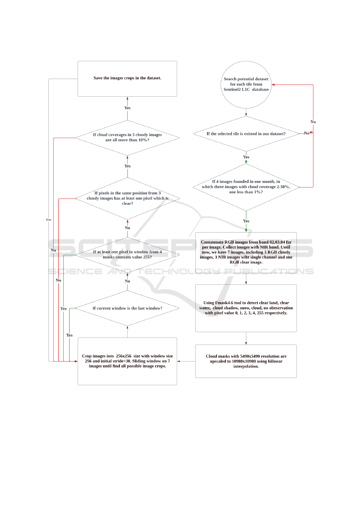
Figure 1: Dataset Construction Pipeline.

ortho-images in the UTM/WGS84 projection. The

European Space Agency provides a sentinel2 tiling

grid ﬁle in KML format, which can be accessed via

the ofﬁcial description available at the following link:

https://sentinel.esa.int/web/sentinel/missions/sentinel-

2/data-products. We utilize the global land mask

tool to verify if the central latitude/longitude of a tile

represents land or sea, as we main aim to eliminate

clouds from land images that contain more activity

information. The geographical distribution of all land

IMPROVE 2023 - 3rd International Conference on Image Processing and Vision Engineering

208

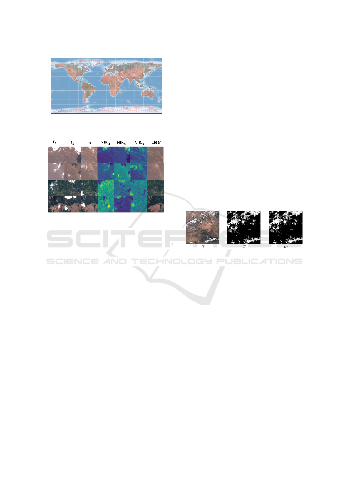
Figure 2: Distribution of all tiles on the land in the world

map.

Figure 3: Examples from data sets, images from left to right

are temporal cloudy images pairs with t

, t

, and t

sensing

time, heatmap of infrared images NIR

, NIR

and NIR

clear images.

tiles is presented in Figure 2.

The present study incorporates band concatena-

tion of RGB and IR channels to exploit their comple-

mentary information. Speciﬁcally, we employ four

bands: B02, B03, B04, and B08, which have a 10m

resolution in the Sentinel2 L1C-level images. The

TCI image is composed of RGB channels with bands

02, 03, and 04. As for the B08 image, it contains

only one channel, which we concatenate into the RGB

images from the three multi-temporal images. More-

over, we convert the 16-bit images into 8 uint format

with pixel values ranging from 0 to 255. Figure 3 il-

lustrates some examples from the ﬁnal dataset.

2.3 Cloud Detection

To train and evaluate our model effectively, we need

to establish certain limitations to ensure the quality of

the RS images. One such limitation is to set a lower

bound on the percentage of cloud coverage in each

image. In order to achieve this, we use cloud masks

that guides us in selecting images with a threshold on

the cloud and cloud shadow coverage percentage. To

obtain precise evaluation results, we select only those

images with a cloud coverage percentage greater than

10%. This lower bound ensures that the task is more

challenging and prevents an increase in accuracy that

is deceptive and does not fairly evaluate the model. In

addition, the cloud coverage percentage in real clear

images should be no more than 1%.

To detect clouds, cloud shadows, snow, water, and

null regions, we use the Fmask4.6(Zhu and Wood-

cock, 2012) tool, which is available at the follow-

ing link: https://github.com/GERSL/Fmask. How-

ever, due to the imprecise boundary of cloud shad-

ows, we perform a dilation operation to improve the

accuracy of the assessment. Speciﬁcally, we dilate the

cloud shadow mask by three pixels to achieve a bet-

ter estimation of coverage, while no dilation is per-

formed for clouds, snow, or water. The original out-

put cloud mask size is 5490x5490, but to match the

10m resolution of sentinel images, we use the bilin-

ear interpolation method to upscale the mask’s size to

10980x10980.

Figure 4 presents a comparison of the cloud and

cloud shadow masks obtained using the Fmask4.6

tool. From comparison, it is evident that the differ-

ence between the two masks is acceptable for further

tasks.

Figure 4: (1) is a cloudy image with an image size

10980x10980. (2) is the original output from the Fmask

tool which is up-scaled into (3) with an image size equal to

10980x10980.

2.4 Multi-Temporal Land Cover Levels

Spatio-temporal models learn the conditional proba-

bility P(X

, . . . , Z

t−T

), T = 2. If a particular re-

gion in an image is occluded, the model can utilize

information from other temporal images in which the

same region is clear. The difﬁculty of each sam-

ple is different depending on the multi-temporal land

cover. We deﬁne L

is the set of land pixels in Z

, and

∪t

= L

∪ L

represent the multi-temporal

land cover. L has a signiﬁcant impact on task dif-

ﬁculty, with a higher value of L resulting in tasks

that are easier to perform. We classify images in our

dataset into different multi-temporal land cover levels

from 0-100, ﬁgure 5 shows the distribution of multi-

temporal land cover levels.

A Global Multi-Temporal Dataset with STGAN Baseline for Cloud and Cloud Shadow Removal

209

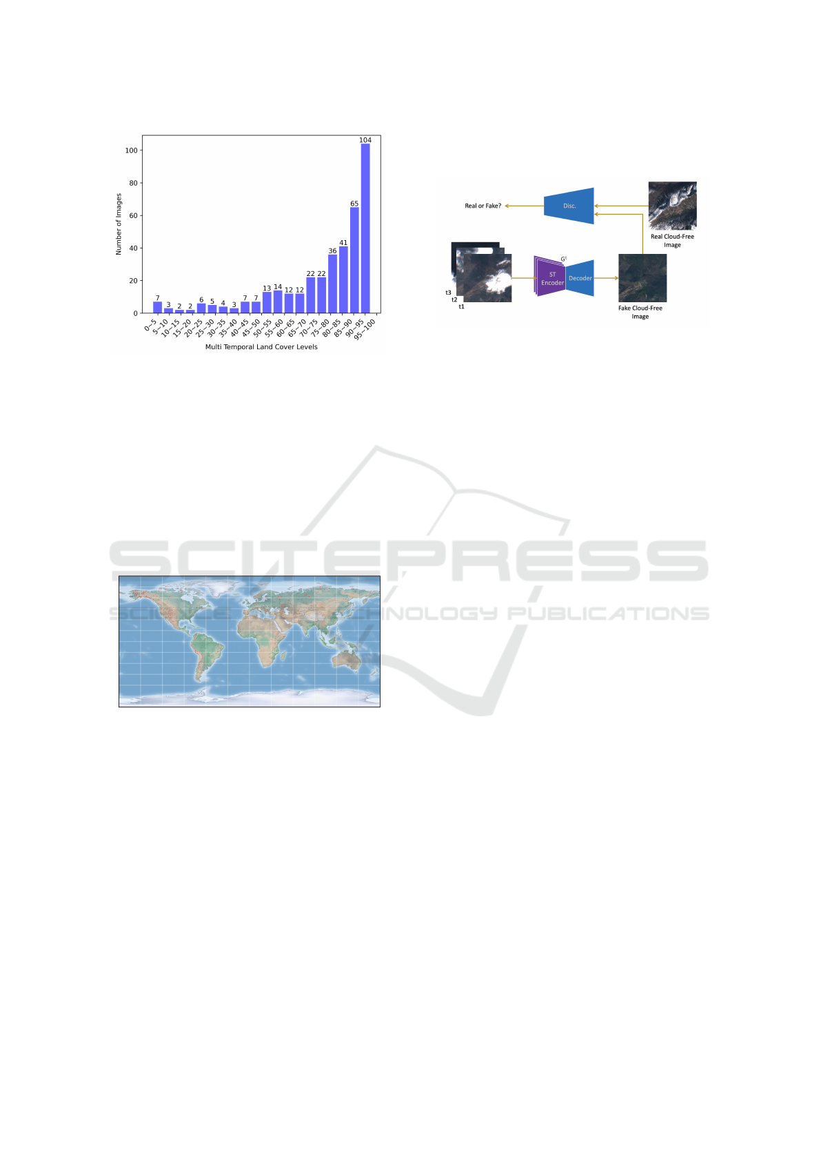
Figure 5: Distribution of multi-temporal land cover levels.

2.5 Cropped Images Dataset from

Diverse Regions

In addition to the original dataset with ultra-high res-

olution, we collected 57474 image crops with size

256x256 from 294 regions around the world for the

purposes of training and evaluating. The distribution

of the collected image pairs can be seen in Figure 6,

which shows the geographical locations of the images

on a world map.

Figure 6: Distribution of the collected image pairs in the

world map.

3 EXPERIMENT RESULTS WITH

STGAN

3.1 STGAN

The process of removing clouds and cloud shadows

from an image can be conceptualized as an image-

to-image translation problem, for which Pix2pix(Isola

et al., 2017) is a versatile conditional adversarial net-

work commonly employed in various image transla-

tion domains. To address this task, we have opted

for STGAN (Sarukkai et al., 2019), an extension of

Pix2pix that supports multiple input channels. In

Figure 7, we present the fundamental architecture of

STGAN.

Figure 7: The fundamental architecture of STGAN, in with

multiple Encoder-Decoder modules support multi-temporal

images as input.

Typically, the model training process on the

dataset requires 24 days using two Nvidia RTX3090

GPUs. Because model training is time-consuming on

the entire dataset, we randomly sample 2572 image

crops to create a subset of the data.

3.2 Hyper Parameters Setup

In contrast to a normal GAN discriminator, which

maps a 256x256 image to a single scalar output, a

PatchGAN maps a 256x256 image to an NxN array.

Latter requires fewer parameters and can handle im-

ages of arbitrary sizes. The Table 1 shows hyperpa-

rameters settings.

GANs with a conditional architecture are capable

of learning a function that maps from an observed im-

age x and a random noise vector z to an output y. This

function can be represented as G: x, z → y.

The objective function of spatio-temporal mod-

els(Isola et al., 2017) can be expressed as:

cGAN

(G, D) = E

x,y

[logD(x, y)]+

x,z

[log(1 − D(x, G(x, z)))]

(1)

Where G and D denote the generator and discrim-

inator, respectively. L1 distance is:

(G) = E

x,y,z

[||y −G(x, z)||

] (2)

The ﬁnal objective is:

∗

= arg min

min

max

cGAN

(G, D) + L

(G) (3)

The ﬁnal objective contains two parts, the ﬁrst one

is the objective of cGAN, and the second part is used

to constrain the difference between fake and real im-

ages.

IMPROVE 2023 - 3rd International Conference on Image Processing and Vision Engineering

210

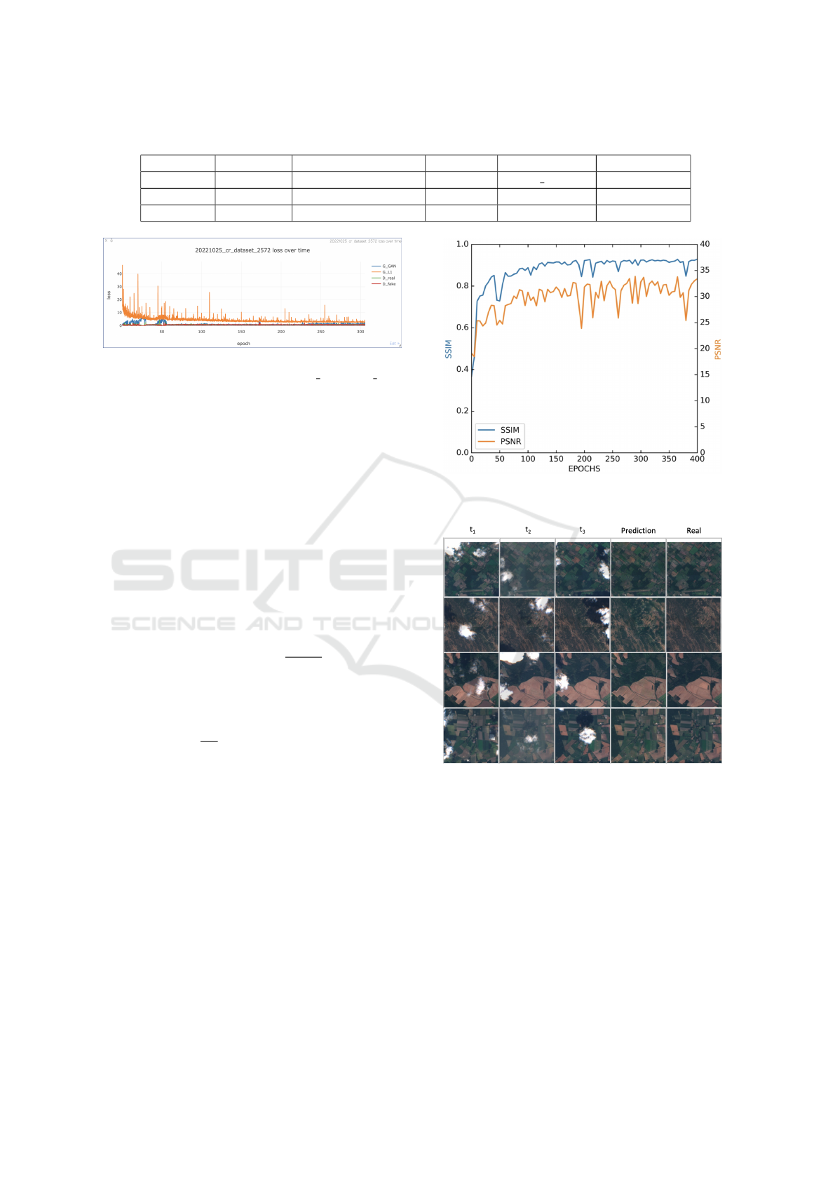
Table 1: Hyperparameter Settings for STGAN Model.

Batch size GAN Loss Initial Learning Rate Iteration Generator Discriminator

20 vanilla 0.0002 400 resnet 9blocks PatchGAN

Beta 1 Lr Policy Load Size Crop Size Pool Size Norm

0.5 linear 286x286 256x256 50 batch

Figure 8: Training loss curves with 300 epochs on our own

datasets, including CGAN, L1 distance, D real and D fake.

3.3 Model Training and Model

Evaluation

We divided the 2572 image pairs into training, vali-

dation, and testing datasets at an 8:1:1 ratio, respec-

tively. Figure 8 illustrates the loss curves observed

during the model’s training process.

The SSIM(Wang et al., 2004) and PSNR metrics,

acquired from the Tensorﬂow library, were used to

evaluate the model. In which PSNR is a widely-used

metric for image quality assessment that gauges the

ﬁdelity of a reconstructed image with respect to the

original cloud-free image. It is deﬁned as follows:

PSNR = 10 · log

(

MAX

MSE

) (4)

Mean-squared error (MSE) is deﬁned as follows:

MSE =

∑

i=1

∑

j=1

[I(i, j)− P(i, j)]

(5)

Where I and P denote real cloud-free images and pre-

dicted images, m, and n are the height and width of

the images, respectively.

To achieve a more precise assessment of the

model’s performance during the training process, we

saved the model weights every ﬁve epochs. Figure 9

showcases the evaluation results on the test dataset,

using the PSNR and SSIM metrics for assessment.

Signiﬁcantly, the model that exhibited the most ex-

ceptional performance attained a SSIM of 0.929 and

a PSNR of 33.4 at epoch 290.

Figure 10 shows the experimental results on

STGAN, including four arbitrarily chosen examples.

The ﬁrst three columns of each example showcase the

temporal cloudy images captured at different times

Figure 9: Evaluation results on test data set with model

weights from 0 to 400 epochs.

Figure 10: Results of learned many-to-one mapping to gen-

erate cloud-free images given a sequence of cloudy images.

(t0, t1, and t2, respectively), while the fourth column

displays the corresponding predicted images. The last

column exhibits the authentic clear images.

4 CONCLUSIONS AND FUTURE

WORK

In this work, we build a new, global, and spatio-

temporal dataset in two versions with image size of

10980x10980 and 256x256. We have randomly se-

lected 2572 images from a total of 57474, and par-

A Global Multi-Temporal Dataset with STGAN Baseline for Cloud and Cloud Shadow Removal

211

titioned them into the train, validation, and test sets

with percentages of 0.8, 0.1, and 0.1 respectively.

The STGAN model shows the state-of-the-art perfor-

mance in our dataset. The PSNR and SSIM reach up

to 33.4 and 0.929 respectively. We hope our dataset

will be widely used, which makes more satellite data

used for further research and applications. We have

made our dataset publicly available at the following

link: https://github.com/zhumorui/SMT-CR.

Our future work will focus on dealing with im-

ages on entire images, as opposed to cropped images.

By processing entire images, we can effectively uti-

lize global spatio-temporal information, while avoid-

ing the risk of errors that may occur at the edges of

cropped images. Furthermore, we will test and com-

pare the different state of art networks on our dataset.

REFERENCES

Cheng, Q., Shen, H., Zhang, L., Yuan, Q., and Zeng, C.

(2014). Cloud removal for remotely sensed images

by similar pixel replacement guided with a spatio-

temporal MRF model. ISPRS Journal of Photogram-

metry and Remote Sensing, 92:54–68. Asked Authors

for Source Code.

Garnot, V. S. F. and Landrieu, L. (2021). Panoptic Segmen-

tation of Satellite Image Time Series with Convolu-

tional Temporal Attention Networks. arXiv.

Gure, M., Ozel, M., Yildirim, H., and Ozdemir, M. (2009).

Use of satellite images for forest ﬁres in area determi-

nation and monitoring. 2009 4th International Con-

ference on Recent Advances in Space Technologies,

pages 27–32.

Helmer, E. and Ruefenacht, B. (2005). Cloud-Free Satellite

Image Mosaics with Regression Trees and Histogram

Matching. Photogrammetric Engineering & Remote

Sensing, 71(9):1079–1089.

Hettiarachchi, P., Nawaratne, R., Alahakoon, D., Silva,

D. D., and Chilamkurti, N. (2021). Rain Streak

Removal for Single Images Using Conditional Gen-

erative Adversarial Networks. Applied Sciences,

11(5):2214.

Isola, P., Zhu, J.-Y., Zhou, T., and Efros, A. A. (2017).

Image-to-image translation with conditional adversar-

ial networks. In Proceedings of the IEEE Conference

on Computer Vision and Pattern Recognition (CVPR).

Kussul, N., Lavreniuk, M., Skakun, S., and Shelestov, A.

(2017). Deep Learning Classiﬁcation of Land Cover

and Crop Types Using Remote Sensing Data. IEEE

Geoscience and Remote Sensing Letters, 14(5):778–

782.

Mao, K., Yuan, Z., Zuo, Z., Xu, T., Shen, X., and Gao,

C. (2019). Changes in Global Cloud Cover Based on

Remote Sensing Data from 2003 to 2012. Chinese

Geographical Science, 29(2):306–315.

Matwin, S., Yu, S., Farooq, F., Albert, A., Kaur, J., and

Gonzalez, M. C. (2017). Using Convolutional Net-

works and Satellite Imagery to Identify Patterns in Ur-

ban Environments at a Large Scale. Proceedings of

the 23rd ACM SIGKDD International Conference on

Knowledge Discovery and Data Mining, pages 1357–

1366.

Ramoino, F., Tutunaru, F., Pera, F., and Arino, O.

(2017). Ten-Meter Sentinel-2A Cloud-Free Compos-

ite—Southern Africa 2016. Remote Sensing, 9(7):652.

Sarukkai, V., Jain, A., Uzkent, B., and Ermon, S. (2019).

Cloud Removal in Satellite Images Using Spatiotem-

poral Generative Networks. arXiv. Source Code:

https://github.com/VSAnimator/stgan.

Sharma, P. K., Jain, P., and Sur, A. (2019). Dual-Domain

Single Image De-Raining Using Conditional Genera-

tive Adversarial Network. 2019 IEEE International

Conference on Image Processing (ICIP), 00:2796–

2800.

Sudmanns, M., Tiede, D., Augustin, H., and Lang, S.

(2020). Assessing global Sentinel-2 coverage dynam-

ics and data availability for operational Earth observa-

tion (EO) applications using the EO-Compass. Inter-

national Journal of Digital Earth, 13(7):768–784.

Szir

anyi, T. and Shadaydeh, M. (2013). Improved segmen-

tation of a series of remote sensing images by using a

fusion mrf model. In 2013 11th International Work-

shop on Content-Based Multimedia Indexing (CBMI),

pages 137–142. IEEE.

Tseng, D.-C., Tseng, H.-T., and Chien, C.-L. (2008). Au-

tomatic cloud removal from multi-temporal SPOT

images. Applied Mathematics and Computation,

205(2):584–600.

Wang, Z., Bovik, A. C., Sheikh, H. R., and Simoncelli, E. P.

(2004). Image Quality Assessment: From Error Vis-

ibility to Structural Similarity. IEEE Transactions on

Image Processing, 13(4):600–612.

Wurm, M., Stark, T., Zhu, X. X., Weigand, M., and

Taubenb

ock, H. (2019). Semantic segmentation of

slums in satellite images using transfer learning on

fully convolutional neural networks. ISPRS Journal

of Photogrammetry and Remote Sensing, 150:59–69.

Zhang, Q., Yuan, Q., Li, J., Li, Z., Shen, H., and Zhang,

L. (2020). Thick cloud and cloud shadow removal

in multitemporal imagery using progressively spatio-

temporal patch group deep learning. ISPRS Journal of

Photogrammetry and Remote Sensing, 162:148–160.

Source Code: https://github.com/qzhang95/PSTCR.

Zhu, J.-Y., Park, T., Isola, P., and Efros, A. A. (2017).

Unpaired image-to-image translation using cycle-

consistent adversarial networks. In Computer Vision

(ICCV), 2017 IEEE International Conference on.

Zhu, Z. and Woodcock, C. E. (2012). Object-based cloud

and cloud shadow detection in Landsat imagery. Re-

mote Sensing of Environment, 118:83–94.

IMPROVE 2023 - 3rd International Conference on Image Processing and Vision Engineering

212