A Study on Hybrid Classical: Quantum Computing Instructions for a

Fragment of the QuickSI Algorithm for Subgraph Isomorphism

Radu-Iulian Gheorghica

∗ a

Faculty of Mathematics and Computer Science, Babes¸-Bolyai University, Cluj-Napoca, Romania

Keywords:

Quantum Computing, Classical Computing, Subgraph Isomorphism.

Abstract:

The purpose of the research presented in this paper is replacing classical computing instructions of a QuickSI

Algorithm (Shang and collaborators, 2008)(Lee and collaborators, 2012) fragment for subgraph isomorphism

with quantum computing instructions that serve the same purpose, but have a much better performance in

terms of execution times. The key results are quantum circuits that can replace speciﬁed instructions in the

QuickSI Algorithm source code. The quantum circuits have the role of oracles which are composed of gates

that manipulate qubits. In the following sections are presented three quantum computing approaches: two for

graph creation and one for generating truly random numbers.

1 INTRODUCTION

In this work it was studied how to obtain the equiv-

alent in quantum computing of several lines of code

from classical computing from a fragment of the

QuickSI algorithm. Also, through this hybrid ap-

proach, this study aims to achieve an easy to under-

stand way of converting classical algorithms into hy-

brid ones. The state of any classical computer can

be represented as a very long set of ones and ze-

roes. Quantum bits can have not only values of one

and zero, but also linear combinations of these values

(IBM Quantum, 2022a). Thus, in principle, a quan-

tum computer can do everything a classical computer

can do. Still, the limitations of quantum computers

consist of the number of qubits available and the min-

imal diversity regarding quantum gates. In time, the

performance of execution times and quantity of data

that can be used will be increased by the availability

of larger numbers of qubits for each quantum com-

puter and the existence of new quantum gates. There-

fore, all classical algorithms can also be performed

on a quantum computer (Lanzagorta and Uhlmann,

2009). Many companies, including Google, Hon-

eywell, IBM, and Intel, have developed gate model

quantum computers. Another approach is known as

quantum annealing, which aims to use the effects

of quantum ﬂuctuations. Instead of formulating the

https://orcid.org/0000-0002-5543-5023

∗

Supervisor Dr. P

arv Bazil, Professor Emeritus

problem in terms of quantum gates, it is expressed

as an optimization problem and the quantum anneal-

ing computer searches for the optimal solution. D-

Wave Systems is a company that offers publicly avail-

able quantum annealing computers (Brown, 2023).

Ullmann’s Algorithm (Ullmann, 1976) pioneered the

search method that was developed for ﬁnding isomor-

phic patterns in 1976. This algorithm the main frame-

work for a signiﬁcant number of newer subgraph iso-

morphism algorithms (Guo, 2022). This study is

made in the context of subgraph isomorphism. In this

problem, we are given two graphs G

and G

, G

be-

ing a smaller graph than G

, and we are asked to test

the existence of a subgraph of G

that is isomorphic

to G

(Erciyes, 2015). The hypothesis investigated is

that any line of code from classical computing can be

converted to quantum computing.

2 EXISTING WORK ON THE

SUBJECT

1. In (Endo and collaborators, 2021) the au-

thors summarise the most basic ideas of hybrid

quantum-classical algorithms and quantum error

mitigation techniques.

2. In (Callison and Chancellor, 2022) the authors

explore very directly the concept of an algo-

rithm being hybrid quantum-classical by build-

ing a deﬁnition based on previous work in ab-

Gheorghica, R.

A Study on Hybrid Classical: Quantum Computing Instructions for a Fragment of the QuickSI Algorithm for Subgraph Isomorphism.

DOI: 10.5220/0011942400003464

In Proceedings of the 18th International Conference on Evaluation of Novel Approaches to Software Engineering (ENASE 2023), pages 505-512

ISBN: 978-989-758-647-7; ISSN: 2184-4895

 2023 by SCITEPRESS – Science and Technology Publications, Lda. Under CC license (CC BY-NC-ND 4.0)

505

straction/representation theory, arguing that what

makes an algorithm hybrid is not directly how it

is run (or how many classical resources it con-

sumes), but whether classical components are cru-

cial to an underlying model of the computation.

3. According to (Callison and Chancellor, 2022),

Shor’s algorithm is far from being a purely quan-

tum algorithm, and should certainly be consid-

ered a hybrid algorithm. The algorithm relies on a

polynomial-time reduction of the factoring prob-

lem to the problem of ﬁnding the order r of a pe-

riodic function. Almost all of the steps are en-

tirely classical The only part of the algorithm that

is quantum is the call to the quantum phase esti-

mation circuit, which forms the core of the order-

ﬁnding subroutine.

3 TERMINOLOGY

1. The qubit - It is the physical carrier of quantum

information (IBM Quantum, 2022b).

2. Quantum circuit - A quantum circuit is a com-

putational routine consisting of coherent quantum

operations on quantum data, such as qubits, and

concurrent real-time classical computation (IBM

Quantum, 2022e)(IBM Quantum, 2022c).

3. Oracle - A function f which returns f (x) = 0 for

all unmarked items x and f (w) = 1 for the win-

ner. To use a quantum computer for this problem,

we must provide the items in superposition to this

function, so we encode the function into a unitary

matrix called an oracle (IBM Quantum, 2022e)

(IBM Quantum, 2022d).

4. Amplitudes - They are complex numbers and each

possible outcome has a corresponding amplitude.

Amplitudes are analogous to conventional prob-

abilities, as the magnitude of the amplitude is

correlated to the chance of measuring that out-

come. Unlike conventional probabilities, ampli-

tudes have phase and can interfere with each other.

According to (IBM Quantum, 2022d) it is the am-

plitude, and not just the probability, that is being

ampliﬁed. In the current case, amplitudes are used

to present a data graph subgraph’s viability of be-

ing the occurence of the query graph (IBM Quan-

tum, 2022c) (IBM Quantum, 2022d).

5. Gates - Classical and quantum operations can be

used to manipulate qubits in a quantum circuit.

Quantum operations include quantum gates, such

as the Hadamard gate, as well as operations that

are not quantum gates, such as the measurement

operation (IBM Quantum, 2022e)(IBM Quantum,

2022f).

6. Hadamard gate - It rotates the states |0⟩ and |1⟩

to |+⟩ and |−⟩, respectively. It is useful for mak-

ing superpositions. If you have a universal gate

set on a classical computer and add the Hadamard

gate, it becomes a universal gate set on a quantum

computer (IBM Quantum, 2022e)(IBM Quantum,

2022a)(IBM Quantum, 2022f).

7. Query graph and data graph - The query graph

is used for searching its occurrences in the data

graph.

8. A classical algorithm, known as a non-quantum

algorithm, is a well-deﬁned sequence of instruc-

tions that is created as a solution to a particular

problem.

9. Hybrid quantum-classical algorithms are regarded

as well-suited for execution on NISQ (noisy

intermediate-scale quantum) devices by combin-

ing quantum computers with classical computers,

and are expected to be the ﬁrst useful applications

for quantum computing (Endo and collaborators,

2021).

10. In the ﬁeld of quantum computing, a quantum al-

gorithm refers to an algorithm that is created to

be executed on a practical quantum computing

model. The most frequently used model for this

goal is the quantum circuit model of computation.

(Nielsen and Chuang, 2000)(Mosca, 2008).

4 THE QuickSI ALGORITHM

FRAGMENT

In this section is presented a fragment of the

QuickSI Algorithm transposed in Python (van

Rossum, 1989) by the author of the current pa-

per.

1: class QuickSIAlgorithm(): {Here is the

creation of two edge lists for the same

graph by using the adjacency matrix of

the graph: 0-based uses the indices

of the matrix as it was created through

numpy (Oliphant and collaborators, 1995).

1-based is the list that will be used by

NetworkX (Hagberg and collaborators, 2005)

to create the graph. The numbers from

this list represent nodes.}

2: edgeList2 0 based = []

3: edgeList2 1 based = []

4: for i in range(0, b.shape[0]) do

5: for j in range(0, b.shape[1]) do

6: if b[i, j] == 1 then

ENASE 2023 - 18th International Conference on Evaluation of Novel Approaches to Software Engineering

506

7: edgeList2 0 based.append([i, j])

8: edgeList2 1 based.append([i + 1, j +

1])

9: end if

10: end for

11: end for{Adding the edges:}

12: graphB.add edges from(edgeList2 1 based)

13: c = np.matrix([[0, 1, 0, 0, 0, 0], [1, 0,

1, 0, 0, 0], [0, 1, 0, 1, 0, 0], [0, 0, 1,

0, 0, 0], [0, 0, 1, 0, 0, 0], [0, 1, 0, 0,

0, 0]])

14: graphC = nx.Graph()

15: graphC.add node(1) c1 = Vertex("N", "c1")

16: graphC.add node(2) c2 = Vertex("C", "c2")

17: graphC.add node(3) c3 = Vertex("C", "c3")

18: graphC.add node(4) c4 = Vertex("C", "c4")

19: graphC.add node(5) c5 = Vertex("C", "c5")

20: graphC.add node(6) c6 = Vertex("O", "c6")

21: edgeList3 1 based = []

22: for i in range(0, c.shape[0]) do

23: for j in range(0, c.shape[1]) do

24: if c[i,j] == 1 then

25: edgeList3 1 based.append([i+1,j+1])

26: end if

27: end for

28: end for{In the following part is

attempted the implementation of a QI

Sequence (Lee and collaborators, 2012)

for a graph. } {A data graph from (Lee

and collaborators, 2012):}

{Nodes:}

29: a1 = Vertex("N", "a1"), a2 = Vertex("C",

"a2"),

a3 = Vertex("C", "a3"), a4 = Vertex("C",

"a4"),

a5 = Vertex("C", "a5"), a6 = Vertex("C",

"a6"),

30: graphA node list = [a1, a2, a3, a4, a5,

a6] {Adjacency matrix for an undirected

graph having edge weights:}

31: a = np.matrix([[0, 1.40, 0, 0, 0, 0], [1,

0, 45.10, 0, 0, 5.10], [0, 1, 0, 5.10, 0,

0], [0, 0, 1, 0, 5.10, 0], [0, 0, 0, 1, 0,

5.10], [0, 1, 0, 0, 1, 0]])

32: graphA = nx.Graph()

33: graphA.add node(a1), graphA.add node(a2),

graphA.add node(a3), graphA.add node(a4),

graphA.add node(a5), graphA.add node(a6)

34: edgeList = [(a1, a2), (a2, a1), (a2, a3),

(a2, a6), (a3, a2), (a3, a4), (a4, a3),

(a4, a5), (a5, a4), (a5, a6), (a6, a2),

(a6, a5)]

{Iterating the adjacency matrix:}

35: for i in range(0, a.shape[0]) do

36: for j in range(0, a.shape[1]) do

37: if a[i, j] != 0 and i < j then {i

< j will select the elements above

the main diagonal of the adjacency

matrix}

38: graphA.add

edge(graphA node list[i],

graphA node list[j], weight=a[i,j])

39: end if

40: end for

41: end for

42: P = graphA.edges(data=True)

43: qw = graphA

44: P 2 = []

45: if len(P) > 1 then

46: for i in range(0, len(P)-1) do

47: if qw.degree(P[i][0])

+ qw.degree(P[i][1]) ≤

qw.degree(P[i+1][0]) +

qw.degree(P[i+1][1]) then

48: P 2.append(P[i]) {P[i] is "e"}

49: end if

50: end for

51: i = random.randrange(0, len(P 2))

52: selectedEdgeFromP 2 = P 2[i]

53: end if

In order for a quantum computer to work with the in-

put data, a methodology is needed in order encode it

for the oracle. Thus, an index will have to be assigned

to the query data. For example, a query graph can

have an index 00. Then the oracle will look for this

index by using gates in a quantum circuit that amplify

the amplitude for the outcome 00 (Bick, 2018)(Mc-

Caig, 2021).

The part of the code at lines 1 - 12 represents the cre-

ation of the ﬁrst graph for the algorithm. The second

graph is created between the lines 13 and 28. The

third graph is created between lines 29 and 41. Let’s

consider that each of these graphs has 6 nodes. Lines

of code from classical computing will be transformed

into quantum computing. The quantum computing

equivalent for this, according to the terminology, is

the following. There are two approaches.

1. There are three input graphs, thus there were cre-

ated three quantum circuits, each graph being en-

coded in a circuit.

2. Let’s consider, for example, three quantum cir-

cuits, each having 6 qubits. Just like it was men-

tioned at the ﬁrst point, a circuit belongs to a

graph. In this case, each graph is divided in parts

which are assigned to different outcomes. The

qubits interact between each other and exchange

information. From here results that the aforemen-

tioned hypothesis is valid because the nodes of the

graph also interact with each other.

For larger numbers of qubits exist larger numbers of

outcomes. For 6 qubits there are 2

= 64 outcomes,

for 15 qubits there are 2

= 32768 outcomes and

A Study on Hybrid Classical: Quantum Computing Instructions for a Fragment of the QuickSI Algorithm for Subgraph Isomorphism

507

for 300 qubits there are 2

300

= 2.037036e + 90 out-

comes. Consequently, larger graphs can be stored

when the quantum computer has a larger number of

qubits. From this can be considered that the max-

imum capacity of a quantum computer’s number of

qubits represents a graph in itself as seen in Figures 1

and 2. In those ﬁgures, the nodes represent the qubits

and the edges are the connections between them. The

colors of the nodes represent the value readout assign-

ment error. The colors of the connections represent

the value of the CNOT error (IBM Quantum, 2022g)

(IBM Quantum, 2022h).

Figure 1: The undirected graph of the qubits for the

ibm nairobi quantum computer (IBM Quantum, 2022g).

Figure 2: The undirected graph of the qubits for the

ibm oslo quantum computer (IBM Quantum, 2022h).

In time, after the quantum internet will be more

evolved, quantum computers will be able to transfer

data between each other. The basis for this is quan-

tum entanglement. According to the deﬁnition of the

amplitudes speciﬁed in the terminology at section 3,

they interfere with each other. In conclusion, we can

consider that interference and quantum entanglement

can be the equivalent of the interactions between the

nodes of the encoded graph. The performance eval-

uation of the quantum circuits is based on extremely

small execution times. In Tables 1, 2 and 5 are pre-

sented the execution times of quantum circuits repre-

sented in Figures 3, 5, 7, 9, 11, 13, 15 and 17. Each

circuit was executed 8192 times by quantum comput-

ers. For exempliﬁcation of the execution speed, each

table also contains the run time of just one execution

for each quantum circuit.

5 THE FIRST APPROACH

In the following section is presented a procedure for

graph creation using quantum computing after which

there have been presented test cases, results and dis-

cussion. We can encode each graph in a separate out-

come. For example, the ﬁrst input graph can be en-

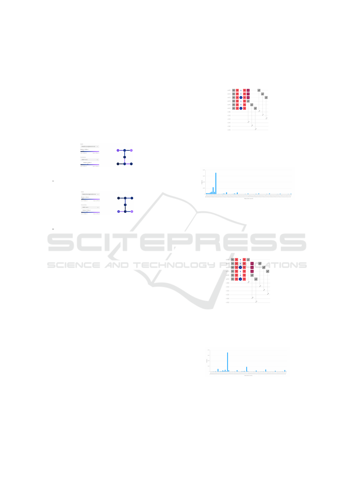
coded in the outcome 000111. For this, in Figure 3 is

presented the quantum circuit associated with this op-

eration. In Figure 3 were used the reset operation,

the Hadamard, Toffoli and Y gates, ﬁnishing with

the measurement operation. The Toffoli gates create

quantum entanglement between qubits.

Figure 3: The quantum circuit associated with the ﬁrst input

graph.

In Figure 4 the ampliﬁed amplitude for the 000111

outcome represents the ﬁrst graph.

Figure 4: The histogram with the ampliﬁed amplitudes for

the circuit presented in Figure 3.

The second graph has been encoded in the out-

come 001110. The corresponding circuit is presented

in Figure 5. For the test in this circuit were used the

reset operation, the Hadamard, Toffoli and Y gates,

ﬁnalizing with the measurement operation.

Figure 5: The quantum circuit associated with the second

input graph.

In the histogram from Figure 6, the ampliﬁed am-

plitude for the outcome 001110 represents the second

graph.

Figure 6: The histogram with the ampliﬁed amplitudes for

the circuit presented in Figure 5.

The third graph is encoded in the outcome

011100. For this graph, the circuit is presented in

Figure 7. This circuit also uses the reset operation,

the Hadamard, Toffoli and the Y gates, ﬁnishing with

the measurement operation.

ENASE 2023 - 18th International Conference on Evaluation of Novel Approaches to Software Engineering

508

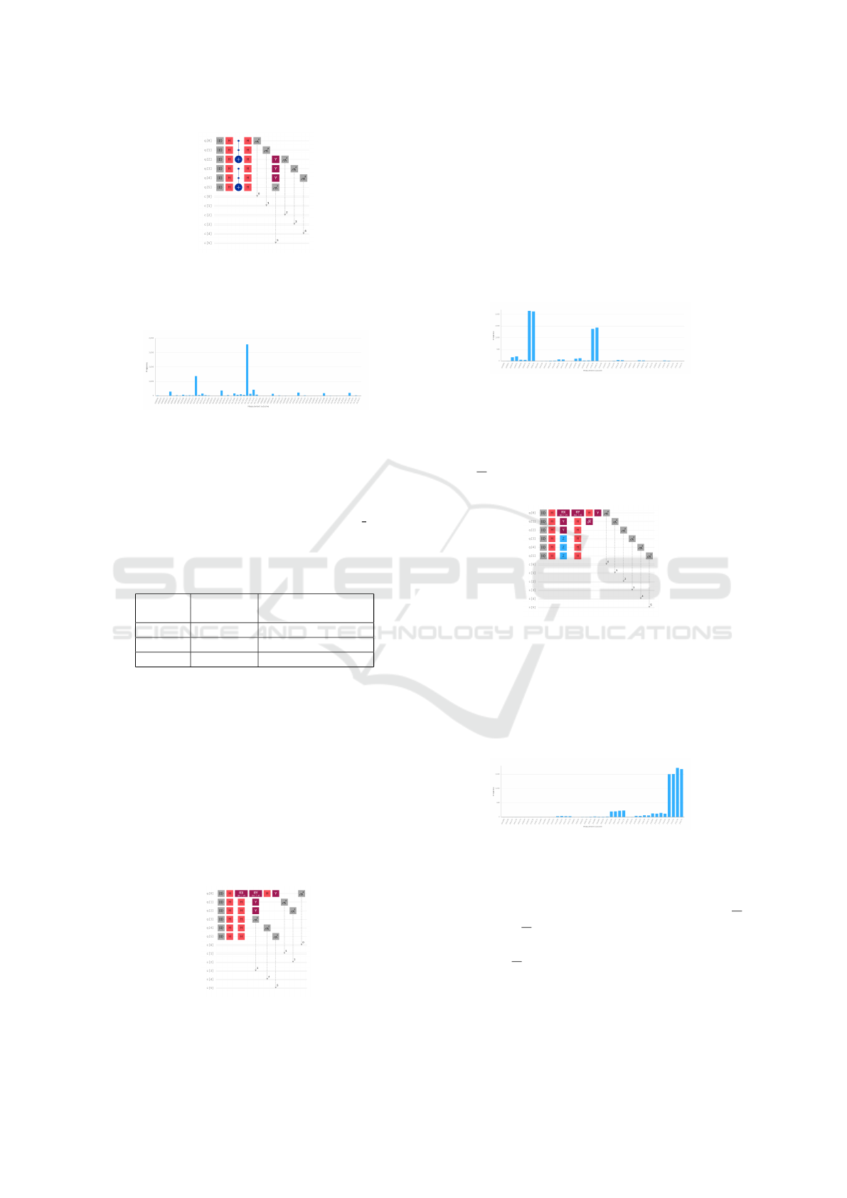
Figure 7: The quantum circuit associated with the third in-

put graph.

In Figure 8 the ampliﬁed amplitude for 011100

represents the third graph.

Figure 8: The histogram with the ampliﬁed amplitudes for

the circuit presented in Figure 7.

The other less ampliﬁed amplitudes from Figures

4, 6 and 8 are considered other graphs that have differ-

ent encodings. The circuits in Figures 3, 5 and 7 were

executed on the real quantum computer ibm nairobi

(IBM Quantum, 2022g) having 7 qubits.

Table 1: Execution times for the circuits in Figures 3, 5 and

7. Each circuit was executed 8192 times.

Circuit Execution Execution times

times (sec) for a single run (sec)

Figure 3 6.8 0.00083

Figure 5 6.6 0.0008

Figure 7 6.9 0.00084

6 THE SECOND APPROACH

In this section is presented a second procedure for

graph creation using quantum computing. Afterwards

there have been presented test cases, results and dis-

cussion. Let’s consider each of the 6 nodes of the ﬁrst

input graph be associated with different outcomes.

The corresponding circuit is presented in Figure 9. It

uses the reset operation, the Hadamard, RX, RY and

Y gates. After these gates the measurement operation

has been used.

Figure 9: The quantum circuit associated with the ﬁrst input

graph.

There are two amplitudes that are ampliﬁed more than

the rest as seen in Figure 10: 000110 and 000111.

The graph is divided in half: three nodes for the ﬁrst

ampliﬁed amplitude and the other three nodes for the

second ampliﬁed amplitude. Also in Figure 10 can be

seen similar encodings of the graph, but for less am-

pliﬁed amplitudes. For example, 010110 and 010111.

Each node is a smaller part of the larger graph. Each

part of a graph, according to how the user wants to

encode it, can be associated to an outcome.

Figure 10: The histogram with the ampliﬁed amplitudes for

the circuit presented in Figure 9.

The quantum circuit from Figure 11 is associated

with the second input graph. This circuit is created

with the reset operation, the Hadamard, RX, RY, Y, Z

and

√

X gates, ending with the measurement opera-

tion.

Figure 11: The quantum circuit associated with the second

input graph.

In Figure 12 the second input graph is divided in

four parts: two nodes for 111100, another two nodes

for 111101, one node for 111110 and one node for

111111. Also in Figure 12 are presented similar en-

codings of the graph. For example: 101100, 101101,

101110 and 101111.

Figure 12: The histogram with the ampliﬁed amplitudes for

the circuit presented in Figure 11.

The quantum circuit presented in Figure 13 cor-

responds to the third input graph. This circuit uses

the reset operation, the Hadamard, RX, RY and

√

gates. Each

√

X gate used has a control qubit associ-

ated to it. If a control qubit has the state |1⟩, then its

belonging

√

X gate will be executed. Afterwards, the

measurement operation has been used.

A Study on Hybrid Classical: Quantum Computing Instructions for a Fragment of the QuickSI Algorithm for Subgraph Isomorphism

509

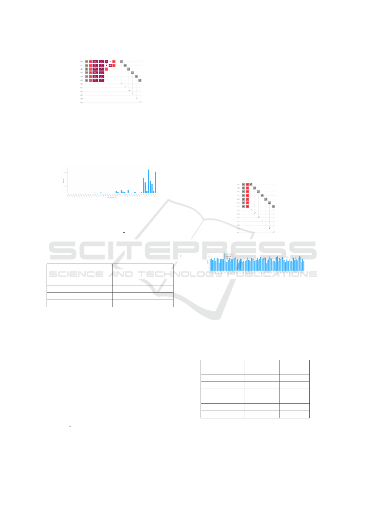
Figure 13: The quantum circuit associated with the third

input graph.

In Figure 14 the third input graph is divided in

three parts: two nodes for 111000, two nodes for

111011 and the last two nodes for 111111. In the

same ﬁgure are represented similar encodings of this

graph: 111001, 111100 and 111101.

Figure 14: The histogram with the ampliﬁed amplitudes for

the circuit presented in Figure 13.

The circuits in Figures 9, 11 and 13 were executed on

the real quantum computer ibm oslo (IBM Quantum,

2022h) having 7 qubits.

Table 2: Execution times for the circuits in Figures 9, 11

and 13. Each circuit was executed 8192 times.

Circuit Execution Execution times

times (sec) for a single run (sec)

Figure 9 6.4 0.00078

Figure 11 6.3 0.00076

Figure 13 6.6 0.0008

7 TRULY RANDOM NUMBERS

At line of code number 51 from the fragment of the

QuickSI Algorithm in section number 4 is presented

the pseudorandom generation of a value from a given

range of values. In quantum computing truly random

values can be generated according to (Li and collab-

orators, 2021)(Q-munity, 2022). Through the use of

the Hadamard gate and thus, the superposition of all

the possible numbers that can be generated, true ran-

domness can be achieved. The author of (Q-munity,

2022) has used a quantum simulator to obtain the

probabilities of occurrence for each value from 0 to

7. For the tests in this paper, the real quantum com-

puter ibm oslo (IBM Quantum, 2022h) has been used

having 7 qubits. In Figure 15 is presented the circuit

for this and in Figure 16 are all the possible numbers

that can be generated with 7 qubits. This amounts to

a total of 2

= 128 possible numbers. This means that

the qubits will be in a superposition of all of these

numbers and in the following histograms we can see

the probabilities of each of those numbers to occur. In

order to highlight the randomness for the occurence of

the numbers, the circuits from Figures 15 and 17 were

executed, resulting two different histograms. The cir-

cuits in Figures 15 and 17 use the reset operation,

the Hadamard gate and the measurement operation.

The two histograms show different sets of occurrence

probabilities for the 128 numbers. For example, num-

ber 0 is encoded in the 0000000 outcome, number 1

is encoded in the 0000001 outcome, number 2 is en-

coded in the 0000010 outcome and so on until the last

number which is 127 that is encoded in 1111111. This

applies for the histograms in Figures 16 and 18.

Figure 15: The circuit for the ﬁrst random number.

Figure 16: Histogram for the circuit from Figure 15. Here

are the most frequent numbers from the 128 positions men-

tioned.

Table 3 belongs to the histogram in Figure 16. The

measurement outcomes are the computational basis

states, the frequencies are the ampliﬁed amplitudes

for those outcomes and the encoded numbers are as-

sociated to the speciﬁed outcomes. The number with

the highest probability to occur is number 19.

Table 3: Histogram from Figure 16 in detailed form.

Measurement Frequency Encoded

outcome number

”0000000” ”64” 0

”0000001” ”66” 1

. . . . . . . . .

”0010011” ”99” 19

. . . . . . . . .

”1111111” ”53” 127

ENASE 2023 - 18th International Conference on Evaluation of Novel Approaches to Software Engineering

510

Figure 17: The circuit for the second random number.

Figure 18: Histogram for the circuit from Figure 17. Here

are the most frequent numbers from the 128 positions men-

tioned.

Table 4 is associated with the histogram presented

in Figure 18. The measurement outcomes represent

computational basis states, the frequencies are the

ampliﬁed amplitudes for those outcomes and the en-

coded numbers are associated to the speciﬁed out-

comes. The number with the highest probability to

occur is number 91.

Table 4: Histogram from Figure 18 in detailed form.

Measurement Frequency Encoded

outcome number

”0000000” ”54” 0

”0000001” ”67” 1

. . . . . . . . .

”1011011” ”86” 91

. . . . . . . . .

”1111111” ”66” 127

The circuits in Figures 15 and 17 were executed on

the real quantum computer ibm oslo (IBM Quantum,

2022h) having 7 qubits.

Table 5: Execution times for the circuits in Figures 15 and

17. Each circuit was executed 8192 times.

Circuit Execution Execution times

times (sec) for a single run (sec)

Figure 15 6.4 0.00078

Figure 17 6.3 0.00076

8 ALTERNATIVE APPROACHES

An alternative approach to evaluating the execution is

the Qiskit library (MD A. SAJID et al., 2021). In-

stead of using the Circuit Composer (IBM Quantum,

2022e), it offers much more control through the use

of the Python programming language to formulate

quantum circuits and send them for execution to the

quantum computers directly from the code. As more

parts of the classical algorithm are converted into their

quantum counterparts, the less will matter the clas-

sical hardware platform that is used. The author of

this paper considers that with the right combination

of quantum gates, an algorithmic conversion is possi-

ble with a minimal time of work.

9 CONCLUSIONS

In this paper were presented three quantum comput-

ing approaches for replacing classical computing in-

structions in a fragment of the QuickSI Algorithm for

subgraph isomorphism. In the ﬁrst and the second ap-

proaches, the quantum circuits created are the equiv-

alent for creating graphs for the algorithm. The third

quantum computing approach presented has the role

of generating truly random numbers. Starting from

the premise that for example, a classical computer can

exist in only one state out of 25, while a quantum

computer can exist in all 25 states at the same time

due to superposition, through the superiority of this

omnipresence and quantum entanglement of quantum

bits, the next step is the improvement, perfecting of

existing quantum gates and developing new ones.

ACKNOWLEDGEMENTS

I acknowledge the use of IBM Quantum services for

this work. The views expressed belong to the author,

and do not reﬂect the ofﬁcial policy or position of

IBM or the IBM Quantum team.

REFERENCES

Bick (2018). https://quantumcomputing.stackexchange.com

/questions/2149/grovers-algorithm-what-to-input-to-

oracle.

Brown, R. (2023). https://www.quantumcomputinginc.com

/blog/quantum-annealing-gate/.

Callison, A. and Chancellor, N. (2022). Hy-

brid quantum-classical algorithms in the noisy

intermediate-scale quantum era and beyond . DOI:

https://doi.org/10.1103/PhysRevA.106.010101.

Endo, S. and collaborators (2021). Hybrid Quantum-

Classical Algorithms and Quantum Error Mitigation.

Journal of the Physical Society of Japan, 90, 032001

(2021) 10.7566/JPSJ.90.032001.

A Study on Hybrid Classical: Quantum Computing Instructions for a Fragment of the QuickSI Algorithm for Subgraph Isomorphism

511

Erciyes, K. (2015). COMPLEX NETWORKS An Algo-

rithmic Perspective. ISBN-13: 978-1-4665-7167-9

(eBook - PDF), CRC Press Taylor & Francis Group.

Guo, M. (2022). A (Sub)graph Isomorphism Identiﬁcation

Theorem. PhD thesis, Swinburne University of Tech-

nology, Melbourne, Australia.

Hagberg, A. and collaborators (2005).

https://networkx.org/.

IBM Quantum (2022a). https://quantum-

computing.ibm.com/composer/docs/iqx/guide/creating-

superpositions.

IBM Quantum (2022b). https://quantum-

computing.ibm.com/composer/docs/iqx/guide/the-

qubit.

IBM Quantum (2022c). https://quantum-

computing.ibm.com/composer/docs/iqx/terms-

glossary/.

IBM Quantum (2022d). https://quantum-

computing.ibm.com/composer/docs/iqx/guide/grovers-

algorithm.

IBM Quantum (2022e). IBM Quantum Expe-

rience Circuit Composer. https://quantum-

computing.ibm.com/composer/ﬁles/new.

IBM Quantum (2022f). IBM Quantum Experi-

ence Operations Glossary. https://quantum-

computing.ibm.com/lab/docs/iql/operations glossary/.

IBM Quantum (2022g). ibm nairobi v1.2.0, 7 qubits,

processor type: Falcon r5.11H . https://quantum-

computing.ibm.com.

IBM Quantum (2022h). ibm oslo v1.0.14, 7 qubits,

processor type: Falcon r5.11H . https://quantum-

computing.ibm.com.

Lanzagorta, M. and Uhlmann, J. K. (1 January 2009).

Quantum Computer Science. Morgan & Claypool

Publishers. ISBN 9781598297324.

Lee, J. and collaborators (2012). An in-depth comparison of

subgraph isomorphism algorithms in graph databases.

PVLDB.

Li, Y. and collaborators (2021). Quantum random

number generator using a cloud supercon-

ducting quantum computer based on source-

independent protocol. Sci Rep 11, 23873 (2021).

https://doi.org/10.1038/s41598-021-03286-9.

McCaig, X. (2021). https://quantumcomputing.

stackexchange.com/questions/16350/how-can-

grovers-algorithm-be-implemented-when-having-a-

string-or-other-data-typ.

MD A. SAJID et al. (2021). Qiskit: An Open-source Frame-

work for Quantum Computing. DOI: 10.5281/zen-

odo.2573505.

Mosca, M. (2008). Quantum algorithms.

https://arxiv.org/abs/0808.0369.

Nielsen, M. A. and Chuang, I. L. (2000). Quantum Compu-

tation and Quantum Information. Cambridge Univer-

sity Press. ISBN 978-0-521-63503-5.

Oliphant, T. and collaborators (1995). The fundamen-

tal package for scientiﬁc computing with Python.

https://numpy.org.

Q-munity (2022). https://www.qmunity.tech/tutorials/quantum-

random-number-generator.

Shang, H. and collaborators (2008). Taming Veriﬁca-

tion Hardness: An Efﬁcient Algorithm for Test-

ing Subgraph Isomorphism. Proc. VLDB Endow.,

1(1):364–375.

Ullmann, J. R. (1976). An algorithm for subgraph isomor-

phism. J. ACM, 23(1):31–42.

van Rossum, G. (1989). Python Software Foundation.

https://www.python.org/.

ENASE 2023 - 18th International Conference on Evaluation of Novel Approaches to Software Engineering

512