Beyond the Third Dimension: How Multidimensional Projections and

Machine Learning Can Help Each Other

Alexandru Telea

Department of Information and Computing Science, Utrecht University, Netherlands

Keywords:

Multidimensional Projections, Visual Quality Metrics, Explainable AI.

Abstract:

Dimensionality reduction (DR) methods, also called projections, are one of the techniques of choice for visu-

ally exploring large high-dimensional datasets. In parallel, machine learning (ML) and in particular deep learn-

ing applications are one of the most prominent generators of large, high-dimensional, and complex datasets

which need visual exploration. As such, it is not surprising that DR methods have been often used to open the

black box of ML methods. In this paper, we explore the synergy between developing better DR methods and

using them to understand and engineer better ML models. Speciﬁc topics covered address selecting suitable

DR methods from the wide arena of such available techniques; using ML to create better, faster, and simpler

to use direct and inverse projections; extending the projection metaphor to create dense representations of

classiﬁers; and using projections not only to explain, but also to improve, ML models. We end by proposing

several high-impact directions for future work that exploit the outlined ML-DR synergy.

1 INTRODUCTION

Machine learning (ML) techniques support tasks such

as classiﬁcation and regression and have become fun-

damental instruments in daily practice in a myriad of

ﬁelds. Developments in the past decade have made

such techniques increasingly accurate, computation-

ally scalable, but most importantly, able to address

efﬁciently and effectively an increasing range of prob-

lems such as image analysis (e.g., classiﬁcation, seg-

mentation, and restoration), sentiment identiﬁcation,

natural language processing, to mention just a few.

The advent of deep learning (DL) techniques coupled

with recent advances in GPU and parallel computing

has massively simpliﬁed the ease of creating trained

ML models to solve these problems at industrial scale.

Dimensionality reduction (DR), also called pro-

jection, is a popular technique for visualizing high-

dimensional datasets by low-dimensional scatterplots.

Globally put, a good projection scatterplot captures

well the so-called data structure present in the orig-

inal high-dimensional data in terms of point clus-

ters, outliers, and correlations (Nonato and Aupetit,

2018; Espadoto et al., 2019a; Lespinats and Aupetit,

2011). As such, high-quality projections allow users

to reason about the data structure by exploring the vi-

sual structure of the low-dimensional scatterplots they

produce. Tens of different DR techniques (Espadoto

https://orcid.org/0000-0003-0750-0502

et al., 2019a) have been designed to address the sev-

eral requirements one has for this class of methods,

such as computational scalability, ease of use, stabil-

ity vs noise or small data changes, projecting addi-

tional points along those existing in an original dataset

(out-of-sample ability), and visual quality that pre-

serves the high-dimensional data structure.

ML and DR techniques, while having emerged

from different ﬁelds, share a key similarity: They

both deal with high-dimensional data – a challeng-

ing endeavor. In ML, such data are the so-called

features used during training and inference by mod-

els. In DR, such data represent the samples, or obser-

vations, whose data structure we aim to understand

by means of low-dimensional scatterplots. The two

ﬁelds also share other important commonalities: ML

strongly needs methods to open up the ‘black box’

formed by architecting, training, and using the mod-

els it creates, and many such models are visual, like

the DR scatterplots. Conversely, the task of creating

high-quality projections from high-dimensional data,

with guaranteed stability, out-of-sample ability, gen-

eralizability, and computational scalability shares all

typical requirements met by ML engineering.

In this paper (and related talk), we aim to pro-

vide an overview of the research at the crossroads

of ML and DR with a particular emphasis on high-

lighting commonalities between the two ﬁelds and re-

cent ways in which they can beneﬁt from each oth-

Telea, A.

Beyond the Third Dimension: How Multidimensional Projections and Machine Learning Can Help Each Other.

DOI: 10.5220/0011926400003417

In Proceedings of the 18th International Joint Conference on Computer Vision, Imaging and Computer Graphics Theory and Applications (VISIGRAPP 2023) - Volume 5: VISAPP, pages

5-16

ISBN: 978-989-758-634-7; ISSN: 2184-4321

 2023 by SCITEPRESS – Science and Technology Publications, Lda. Under CC license (CC BY-NC-ND 4.0)

ers’ advances. We start by a short overview of ML

and DR that outlines common aspects of these two

ﬁelds (Sec. 2). We next outline how DR methods are

used to assist ML engineering tasks (Sec. 3). Next, we

discuss how the converse fertilization occurs, namely

ML methods being used to create better DR tech-

niques (Sec. 4). Section 5 merges the insights of

the previous two sections and outlines high-potential

future research directions in which the DR and ML

ﬁelds can beneﬁt from each other. Finally, Section 6

concludes the paper.

2 BACKGROUND

Providing a full introduction of both ML and DR is

out of scope of thos paper. This section aims to pro-

vide a brief outline of the key concepts in the two

ﬁelds which are needed to follow the further discus-

sion and, importantly, highlight commonalities of ML

with DR that next lead to cross-fertilization.

2.1 Machine Learning

We start by listing some notations. Let D = {x

}

be a dataset of N-dimensional samples or points x

1 ≤ i ≤ N. A point x

= (x

, . . . , x

) consist of n

components x

, also called feature or attribute values.

Without generality loss, we assume next for simplic-

ity that each of these is a real-value, i.e., x

∈ R

. The

sets X

= (x

, . . . , x

), 1 ≤ i ≤ N are called the fea-

tures, or dimensions, of the entire dataset D. Sim-

ply put, D can be seen as a table having N rows (one

per sample) and n columns (one per dimension). An

annotated dataset D

associates an additional value

∈ A to each sample x

of a given dataset D.

Machine learning aims to create so-called mod-

els f : R

→ A which, when applied to a so-called

test set D

⊂ D

, deliver the expected annotations,

i.e., d( f (x

), y

) ≃ 0, for ideally all x

∈ D

. Here,

d : A × A → R

is a distance function used to com-

pare the so-called ground-truth annotations y

with the

model’s predictions f (x

), e.g., an L

norm. Models

f are built by using a so-called training set D

⊂ D

∩D

= ∅, to adjust f ’s parameters so as to achieve

the above-mentioned goal. Two main types of models

exist in ML. Classiﬁers use an annotation set having

categorical values (also called labels), in which case

one strives for d = 0. Regressors use an annotation

set having real values (in one or more dimensions), in

which case one strives for d ≃ 0.

Many methods exist to measure the performance

of ML models. The most widespread such methods

measure several so-called quality metrics on the train-

ing set (training performance) and, separately, on the

unseen test set (testing performance). Common met-

rics include accuracy, precision, recall, F-score, and

Cohen’s kappa score. More advanced methods take

into account hyperparameters that allow optimizing

between precision and recall, e.g. the Receiver Oper-

ator Characteristic (ROC) curve and area underneath.

Recent surveys of such metrics and related bench-

marks are given in (Botchkarev, 2019; Jiang et al.,

2020; Thiyagalingam et al., 2022).

2.2 Dimensionality Reduction

Consider a high-dimensional dataset D deﬁned as for

the ML context (Sec. 2.1). A dimensionality reduc-

tion technique, or projection P, is a function that maps

D to P(D) = {y

}, where y

∈ R

is the projection of

. Typically q ≪ n, yielding 2D projections (q = 2)

and 3D projections (q = 3) that are used to visual-

ize D by depicting the respective scatterplots. Pro-

jections aim to preserve the so-called structure of the

dataset D. Intuitively put, this means that patterns in

D such as clusters of densely packed points, outliers,

and gaps between such point formations, should be

visible in P(D).

How well a projection preserves data structure is

measured by several quality metrics. A quality metric

is a function M(D, P(D)) → R

that tells how well

the scatterplot P(D) captures aspects of the dataset D.

Such metrics can be roughly divided into those that

measure distance preservation between R

and R

such as normalized stress and the Shepard diagram

correlation; and metrics that look at how well (small)

neighborhoods of points are preserved between D and

P(D), such as trustworthiness, continuity, or, more

speciﬁc ones, e.g. Kullback-Leibler divergence. Ex-

tensive surveys of projection quality metrics are given

in (Nonato and Aupetit, 2018; Espadoto et al., 2019a).

2.3 Common Sspects of ML and DR

Tens, if not hundreds, of algorithms and techniques

have been proposed for both ML and DR. As our goal

is to highlight ways in which ML can help DR (and

conversely), we next do not discuss such speciﬁc al-

gorithms in detail. Rather, we focus our analysis on

common aspects of the two ﬁelds. To this end, it is

already important to note that both ML models f and

DR projection methods P can be seen as specialized

cases of inference. More speciﬁcally, P can be seen

as a particular type of regressor from R

to R

. Given

this, we next use the notation X to jointly denote an

ML model or DR algorithm, when distinguishing be-

VISIGRAPP 2023 - 18th International Joint Conference on Computer Vision, Imaging and Computer Graphics Theory and Applications

tween the two is not important.

Without claiming full coverage, we identify the

following key aspects that both ML and DR tech-

niques X strive to achieve:

Genericity. X should be readily applicable to any

dataset D – that is, of any dimensionality, attribute

types, and provenance application domain.

Accuracy. X should deliver highly accurate results

(inferences for ML; projection scatterplots for DR) as

gauged by speciﬁc quality metrics in the two ﬁelds.

Scalability. X should scale well computationally with

the number of samples N and dimensions n – ideally,

X should be linear in both N and n. In practice, X

should be readily able to handle datasets with millions

of samples and hundreds of dimensions on commod-

ity hardware at interactive rates. This further on en-

ables the use of X in visual analytics scenarios where

the iterative and interactive exploration of complex

hypotheses via data visualization is essential.

Out of Sample (OOS). An operator X is said to be

OOS if it can extrapolate its behavior beyond the data

from which it was constructed. In ML, this usually

means that the model f extrapolates from a training

set D

to an unseen test set D

and beyond. By anal-

ogy, a projection P is OOS if, when extending some

dataset D with additional samples D

′

, the projection

P(D ∪ D

′

) ideally keeps the points originally in D

at the locations they had in P(D), i.e., P(D ∪ D

′

) =

P(D) ∪ P(D

′

). This is essential in scenarios where

one has a growing dataset to be projected. Existing

points should not change their existing projection lo-

cations if we want to help users maintain their mental

map when interpreting the projection. As most ML

methods are OOS by design, they can be potentially

used to design OOS projections (Sec. 4).

Stability. Small changes in the input dataset D should

only lead to small changes in the output dataset X(D).

If not, then noise-level perturbations in D will mas-

sively affect the resulting inference X(D) thereby ren-

dering such results potentially unusable and/or mis-

leading. Note that stability is related but not the same

as OOS: An OOS algorithm needs to be stable by def-

inition but not all stable algorithms have OOS abil-

ity (Vernier et al., 2021; Espadoto et al., 2019a). Sim-

ilarly, large-scale changes in D should arguably lead

to correspondingly large changes in X(D). We discuss

this aspect in more detail when outlining the chal-

lenges of dynamic projections (Sec. 5.2).

Availability. X should be readily available to prac-

titioners in terms of documented open-source code.

While sometimes neglected, this is a key requirement

for ML and DR algorithms to become impactful in

practice.

Most ML techniques in existence comply by de-

sign with the above properties. However, not all DR

techniques do the same. As we shall see in Sec. 4,

ML can be used to construct DR techniques, thereby

making the latter techniques inherit all the desirable

properties of the former.

3 DR FOR ASSISTING ML

Given the close relation between DR and ML outlined

above, it is not surprising that DR has been used as a

visual analysis tool to assist model engineering. We

next discuss several prominent cases of such usage of

DR.

3.1 Assessing and Improving Classiﬁers

Arguably the most frequent use of DR for ML engi-

neering is to create a projection of a training or test

set, with points colored by class and/or correct-vs-

wrong classiﬁcation, and use it to assess the model’s

working. Indeed, since (a) a projection places sim-

ilar samples close to each other and (b) a classi-

ﬁer labels similar samples similarly, then the visual

structure of the projection should convey insights on

how easily separable are samples of different classes.

While this intuition has been long used, it is only re-

cently that a formal study of this correlation was pre-

sented (Rauber et al., 2017b). In the respective work,

the authors show that a dataset D which creates a pro-

jection P(D) in which classes are well separated (as

measured e.g. by the neighborhood hit metric) will be

far easier classiﬁable than a dataset whose projection

shows intermixed points of different labels. The pro-

jection P(D) thus becomes a ‘proxy’ for the ease of

classifying D regardless of the type of classiﬁer be-

ing used. This helps one in assessing classiﬁcation

difﬁculty before actually embarking in the expensive

cycle of classiﬁer design-train-test.

Figure 1 illustrates the above. Images (a) and

(b) show the two-class Madelon dataset (Guyon et al.,

2004) (n = 500 features) classiﬁer by KNN and Ran-

dom Forests (RFC) respectively, with samples pro-

jected by t-SNE (van der Maaten and Hinton, 2008)

and colored by class. The two projections show a

very poor separation of the two classes, in line with

the obtained accuracies AC = 54% and AC = 66%.

Images (c) and (d) show the same dataset where ex-

tremely randomized trees (Geurts et al., 2006) was

used to select n = 20 features. The projections show

a much higher visual separation of the two classes,

in line with the obtained accuracies AC = 88% and

AC = 89%. Numerous other examples in (Rauber

Beyond the Third Dimension: How Multidimensional Projections and Machine Learning Can Help Each Other

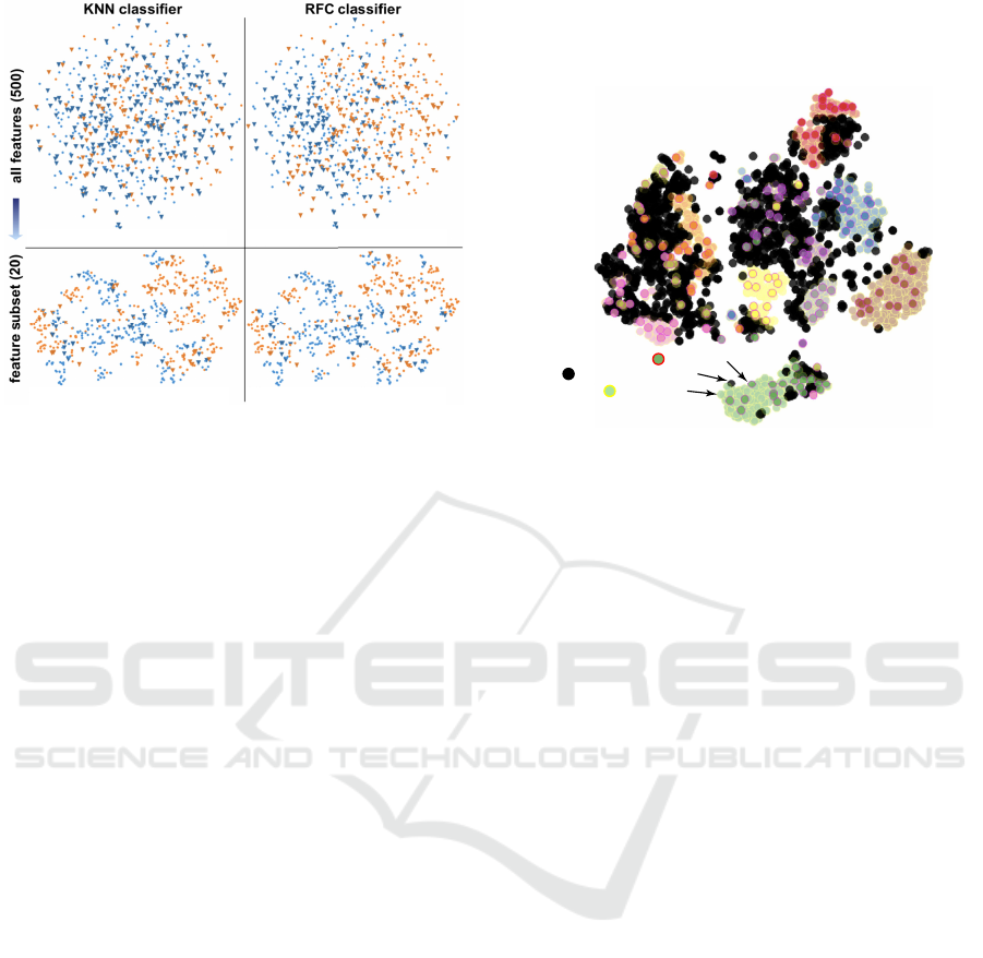
a) poor visual separation, AC=54% b) poor visual separation, AC=66%

c) good visual separation, AC=88% d) good visual separation, AC=89%

Figure 1: Classiﬁcation difﬁculty assessment via projec-

tions (Rauber et al., 2017b).

et al., 2017b) show that projections are good predic-

tors of classiﬁcation difﬁculty.

3.2 Pseudolabeling for ML Training

If projections are good predictors for classiﬁca-

tion accuracy, it means that their low-dimensional

(2D) space captures well the similarity of the high-

dimensional samples. Following this, the next step is

to actually use projections to engineer classiﬁer mod-

els. A ﬁrst attempt was shown by (Benato et al., 2018)

for the task of training a classiﬁer from a training

set having only very few labeled points: The entire

training set, including unlabeled points, is projected

and the user explores the projection to ﬁnd unlabeled

points tightly packed around labeled ones. Following

visual conﬁrmation that the packed samples are of the

same class as the surrounded label (using a tooltip

to look at the image samples), the user selects the

former and assigns them the latter’s label. The pro-

cess quickly leads to sufﬁciently large labeled sets for

training the desired model. More interestingly, auto-

mated label propagation in the embedded space using

state-of-the-art methods leads to poorer results than

user-driven labeling, which conﬁrms the added value

of the human-in-the-loop and thus the projections.

However, the best results are obtained when hu-

mans and machine cooperate rather than aim to re-

place each other. (Benato et al., 2020) adapted the

above workﬂow to (a) use an automatic label propa-

gation for the 2D projection points where the propa-

gation conﬁdence is high; and (b) expose the remain-

ing points to manual labeling (see Fig. 2). This way,

many ‘easy to label’ points are handled automatically

whereas the user’s effort is channeled towards the dif-

ﬁcult case. This strategy led to increasing model ac-

curacy and, again, surpassed conﬁdence-based label

propagation into the high-dimensional space.

supervised

auto-labeled

candidates for manual

Figure 2: Semi-automatic label propagation for construct-

ing training sets. An algorithm propagates ground-truth la-

bels from a small set of supervised samples towards neigh-

bor samples. When this algorithm is uncertain, samples are

left for manual labeling (Benato et al., 2020).

3.3 Understanding DL Models

Projections can be used not only to understand the

end-to-end behavior of classiﬁer models but also their

internals. This become especially useful when we

consider deep learned (DL) models which, with their

millions of parameters, are among the hardest arti-

facts in ML to understand. ‘Opening the black box’

of DL models is one of the most challenging, and also

most actual, goals of explainable AI (XAI) (Shwartz-

Ziv and Tishby, 2017; Azodi et al., 2020). Visualiza-

tion has been listed early on as the technique of choice

for this endeavor (Tzeng and Ma, 2005). A recent

surve (Garcia et al., 2018) outlines a wide spectrum of

visual analytics techniques and tools used for DL en-

gineering, classiﬁed in terms of supporting the tasks

of training analysis (TA), architecture understanding

(AU), and feature understanding (FU). Given the di-

versity of these tasks, the variety of the proposed vi-

sual analytocs solutions – e.g. matrix plots, icicle

plots, parallel coordinate plots, stacked barcharts, an-

notated networks, activation maps – is not surprising.

Projections occupy a particular role among these

visualizations due to their ability to compactly cap-

ture high-dimensional data – in the limit, a projec-

tion needs a single pixel to represent an n-dimensional

point, for any n value. As such, they are very suitable

instruments to depict several aspect of a DL model.

For example, in Fig. 3a, every point denotes a high-

dimensional sample, in this case a digit image from

the SVHN dataset (Rauber et al., 2017b). The points,

VISIGRAPP 2023 - 18th International Joint Conference on Computer Vision, Imaging and Computer Graphics Theory and Applications

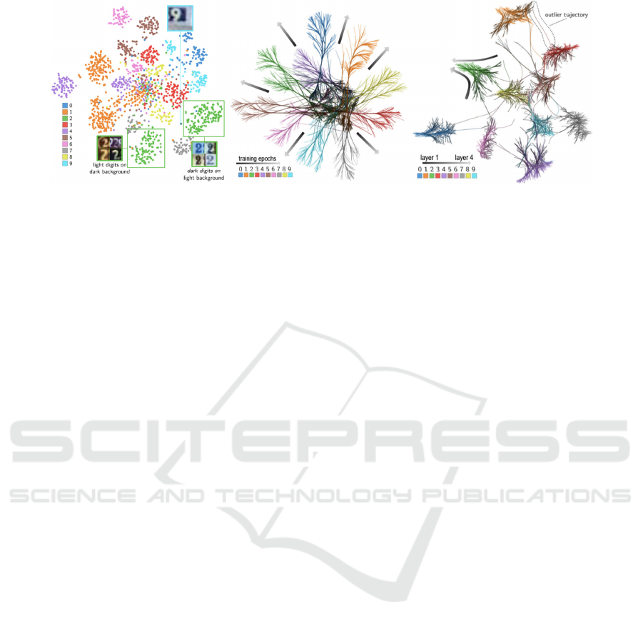
a) explore learned features b) explore training vs time c) explore training vs layers

Figure 3: Projections for understanding DL models. Exploring (a) activations of similar instances, (b) evolution of activations

over training epochs, and (c) evolution of activations over network layers (Rauber et al., 2017a).

colored by their ground-truth class, have as dimen-

sions all activations of the last hidden layer of a DL

model created to classify this dataset. We notice a

good separation of same-class images, which tells

that the model was successfully trained. We also see

two clusters of same-class points, which tell that the

model has learned to split images of the same digit

into two subclasses. Upon inspection, we see that

the model has learned by itself to separate dark-on-

bright-background digits from bright-on-dark back-

ground ones. Such ﬁndings would not be possible

without the insights given by visual tools such as pro-

jections. Moreover, such ﬁndings can help the ML

engineers to ﬁne-tune their models to increase per-

formance – in this case, eliminate the ‘color con-

trast learning’ which does not help the targeted clas-

siﬁcation. Figure 3b explores a different DL aspect,

namely how the model learns. For every epoch, a

projection of all training-set samples is made of the

samples’ last hidden layer activations, similar to im-

age (a). To maintain temporal coherence, i.e., have

similar-value samples project to close locations over

the entire set of epochs, a dynamic projection algo-

rithm, in this case dt-SNE (Rauber et al., 2016), was

used. Next, same-image points from all epochs are

connected by a trail. As the last step, trails are bun-

dled in 2D (van der Zwan et al., 2016) to reduce visual

clutter. The resulting image shows how the projection

literally fans out from a dark clump (in the middle

of the image), where last-layer neurons exhibit sim-

ilar activations for all images, to separated clusters

of same-label images. This effectively summarizes

the training success – we see, for example, that the

purple bundle (digit 4) is less well separated from

the others, which indicates some challenges in clas-

sifying this digit. Finally, Fig. 3c shows a similarly-

constructed visualization but where the trails connect

projections of test-set image activations through all

network’s hidden layers. Bundles, initially dark and

wide (layer 1), fan in, indicating that the network pro-

gressively separates images of different classes as the

data ﬂows through its layers – i.e., that the network

architecture is indeed good for the classiﬁcation task

at hand.

3.4 Decision Boundary Maps

All projections shown so far visualize a discrete set

D of samples processed by a ML model f . However,

such models are, in general, designed to accept sam-

ples from a dense set Z ⊂ R

. Classiﬁers, for instance,

partition Z into so-called decision zones (dense sets

in Z whose points get the same label) separated by

decision boundaries. Such decision boundaries are

in general complex manifolds embedded into R

and

were, until recently, only depictable for very simple

models such as logistic regression. Ideally, the ML

engineer would like to see how f behaves on the en-

tire dense space Z and not only on the sparse sampling

thereof given by training (D

) or test (D

) sets.

Since projections perform so well for visually ex-

ploring classiﬁers, it makes sense to consider extend-

ing them to depict decision zones and boundaries. In-

tuitively put, such boundaries would go through the

whitespace in a projection to separate the same-color

point clusters in e.g. Fig. 3a. Seeing decision zones

and boundaries and their relations to training and/or

test samples would help ML engineers to e.g. ﬁnd

where in the input space more training samples are

needed to improve a classiﬁer or, conversely, assess

in which such areas would samples be misclassiﬁed.

Decision boundary maps (DBMs) propose such

a visual representation for both decision zones and

boundaries for any classiﬁer. Intuitively put, DBMs

map the entire space Z (as classiﬁed by f ) to 2D rather

than the discrete sample set D, as follows. Given an

image space I ⊂ R

, a mapping P

−1

: I → R

is con-

structed to ‘backproject’ each pixel y ∈ I to a high-

Beyond the Third Dimension: How Multidimensional Projections and Machine Learning Can Help Each Other

dimensional point x = P

−1

(y). Next, y is colored by

the label f (x) assigned to it by a trained classiﬁer to

be explored. Same-color areas emerging in I indicate

f ’s decision zones; pixels on the frontiers of these ar-

eas show f ’s decision boundaries. The key to DBM

construction is creating the mapping P

−1

. One way to

do this, shown in Fig. 4a, is to use distance-based in-

terpolation over the points P(D) of a parametric (that

is, OOS) projection of the training and/or test set of

f (Schulz et al., 2015; Schulz et al., 2020). Another

way, shown in Fig. 4b, is to general purpose so-called

inverse projection techniques (Rodrigues et al., 2018).

Finally, one can construct P

−1

by using deep learning

(Fig. 4c), as discussed further in Sec. 4.2.

DBMs can be further enhanced to encode, via

brightness, the classiﬁer’s conﬁdence at every 2D

pixel (Figs. 4a,c) or actual n-dimensional distance to

the closest decision boundary (Fig. 4b). The appear-

ing brightness gradients tell which areas in the projec-

tion space are more prone to misclassiﬁcations. Im-

portantly, this does not require actual samples to exist

in a training or test set in these areas – rather, such

samples are synthesized by P

−1

4 ML FOR ASSISTING DR

Section 3 has shown several examples of the added

value of projections for ML engineering. However,

as noted in Sec. 2.3, not all projection techniques sat-

isfy all desirable requirements needed for them to be

readily used in ML visualization (and, actually, in

other contexts as well). An important question is thus:

Which projection techniques are the best candidates

for such use-cases?

A recent survey (Espadoto et al., 2019a) addressed

this question at scale for the ﬁrst time by comparing

44 projection techniques P over 19 datasets D from

the perspective of 6 quality metrics M, using grid-

search to explore the hyperparameter spaces of the

projection techniques. This is to date the only large-

scale survey that quantitatively assesses DR methods

over many datasets, techniques, quality metrics, and

parameter settings. Equally important, all its results –

datasets, projection techniques, quality metric imple-

mentations, study protocol – are automated and freely

available, much like similar endeavors in the ML

arena. Following the survey’s results, four projection

methods consistently scored high on quality for all

datasets (UMAP (McInnes et al., 2018), t-SNE (van

der Maaten and Hinton, 2008), IDMAP (Minghim

et al., 2006), and PBC (Paulovich and Minghim,

2006)), with several others close to them. However,

none of the top-ranked surveyed techniques also met

the OOS, computational scalability, and stability cri-

teria. As such, we can conclude that better DR tech-

niques are needed.

4.1 Deep Learning Projections

Following the analogy with ML regressors (Sec. 2.3,

it becomes interesting to consider ML for building

better projection algorithms. Autoencoders (Hinton

and Salakhutdinov, 2006) do precisely that and meet

all requirements in Sec. 2.3 except quality – the re-

sulting projections have in general poorer trustwor-

thiness and continuity than state-of-the-art methods

like UMAP and t-SNE. Figure 5 illustrates this: The

well-known MNIST dataset, which is well separable

into its 10 classes by many ML techniques, appears,

wrongly, poorly separated when projected by autoen-

coders. Following (Rauber et al., 2017b) (see also

Sec. 3.1, we can conclude that autoencoders are a

poor solution for DR.

Recently, Espadoto et al. (Espadoto et al., 2020)

proposed Neural Network Projections (NNP), a su-

pervised approach to learning DR: Given any dataset

D and its projection P(D) computed by the user’s

technique of choice P, a simple three-layer fully-

connected network is trained to learn to regress P(D)

when given D. Despite its simplicity, NNP can learn

to imitate any projection technique P for any dataset

D surprisingly well. While NNP’s quality is typically

slightly lower than state-of-the-art projections like t-

SNE and UMAP, it is a parametric method, stable as

proven by sensitivity analysis studies (Bredius et al.,

2022), OOS, linear in the sample count N and dimen-

sionality n (in practice, thousands of times faster than

t-SNE), and very simple to implement.

Figure 6 shows an example of the above-

mentioned sensitivity analysis. An NNP model is

trained to project the MNIST dataset, after which is

asked to project MNIST images where an increas-

ingly larger number of dimensions (pixel values) have

been cancelled, i.e., set to zero. Surprisingly, NNP

can capture the cluster structure of the data (10 classes

for the 10 digits) up to 40% cancelled dimensions.

The aggregated image shows the ‘movement’ of the

points in the NNP projection as increasingly more di-

mensions get dropped. Similar insights are obtained

for other input-dataset perturbations such as sample

jitter, translation, and scaling. At a higher level, we

see sensitivity analysis as a very powerful, yet under-

explored, technique – well known in the ML reper-

toire – to assess the quality of DR projections.

Subsequent reﬁnements included k-

NNP (Modrakowski et al., 2021) which enhances

quality by learning to project sets of neighbor sam-

VISIGRAPP 2023 - 18th International Joint Conference on Computer Vision, Imaging and Computer Graphics Theory and Applications

a c

Figure 4: Decision boundary maps for classiﬁer analysis with luminance encoding classiﬁer conﬁdence (a,c) (Schulz et al.,

2015; Rodrigues et al., 2019), respectively distance-to-decision-boundary (c) (Oliveira et al., 2022).

a) t-SNE

b) NNP c) kNNP

d) autoencoder e) SSNP

Figure 5: Projection of MNIST dataset with (a) t-SNE (van der Maaten and Hinton, 2008) and with deep learning methods:

(b) NNP (Espadoto et al., 2020), (c) kNNP (Modrakowski et al., 2021), (d) autoencoders (Hinton and Salakhutdinov, 2006),

(e) SSNP (Espadoto et al., 2021b). For supervised methods, (k)NNP succeeds in well imitating t-SNE. For self-supervised

methods, SSNP yields better quality than autoencoders.

ples; SSNP (Espadoto et al., 2021b) which works

in a self-supervised way, similar to autoencoders,

thus dispensing of the need of a training projection

and also being able to create inverse projections (see

next Sec. 4.2); SDR-NNP (Kim et al., 2022) which

increases NNP’s quality by pre-sharpening the input

training set D

via mean shift; and HyperNP (Appleby

et al., 2022), which learns the behavior of a projec-

tion technique P for all its hyperparameter values.

Figure 5 shows several of these techniques applied

to the well-known MNIST dataset which illustrates

the qualitative comments made above. All in all, the

above results prove that DL is a serious contender

for generating projections that comply with all

requirements set forth by practice.

4.2 Deep Learning Inverse Projections

Following the success of DL for constructing projec-

tions P outlined above, it becomes immediately inter-

esting to ask if we cannot do the same to construct in-

verse projections P

−1

. Introduced in Sec. 3.4 for con-

structing DBMs, inverse projections have additional

uses, e.g., generating synthetic samples for data aug-

mentation scenarios.

Espadoto et al. (Espadoto et al., 2019b) answered

the above question positively by simply ‘switching’

the input and output of NNP, i.e., given a dataset D

that projects to a 2D scatterplot by some technique

P, train a regressor to output D when given P(D).

This technique, called NNInv, inherits all the desir-

able properties of NNP (see Sec. 2.3) and also pro-

duces higher-quality DBMs than earlier models for

−1

. In particular, NNInv – and also SSNP, the other

deep-learning technique able to create inverse projec-

tions introduced in Sec. 4.1 – are about two orders of

magnitude faster than other existing inverse projec-

tion techniques such as iLAMP (Amorim et al., 2012)

and RBF (Amorim et al., 2015). NNInv was further

explored in detail for visual analytics scenarios in-

volving dynamic imputation and exploring ensemble

classiﬁers (Espadoto et al., 2021a). Figure 7 shows

the latter use-case: In the image, each pixel is back-

projected and ran through a set of nine classiﬁers,

trained to separate classes 1 and 7 from the MNIST

dataset. The pixel is then colored to indicate the clas-

siﬁers’ agreement. Deep blue, respectively red, zones

show areas where all classiﬁers agree with class 1, re-

spectively 7. Brighter areas indicate regions of high

classiﬁer disagreement – which are thus highly difﬁ-

cult to decide upon and are prime candidates for ML

engineering, regardless of the used classiﬁer.

Beyond the Third Dimension: How Multidimensional Projections and Machine Learning Can Help Each Other

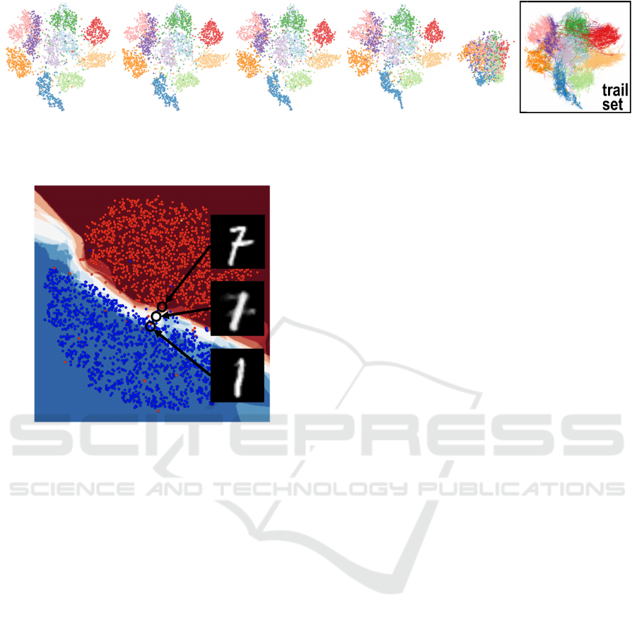
10% 20% 30% 40% 90% aggregation

Figure 6: NNP sensitivity analysis when removing between 10% and 90% of the MNIST dimensions. Surprisingly, NNP can

robustly depict the data structure even when a large part of the input information is missing (Bredius et al., 2022).

Figure 7: Classiﬁer agreement map for 9 classiﬁers, MNIST

datasets digits 1 and 7. Dark colors indicate more of the 9

classiﬁers agreeing, at a pixel in the map, with the deci-

sion (red=1, blue=7). Brighter, desaturated, colors indicate

fewer classiﬁers in agreement (white=4 classiﬁers say 1, the

other 5 say 7, or conversely) (Espadoto et al., 2021a).

5 THE WAY FORWARD

Figure 8 summarizes the tight interaction between

ML and DR described above. The central box (blue)

depicts the typical ML pipeline which maps some

input real-valued dataset D into class labels or an-

other real-valued signal by means of a classiﬁer,

respectively regressor. The box atop this pipeline

(green) shows various visualizations that cane used

to assist ML engineering, such as semi-automatic la-

beling (Sec. 3.2), assessing classiﬁcation difﬁculty

(Sec. 3.1), and assessing training and deep mod-

els (Sec. 3.3). The bottom box (yellow) uses ML

regressors to build several DR techniques such as

(self-)supervised projections (Sec. 4.1) and inverse

projections (Sec. 4.2). In turn, these lead to reﬁned

visualization methods – sensitivity analysis to assess

learned projections (Sec. 4.1) and quality analysis for

inverse projections (see Sec. 5.2 further). Finally, all

these DR methods can be used to construct the earlier-

described visualizations that assist ML engineering

(red arrow in Fig. 8).

Reﬂecting upon the current achievements of us-

ing ML for DR and conversely, we see a bright

future ahead for research where the two direc-

tions strengthen each other. A few selected, non-

exhaustive, examples of such potential ML-DR syn-

ergies are outlined next.

5.1 Prospects of DR Helping ML

Better DBMs. While current techniques allow the

fast creation of accurate DBMs (Sec. 3.4), some fun-

damental trade-offs still exist. Very accurate tech-

niques exist which solve the inherent ill-posedness

of inverting a projection function P which can map

different high-dimensional points to the same low-

dimensional location (Schulz et al., 2015; Schulz

et al., 2020). However, such techniques make various

assumptions on the underlying projections, are quite

complex to implement, and also computationally ex-

pensive – they are far from real-time adaptation of the

DBM upon re-training a classiﬁer, which would be

ideal for ML engineering (see below). Conversely,

DL-based techniques like NNInv and SSNP are near-

real-time and simple to implement but may create er-

rors that ultimately mislead their users. We foresee

possibilities of using ML, and in particular DL, to im-

prove the latter to match the quality of the former.

DBMs in Use. DBMs are not a goal in themselves,

but a tool serving a goal. Apart from the scenarios

depicted in (Espadoto et al., 2021a), DBMs could be

readily used in a visual analytics explorative scenario

to drive a classiﬁer’s training. If computable in real-

time, users could visualize the DBMs, ﬁnd problem-

atic areas with respect to how the decision boundaries

wrap around samples, and next modify the training

set by e.g. adding or deleting labels, adding new aug-

mented samples, or even moving samples. We envis-

age a tool in which users could effectively ‘sculpt’ the

shape of decision boundaries by sample manipulation

much as one edits 2D shapes by manipulating spline

control points. This would offer unprecedented free-

VISIGRAPP 2023 - 18th International Joint Conference on Computer Vision, Imaging and Computer Graphics Theory and Applications

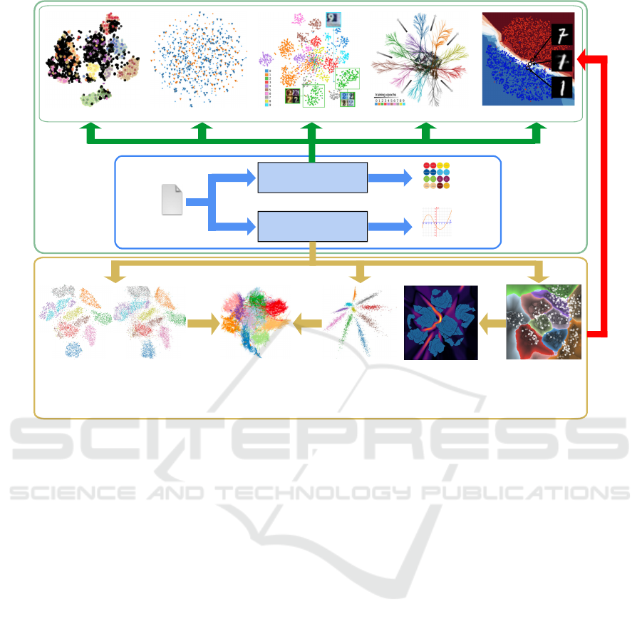
pseudolabeling classif. difficulty assessment feature understanding training assessment

classifier

regressor

input data

output labels

output signal

model assessment

supervised DR self-supervised DR inverse projectionssensitivity analysis quality analysis

Machine

learning

Dimensionality

reduction

pipeline

Figure 8: Interactions between machine learning (ML) and dimensionality reduction (DR). See Sec. 5.

dom and a wholly new way of ﬁne-tuning classiﬁers

to extend the approaches pioneered in (Benato et al.,

2018; Benato et al., 2020).

Visualizing Regressors. The examples shown in this

paper have arguably convinced the reader that pro-

jections are efﬁcient and effective in visualizing both

high-dimensional data and classiﬁer models working

on such data. However, as Sec. 2 mentions, ML is

also about a second type of technique, namely regres-

sors. A very complex, but high-potential, challenge is

to adapt and extend DR methods to visualize regres-

sors (ﬁrst of the single-variate type, then the multi-

variate one). This is fundamentally hard as the 2D vi-

sual space does not readily offer the possibility of dis-

playing many values at a single point. In some sense,

it seems that a second DR pass would be needed to re-

duce the regressor’s output dimension to what could

be displayed in 2D. Generalizing DBMs from classi-

ﬁers to ‘regressor maps’ would open a wide spectrum

of possibilities going beyond ML, e.g., in operations

research and optimization applications. A recent at-

tempt in this direction was shown in (Espadoto et al.,

2021c). However, this approach only treated single-

variate regressors f : R

→ R and used a relatively

low-quality projection (PCA).

5.2 Prospects of ML Helping DR

Learning Styles. All current DL-based projection

methods use relatively simple cost functions – ei-

ther aiming to globally mimic a training projection

(NNP-class methods) or aiming to globally minimize

some reconstruction loss (autoencoder-class meth-

ods). A ﬁrst extension direction would be to re-

ﬁne this loss to e.g. create projections where the

sizes and/or shapes of clusters can be controlled by

data attributes. One high-potential direction would be

to create a hierarchy-aware projection algorithm that

would combine the advantages of treemaps and clas-

sical projections, in the wake of earlier ideas in this

class (Duarte et al., 2014). A second extension would

be to design local cost functions that attempt to con-

struct the projection by combining different criteria

for different subsets of the input data – for example,

to achieve a globally-better projection that locally be-

haves like t-SNE in some areas and like UMAP in

others. ML techniques can help here by e.g. extend-

ing the HyperNP idea (Appleby et al., 2022) to train

from a set of projection techniques run on the same

input dataset. Further inspiration can be gotten from

recent ways in which DL is used for image synthesis

and style transfer, e.g., (Luan et al., 2017).

Beyond the Third Dimension: How Multidimensional Projections and Machine Learning Can Help Each Other

Inverse Projection Quality. Only a handful of qual-

ity metrics exist to gauge how good inverse projec-

tion techniques are (Sec. 4.2). This is not surprising

since the main use-case of such tools is to create new

data points for locations in the 2D image where no

existing data point projects. As such, deﬁning what

a good inverse projection should return in such areas

is conceptually hard. Yet, possibilities exist. One can

e.g. use a ML approach where an unseen test set is

kept apart from the construction of the inverse pro-

jection and is used to assess the quality of such a

trained model. For this, suitable distance approxima-

tions need to be designed, which can borrow from ex-

isting ML approaches to assess regressors. An equally

interesting question is how to design a scale, or hier-

archy, of errors. It is likely that differently inversely-

projected points x

′

= P

−1

(P(x)) that deviate from its

ground-truth location x by the same distance ∥x

′

− x∥

are not equally good, or equally bad, depending on

the application perspective. As such, inverse projec-

tion quality metrics may need to be designed in an

application-speciﬁc way.

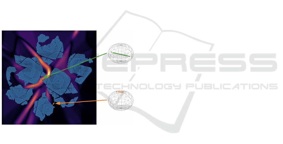
Figure 9: Gradient map of NNInv inverse projection con-

structing from a t-SNE projection of an uniformly sam-

pled sphere. Hot map regions indicate nearby 2D points

that inversely project to far-apart nD points (green line, top

sphere). Dark map regions indicate nearby 2D points that

inversely project to close nD points (orange line, bottom

sphere). The map captures thus the joint projection-inverse

projection errors (Espadoto et al., 2021a).

Figure 9 shows another challenge of measuring in-

verse projection quality. The image shows a so-called

gradient map which encodes the gradient magnitude

of the P

−1

function (in this case constructed with

NNInv). Hot regions on this map indicate nearby 2D

points which backproject far away from each other.

However, we cannot directly say that this is an er-

ror of the inverse projection P

−1

– these regions may

well correspond to areas where the direct projection

P, in this case t-SNE, squeezed faraway data points

to ﬁt them in the 2D space – thus areas of low con-

tinuity (Venna and Kaski, 2006). It is thus essential,

when designing inverse projection errors, to be able

to factor out errors induced by the direct projection.

Dynamic Projections. Section 3.3 has brieﬂy intro-

duced dynamic projections. These are extensions of

the standard, static, projection techniques which aim

to handle a dataset consisting of high-dimensional

points which maintain their identity while changing

their attribute values through time. Dynamic pro-

jections have a wealth of applications – simply put,

anywhere one wants to study high-dimensional data

which changes over time. However, only a handful

of dynamic projection techniques exist (Vernier et al.,

2021; Vernier et al., 2020), and their quality – as

gauged by established quality metrics – is good in

data structure preservation or data dynamics preser-

vation but not both aspects. Designing a dynamic

projection technique that accurately maps both data

structure and dynamics is a grand challenge for the

infovis community. Following good recent results

in using ML for DR, it looks highly interesting to

explore ML (and in particular DL) for creating dy-

namic projections. A sub-challenge here is that, since

good ground-truth dynamic projections are hard to

construct, the supervised way (NNP-class methods)

may be hard to follow, so the self-supervised direc-

tion seems more promising.

6 CONCLUSIONS

For a long time, the research topics of dimensional-

ity reduction (DR) and machine learning (ML) have

evolved in parallel and with only tangential encoun-

ters. In recent years, however, the two domains have

grown increasingly close, spurred by two develop-

ments. On the ML side, and largely due to the XAI

movement aiming at opening the ‘black box’ of ML

(and in particular deep learning) models, there is in-

creasing awareness and usage of information visual-

ization techniques to explore ML artifacts. On the DR

side, increasingly better projection methods in terms

of a wide range of quality aspects (e.g., accuracy,

speed, stability, to mention just a few) have appeared,

which are readily adopted to create new visual tools

for ML exploration. More recently, the DR commu-

nity has also started to adopt ML techniques to cre-

ate better projection algorithms. Operational difﬁcul-

ties such as poorly scalable and/or hard-to-replicate

algorithms are disappearing. As such, all is there for

cross-fertilization between ML and DR.

We see this convergence trend which unites re-

search and researchers in DR and ML growing in the

VISIGRAPP 2023 - 18th International Joint Conference on Computer Vision, Imaging and Computer Graphics Theory and Applications

near future, with both areas positively feeding each

other in terms of research questions and tasks, and

also solutions. A strong common mathematical back-

ground also unites researchers in the two ﬁelds, mak-

ing it easy to exchange research questions, ideas, and

results. We also see several high-potential research di-

rections at the crossroads of ML and DR: using dense

maps to explore and improve classiﬁers and regres-

sors, effectively mapping the whole high-dimensional

space to an image; using ML to create highly cus-

tomized, high-quality projections for both static and

dynamic data; and developing inverse projections to

meet all the standards that current direct projection

techniques have. Such developments, jointly enabled

by DR and ML researchers, will have impact far be-

yond these two ﬁelds.

REFERENCES

Amorim, E., Brazil, E., Daniels, J., Joia, P., Nonato, L.,

and Sousa, M. (2012). iLAMP: Exploring high-

dimensional spacing through backward multidimen-

sional projection. In Proc. IEEE VAST.

Amorim, E., Brazil, E., Mena-Chalco, J., Velho, L., Nonato,

L. G., Samavati, F., and Sousa, M. (2015). Facing the

high-dimensions: Inverse projection with radial basis

functions. Computers & Graphics, 48:35–47.

Appleby, G., Espadoto, M., Chen, R., Goree, S., Telea, A.,

Anderson, E., and Chang, R. (2022). HyperNP: Inter-

active visual exploration of multidimensional projec-

tion hyperparameters. CGF, 41(3):169–181.

Azodi, C., Tang, J., and Shiu, S. (2020). Opening the black

box: Interpretable machine learning for geneticists.

Trends Genet, 36(6):442–455.

Benato, B., Gomes, J., Telea, A., and Falc

ao, A. (2020).

Semi-automatic data annotation guided by feature

space projection. Pattern Recognition, 109:107612.

Benato, B., Telea, A., and Falc

ao, A. (2018). Semi-

supervised learning with interactive label propagation

guided by feature space projections. In Proc. SIB-

GRAPI, pages 392–399.

Botchkarev, A. (2019). Performance metrics (error mea-

sures) in machine learning regression, forecasting and

prognostics: Properties and typology. Interdisci-

plinary J. of Information, Knowledge, and Manage-

ment, 14:45–79.

Bredius, C., Tian, Z., and Telea, A. (2022). Visual explo-

ration of neural network projection stability. In Proc.

MLVis.

Duarte, F., Sikanski, F., Fatore, F., Fadel, S., and

Paulovich, F. V. (2014). Nmap: A novel neighborhood

preservation space-ﬁlling algorithm. IEEE TVCG,

20(12):2063–2071.

Espadoto, M., Appleby, G., A. Suh, D. C., Li, M.,

Scheidegger, C., Anderson, E., Chang, R.,

and Telea, A. (2021a). UnProjection: Lever-

aging inverse-projections for visual analyt-

ics of high-dimensional data. IEEE TVCG.

DOI:10.1109/TVCG.2021.3125576.

Espadoto, M., Hirata, N., and Telea, A. (2020). Deep learn-

ing multidimensional projections. Information Visual-

ization, 9(3):247–269.

Espadoto, M., Hirata, N., and Telea, A. (2021b). Self-

supervised dimensionality reduction with neural net-

works and pseudo-labeling. In Proc. IVAPP.

Espadoto, M., Martins, R., Kerren, A., Hirata, N., and

Telea, A. (2019a). Toward a quantitative survey

of dimension reduction techniques. IEEE TVCG,

27(3):2153–2173.

Espadoto, M., Rodrigues, F. C. M., Hirata, N., and Telea,

A. (2021c). OptMap: Using dense maps for visualiz-

ing multidimensional optimization problems. In Proc.

IVAPP.

Espadoto, M., Rodrigues, F. C. M., Hirata, N. S. T., Jr,

R. H., and Telea, A. (2019b). Deep learning inverse

multidimensional projections. In Proc. EuroVA.

Garcia, R., Telea, A., da Silva, B., Torresen, J., and Comba,

J. (2018). A task-and-technique centered survey on

visual analytics for deep learning model engineering.

Computers and Graphics, 77:30–49.

Geurts, P., Ernst, D., and Wehenkel, L. (2006). Extremely

randomized trees. Machine learning, 63(1):3–42.

Guyon, I., S, S. G., and Ben-Hur, A. (2004). Result anal-

ysis of the NIPS 2003 feature selection challenge. In

Advances in Neural Information Processing Systems,

page 545?552.

Hinton, G. E. and Salakhutdinov, R. R. (2006). Reducing

the dimensionality of data with neural networks. Sci-

ence, 313(5786):504–507.

Jiang, T., Gradus, J., and Rosellini, A. (2020). Supervised

machine learning: A brief primer. Behavior Therapy,

51(5):675–687.

Kim, Y., Espadoto, M., Trager, S., Roerdink, J., and Telea,

A. (2022). SDR-NNP: Sharpened dimensionality re-

duction with neural networks. In Proc. IVAPP.

Lespinats, S. and Aupetit, M. (2011). CheckViz: Sanity

check and topological clues for linear and nonlinear

mappings. CGF, 30(1):113–125.

Luan, F., Paris, S., Shechtman, E., and Bala, K. (2017).

Deep photo style transfer. In Proc. IEEE CVPR.

McInnes, L., Healy, J., and Melville, J. (2018). UMAP:

Uniform manifold approximation and projection for

dimension reduction. arXiv:1802.03426v2 [stat.ML].

Minghim, R., Paulovich, F. V., and Lopes, A. A. (2006).

Content-based text mapping using multi-dimensional

projections for exploration of document collections.

In Proc. SPIE. Intl. Society for Optics and Photonics.

Modrakowski, T., Espadoto, M., Falcao, A., Hirata, N., and

Telea, A. (2021). Improving deep learning projections

by neighborhood analysis. In Communication in Com-

puter and Information. Springer.

Nonato, L. and Aupetit, M. (2018). Multidimensional

projection for visual analytics: Linking techniques

with distortions, tasks, and layout enrichment. IEEE

TVCG.

Beyond the Third Dimension: How Multidimensional Projections and Machine Learning Can Help Each Other

Oliveira, A. A. M., Espadoto, M., Hirata, R., and Telea, A.

(2022). SDBM: Supervised decision boundary maps

for machine learning classiﬁers. In Proc. IVAPP.

Paulovich, F. V. and Minghim, R. (2006). Text map ex-

plorer: a tool to create and explore document maps.

In Proc. IEEE IV, pages 245–251.

Rauber, P., Fadel, S. G., Falc

ao, A., and Telea, A. (2017a).

Visualizing the hidden activity of artiﬁcial neural net-

works. IEEE TVCG, 23(1):101–110.

Rauber, P., Falcao, A., and Telea, A. (2016). Visualizing

time-dependent data using dynamic t-SNE. In Proc.

EuroVis – short papers, pages 43–49.

Rauber, P. E., Falc

ao, A. X., and Telea, A. C. (2017b). Pro-

jections as visual aids for classiﬁcation system design.

Inf Vis, 17(4):282–305.

Rodrigues, F. C. M., Espadoto, M., Jr, R. H., and Telea,

A. (2019). Constructing and visualizing high-quality

classiﬁer decision boundary maps. Information,

10(9):280–297.

Rodrigues, F. C. M., Jr., R. H., and Telea, A. (2018). Image-

based visualization of classiﬁer decision boundaries.

In Proc. SIBGRAPI.

Schulz, A., Gisbrecht, A., and Hammer, B. (2015). Us-

ing discriminative dimensionality reduction to visual-

ize classiﬁers. Neural Process. Lett., 42(1):27–54.

Schulz, A., Hinder, F., and Hammer, B. (2020). DeepView:

Visualizing classiﬁcation boundaries of deep neural

networks as scatter plots using discriminative dimen-

sionality reduction. In Bessiere, C., editor, Proc. IJ-

CAI, pages 2305–2311.

Shwartz-Ziv, R. and Tishby, N. (2017). Opening the

black box of deep neural networks via information.

arXiv:1703.00810 [cs.LG].

Thiyagalingam, J., Shankar, M., Fox, G., and Hey, T.

(2022). Scientiﬁc machine learning benchmarks. Na-

ture Reviews Physics, 4:413–420.

Tzeng, F. Y. and Ma, K.-L. (2005). Opening the black box –

data driven visualization of neural networks. In Proc.

IEEE Visualization.

van der Maaten, L. and Hinton, G. E. (2008). Visualizing

data using t-sne. JMLR, 9:2579–2605.

van der Zwan, M., Codreanu, V., and Telea, A. (2016).

CUBu: Universal real-time bundling for large graphs.

IEEE TVCG, 22(12):2550–2563.

Venna, J. and Kaski, S. (2006). Visualizing gene interaction

graphs with local multidimensional scaling. In Proc.

ESANN, pages 557–562.

Vernier, E., Comba, J., and Telea, A. (2021). Guided sta-

ble dynamic projections. Computer Graphics Forum,

40(3):87–98.

Vernier, E., Garcia, R., da Silva, I., Comba, J., and Telea,

A. (2020). Quantitative evaluation of time-dependent

multidimensional projection techniques. Computer

Graphics Forum, 39(3):241–252.

VISIGRAPP 2023 - 18th International Joint Conference on Computer Vision, Imaging and Computer Graphics Theory and Applications